Modeled Land Atmosphere Coupling Response to Soil Moisture Changes with Different Generations of Land Surface Models

Abstract

An idealized study with two land surface models (LSMs): TERRA-Multi Layer (TERRA-ML) and Community Land Model (CLM) alternatively coupled to the same atmospheric model COSMO (Consortium for Small-Scale Modeling), reveals differences in the response of the LSMs to initial soil moisture. The bulk parameterization of evapotranspiration pathways, which depends on the integrated soil moisture of active layers rather than on each discrete layer, results in a weaker response of the surface energy flux partitioning to changes in soil moisture for TERRA-ML, as compared to CLM. The difference in the resulting surface energy flux partitioning also significantly affects the model response in terms of the state of the atmospheric boundary layer. For vegetated land surfaces, both models behave quite differently for drier regimes. However, deeper reaching root fractions in CLM align both model responses with each other. In general, differences in the parameterization of the available root zone soil moisture, evapotranspiration pathways, and the soil-vegetation structure in the two LSMs are mainly responsible for the diverging tendencies of the simulated land atmosphere coupling responses.

1. Introduction

Many numerical weather prediction (NWP) models still rely on the relatively simple representation of the terrestrial ecosystem with second generation land surface models (LSMs), which do not simulate carbon fluxes. Substantial effort has been made to investigate the importance of a better representation of the biogeophysical and biogeochemical processes in LSMs in the context of weather and climate simulations (e.g., [1,2,3,4,5,6,7,8]). The inclusion of a land surface model with a more process-based representation of vegetation including the lateral flow of soil moisture led to improvements in the predicted local weather over Western Germany [1]. Their model simulation showed better agreements to measured surface energy fluxes, atmospheric boundary layer (ABL) structure, and precipitation. Similarly, the use of a third generation LSM (Community Land Model; CLM) led to improvements in the simulated summertime surface air temperature over the western U.S.A., as compared to observations [2]. In addition, the inclusion of CLM led to substantial improvements in summertime radiation fluxes (via the improvement in cloud cover) and partitioning of turbulent fluxes with climate simulation over Europe [3]. The superiority of CLM (among multiple LSMs), particularly in simulating the surface temperature maximum for regional climate simulations over U.S.A was also presented by [4]. However, they could not find any significant sensitivity of the spatial and temporal variability of precipitation to different LSMs. In another effort, a multiple combination of LSMs and ABL schemes was used to diagnose the land-atmosphere coupling over the southern great plains (SGP) for dry (<25% volumetric soil moisture) and wet (near saturation) extremes using diurnal scale simulations [5]. They found that CLM generally simulated the evaporative fluxes in wet regimes better, which, however did not translate into better coupling metrics, as the land surface influence is diminished relative to the ABL during wet regimes. In the continuing effort to add more physically based processes, the inclusion of CLM and a 3-D groundwater model led to slight improvements in the simulated diurnal surface fluxes over Western Germany [6]. Further, the inclusion of CLM with a 3-D groundwater model in a regional simulation over Europe attenuated the land-atmosphere coupling for the simulated heat wave of 2003 via controls on the root zone soil moisture [7]. This was also found to have stronger dependence on the uncertainty in representation of sub-surface heterogeneity. In another study, the skills of two different generations of LSMs (coupled to the same atmospheric model) were evaluated using convection-permitting seasonal scale simulations over Western Germany. Although, both configurations systematically underestimated the seasonal average diurnal cycle of evapotranspiration for five stations, the third generation LSM (CLM) with the inclusion of a 3D-groundwater model had a lower bias. However, this study also could not identify any clear change in the spatial and temporal variation of precipitation like the earlier study [4].

The studies above demonstrate the importance of sophisticated LSMs in the simulated land atmosphere interactions, although uncertainty persists about their feedbacks on cloud and precipitation. However, the nature and strength of the land-atmospheric coupling resulting from different LSMs also appears to vary significantly between wet and dry regimes with stronger coupling for the latter. Additionally, the changes in the model response when using different LSMs coupled with the atmospheric model in real-world data settings, becomes less tractable due to the complexity in the spatial patterns of soil-vegetation-atmosphere states and the resulting two-way interactions. Recently, a second (TERRA-Multi Layer (TERRA-ML), [9,10,11,12]) and a third-generation land surface model (Community Land Model (CLM) version 3.5, [13]) were evaluated with multi-year observation driven simulations at the Falkenberg grassland site in Germany. The study showed that both models tend to overestimate the Bowen ratio, while CLM exhibited a wet bias. With modified photosynthetic parameters, CLM was found to be superior in accurately simulating the Bowen ratio, but it did not improve the soil moisture variance adequately (especially during periods of recession, where the upper shallow root zone layer enters a dry regime). However, the simulated Bowen ratio became worse, when correcting the vertical profile of soil moisture using data assimilation (resulting in lower available root zone soil moisture). This also led to the identification of the simplified assumption of the default shallow root fraction distribution, which remains invariant during the simulation. Using a deeper root fraction distribution, CLM was able to simulate better flux partitioning and soil states as compared to TERRA-ML. In general, the effect of the root fraction distribution is masked during wet regimes. However, for shallow dry regimes (≤30 cm) in periods of recession, the specification of vertical profile of the root fraction distribution is a source of uncertainty in the pathways of evapotranspiration. Especially for coupled weather and climate simulations, rainfall and recession periods are omnipresent (representing transitions from wet to dry regimes) at different temporal and spatial scales. Consequently, the spatial patterns of surface fluxes will also vary depending on available root zone soil moisture, which is co-dependent on the vertical profile of the root distribution and soil moisture. Since the ABL responds to the surface energy, moisture, and momentum fluxes from the land surface, it is thus imperative to better understand the mechanisms which govern the exchange fluxes especially during transitions from dry to wet regimes (or vice-versa).

In this study, we explore the nature and strength of land atmosphere coupling in such transitions based on idealized settings for both, TERRA-ML and CLM coupled to the same atmospheric model COSMO (Consortium for Small-Scale Modeling, [14]) using the Terrestrial Systems Modeling Platform (TerrSysMP, [6]). This study makes an effort to elucidate how and why the model response changes when using different generations of LSMs coupled to the same atmospheric model in an idealized setting. Thus, we contribute to a better understanding of the multiple processes that produce different land-atmosphere interactions when using these LSMs for weather and climate predictions with real data simulations.

A brief discussion about TerrSysMP and the models used in this study is provided in Section 2. The experiment setup and results are presented in Section 3 and Section 4 respectively, followed by discussion in Section 5. Finally, conclusions are presented in Section 6.

2. Model Description

2.1. The Modular Platform TerrSysMP

TerrSysMP [6] is a modular regional terrestrial system simulation platform consisting of different models for the atmosphere, land surface, and subsurface, coupled using the external coupler OASIS3 [15] or OASIS3-MCT [16] for an efficient use on supercomputers [17]. The platform is modular and users can choose between different model configurations. For example, a stand-alone system with any one of the individual models (COSMO, CLM, or ParFlow), a coupled hydrological modeling system (CLM and ParFlow, [18]), a fully coupled system (COSMO, CLM, and ParFlow), and a coupled land-atmosphere system without a 3D-distributed groundwater model (COSMO and CLM, [19]). In this study, we compare the results obtained with the COSMO-CLM configuration (details of the coupling between COSMO and CLM is presented in Appendix A) with results obtained using COSMO stand-alone equipped with its in-built 2nd generation land surface model TERRA-ML. In the following sections, we briefly describe the atmospheric model COSMO and the two LSMs. A more detailed discussion of the differences between the two LSMs is also available in [9].

2.2. The COSMO Weather Prediction Model

The numerical weather prediction model COSMO [14,20] is developed and maintained by an association of several European national weather services (http://www.cosmo-model.org/) led by the German national weather service DWD (Deutscher Wetterdienst). Here, we only describe the COSMO’s physics packages [21] that are important in the context of this study. A detailed description of the dynamical and physical packages available in COSMO can be found in [14]. The radiation scheme is based on the one-dimensional $\delta$-two-stream-approximation [22]. The default ABL scheme is based on a level-2.5 turbulence parameterization of [23] and a Blackadar mixing-length parameterization [24] resulting in a flux-gradient representation for sub-grid scale fluxes with diffusion coefficients and a turbulent length scale. The ABL scheme is coupled to a surface transfer scheme to compute the transfer coefficients for heat and momentum developed by [25].

2.3. TERRA-ML

TERRA-ML is the default LSM for COSMO. In the coupled mode with COSMO, TERRA-ML simulates the energy and water balance at the land surface and in the shallow subsurface, and provides the soil temperature and moisture as a lower boundary condition to the atmospheric model. All processes in TERRA-ML are modeled only in the vertical direction with no lateral interactions between adjacent soil columns.

Grid cell heterogeneity is specified by the vegetation fraction (or plant cover fraction). An explicit canopy layer is absent, and plant phenology is prescribed using minimum and maximum LAI (Leaf Area Index), a fixed roughness height and root layer depth. The homogeneous soil column is discretized into eight vertically stretched layers with lower boundaries at 0.01, 0.03, 0.09, 0.27, 0.81, 2.43, 7.29, and 21.87 m. A lookup table with 10 possible soil types provides the hydrological and thermal properties of the soil column, including the dry and wet albedo.

Vegetation temperature is assumed to be equal to the near-surface soil temperature. The soil temperature is computed using the heat conduction equation with ground heat flux and climatological annual mean surface temperature as upper and lower boundary condition. Soil water content is computed using Richard’s equation with infiltration and gravitational drainage as upper and lower boundary condition.

Surface radiation fluxes depend on ground albedo and temperature. Surface energy and momentum fluxes are computed using the surface transfer scheme [25]. Bare soil evaporation and canopy transpiration are based on the BATS scheme [26]. Bare soil evaporation is dependent on the soil moisture content of an active layer of 0.81 m depth [21]. The Jarvis-Stewart approach [27,28] is used for canopy transpiration in the stomatal conductance model. Root water uptake depends on the total transpiration rate, the root zone integrated liquid water content, and the root depth.

2.4. CLM

In CLM [13], all processes are modeled only in the vertical direction (like in TERRA-ML) with no interactions between adjacent soil columns. CLM directly simulates carbon, water and energy balance, along with the vegetation and soil states. In coupled simulations, the atmospheric forcing is obtained from the lowest level of the atmospheric model.

Grid cell heterogeneity can be represented using a subgrid tile approach with five land units, multiple soil columns, and 17 plant functional types (PFTs). We only use one PFT, one soil column, and one land unit for each CLM grid cell in this study. CLM has an explicit canopy layer with plant phenology prescribed using monthly LAI, SAI (Stem Area Index), plant top and bottom height, and fixed root distribution parameters. For the different PFTs, a lookup table provides the necessary photosynthesis, optical and, aerodynamical parameters. The vertical soil column can be heterogeneous with 10 vertically stretched layers with lower boundaries at 0.017, 0.045, 0.09, 0.16, 0.29, 0.49, 0.82, 1.38, 2.29 and 3.43 m. The hydrological and thermal property of the soil is specified using pedotransfer functions based on the specified sand and clay percentage as input.

Vegetation temperature is computed assuming that the canopy has a negligible capacity to store heat. Soil temperature is computed using the heat conduction equation with ground heat flux and zero heat flux as top and bottom boundary conditions, respectively. Soil moisture is computed using Richards equation with infiltration after interception and exchange with the unconfined aquifer as the top and bottom boundary condition respectively.

For vegetation, the two-stream approximation is used to compute surface radiation fluxes. Surface energy and momentum fluxes are computed using the Monin-Obukhov Similarity Theory, as the sum of vegetation and ground fluxes (below vegetation). For bare soil evaporation, an additional soil resistance term based on works of [29] is added to reduce excessive soil evaporation. The bare soil evaporation is dependent on the soil moisture content of the surface soil layer only. A coupled stomatal conductance and photosynthesis model [30] is used to compute canopy transpiration and carbon fluxes. For canopy transpiration, the corresponding root water uptake is estimated as a function of total transpiration, static root distribution, plant wilting factor, and a soil moisture limiting function. The limiting function is computed as an integral of plant wilting factor and fractions of roots in each active root zone layer.

3. Experiment Setup

Multiple experiments are designed to investigate the nature and strength of land-atmosphere coupling by evaluating changes in model response for two different land use types—bare soil and vegetated—with different initial soil moisture content. The initialized relative soil moisture content $(S_w)$ represents transitions of soil states from very dry ($S_w~0.2$) to wet regimes ($S_w~0.6$). Additional experiments are designed to illustrate the impact of relatively shallow dry regimes $\left(S_{w,z\le 30\mathrm{cm}}<0.5\right)$, typically observed during recession periods (e.g., [9]) on the model response, including the sensitivity to the vertical profile of the root distribution in CLM, as discussed above.

3.1. Idealized Simulations

In total, 45 diurnal evolutions of a cloud-free convective boundary layer are simulated over an area of 20 × 20 km² with 1 km grid resolution both for the atmospheric and land surface models. The simulations are conducted with TerrSysMP both in its COSMO stand-alone mode (COSMO coupled to TERRA-ML) hereafter referred to as COSMO only, and in its coupled mode with CLM, hereafter referred to as TSMP. The experiments are categorized into three groups based on soil moisture initialization and root distributions (

Table 1. Experiment Setup for COSMO (Consortium for Small-Scale Modeling) and TSMP (Terrestrial Systems Modeling Platform).

CSDR (Vertically Constant Relative Soil Saturation and Default Root Distribution)

Land Use Types: Bare Soil and Vegetated Five Soil Moisture Initialization: Vertically constant profiles $S_w=0.2, 0.3, 0.4, 0.5 and 0.6$

VSDR (Vertically Varying Relative Soil Saturation and Default Root Distribution)

Land Use Types: Bare Soil and Vegetated Soil Moisture Initialization: Vertically varying profiles $S_{w,z<30 \mathrm{c}\mathrm{m}}=0.2, 0.3, 0.4, 0.5 and 0.6$, $S_{w,z\ge 30 \mathrm{c}\mathrm{m}}=0.6$

VSMR (Vertically Varying Relative Soil SATURATION and Modified Root Distribution)

Two Land Use Types: Bare Soil, Vegetated with modified root distribution for TSMP Five Soil Moisture Initialization: Vertically varying profiles $S_{w,z<30 \mathrm{c}\mathrm{m}}=0.2, 0.3, 0.4, 0.5 and 0.6$, $S_{w,z\ge 30 \mathrm{c}\mathrm{m}}=0.6$

). For the VSMR experiment, only the root distribution in TSMP is changed; thus, VSMR and VSDR are identical for the COSMO simulations, which also apply for the TSMP bare-soil experiments.

The atmospheric domain uses the default COSMO vertically stretched grid with 50 levels and a near-surface vertical resolution of 20 m. The LSMs also use their default vertically stretched grids as explained above. All simulations start at midnight and run for 24 h. Periodic lateral boundary conditions are used for the atmospheric model with the radiation field updated every 15 min. The model and coupling time steps are set to 10 s.

3.2. Soil-Vegetation Structure

Two land use types—bare soil (bs) and vegetated (vg)—are used for the study. Land use is prescribed to be horizontally homogeneous. In TERRA-ML, these land use types are realized by using a plant cover fraction of 0.20 for bare soil and 0.90 for vegetated land (closer to maximum plant cover fraction for non-vegetated and vegetated area used in real data simulation). In CLM, the plant functional types (PFTs) crop and bare-soil were selected for vegetated and bare soil, respectively. In both TERRA-ML and CLM, the roughness height for momentum was set to 0.01 m and 0.108 m for bare soil and vegetated land use types, respectively. For vegetation, the LAI was set to 3.5 in both LSMs. The root depth was set to the default 0.6 m for TERRA-ML. For CLM, the default and a modified [9] root distribution was used. The default vertical profile of root distribution contains 80% of the root fraction within the top 50 cm of the soil depth, while the modified root distribution contains 85% of the root fractions within the top 150 cm of the soil. The soil was set horizontally homogeneous to clay-loam in TERRA-ML. For CLM, soil texture was specified by 35% sand and 34% clay, which is consistent with the default sand and clay percentage specified in TERRA-ML for clay-loam. The required input data for the CLM was generated using the TerrSysMP Pre-processing and Post-processing System (TPS, [31]).

3.3. Initial Conditions

The initial atmospheric conditions for temperature, humidity and pressure were taken from sounding data obtained over Stuttgart (Germany) under stable conditions and a vertically constant background wind speed of 1 m/s. Soil temperature and soil moisture for all levels were initialized horizontally homogeneous with temperature at 287 K and soil moisture at constant relative saturation $\left(S_w\right)$ values of 0.2, 0.3, 0.4, 0.5 and 0.6, respectively, in the layers down to 30 cm. For depths below 30 cm, $S_w$ was kept at the same value as the upper layers for the vertically constant relative soil saturation and default root distribution (CSDR) experiments, while a constant (high) value of 0.6 was used for the vertically varying relative soil saturation experiments with default and modified root distributions (VSDR and VSMR).

4. Results

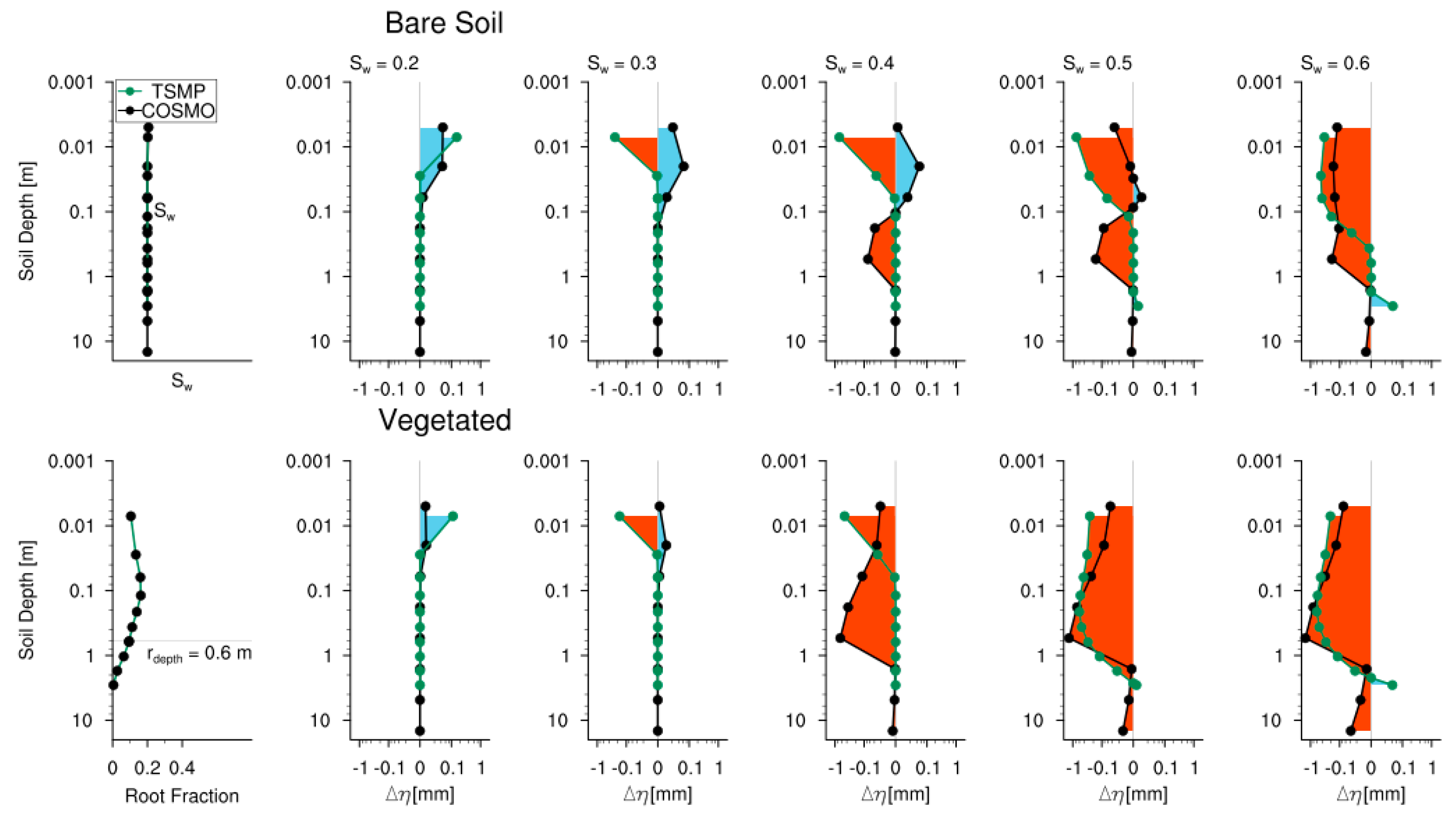
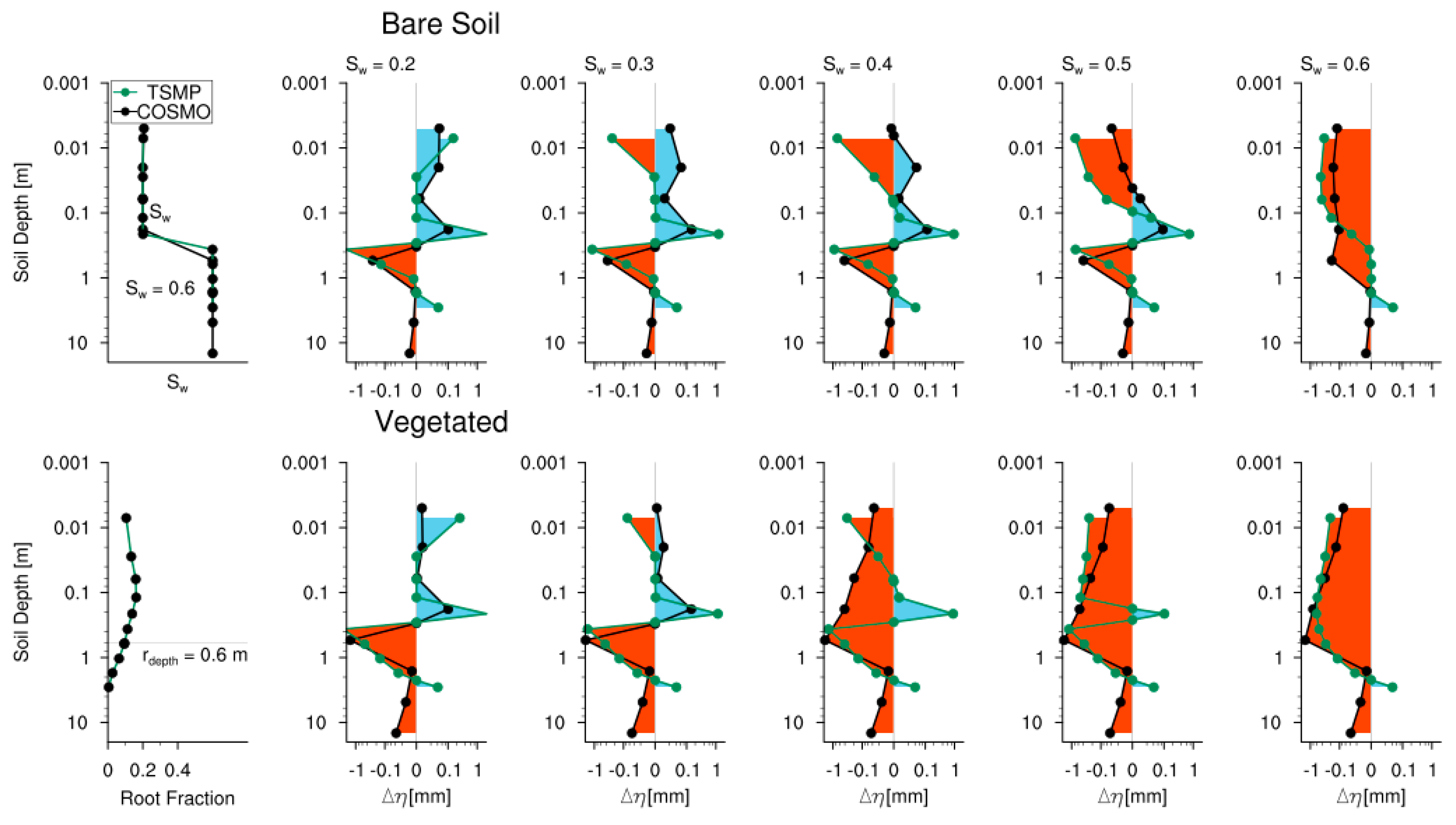
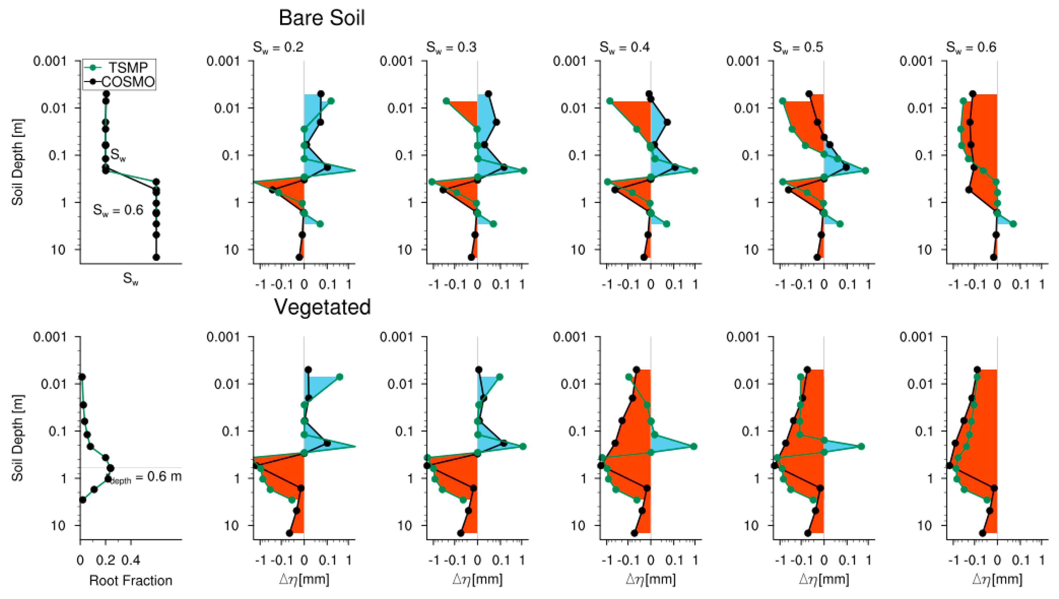
4.1. Soil Moisture Response to Initial Soil Moisture

Figure 1 shows the diurnal scale change in vertical soil moisture content $\left(\Delta \eta \right)$ for the CSDR experiments (initialized with vertically constant relative saturation and with default root distributions). $\Delta \eta$ for each soil layer is computed as

$$\Delta {\eta }_i=\left(S_{w,i}^{t=24}-S_{w,i}^{t=0}\right)\times \varnothing \times d{z}_i$$

where the terms $S_{w,i}^{t=0}$ and $S_{w,i}^{t=24}$ are the relative saturation in the beginning and end of the one-day simulation, respectively, $\varnothing$ is the porosity, and $d{z}_i$ is the soil depth of the ith layer. The initial relative saturation for the shallow upper layer $S_{w,z\le 30 \mathrm{cm}}^{t=0}$ is hereafter simply referred to as $S_w$. A modulus transformation $\left[L\left(x\right)=sign\left(x\right)\times \log (\log \left|x\right|+1)\right]$ as suggested by [32] is used to visualize the vertical profile of $\Delta \eta$, which varies by 2 to 3 orders of magnitude in both positive and negative direction. The vertically integrated diurnal change in soil moisture content $\left({\sum }_z\Delta \eta \right)$ is summarized in

Table 2. Total change in $\Delta \eta$ for the entire soil column for different initial relative soil saturation initializations (S_w).

${\mathit{S}}_{\mathit{w}}[-]$	0.2		0.3		0.4		0.5		0.6
${\sum }_z\Delta \eta \left[{m}{m}\right]$	bs	vg	bs	vg	bs	vg	bs	vg	bs	vg
CSDR Experiment
COSMO	+0.09	+0.01	+0.09	+ 0.01	−0.04	−1.19	−0.28	−2.43	−0.74	−2.87
TSMP	+0.15	+0.11	−0.25	−0.17	−0.75	−0.50	−1.10	−3.11	−1.38	−3.10
VSDR Experiment
COSMO	−0.08	−1.45	−0.13	−1.85	−0.26	−2.59	−0.36	−2.75	−0.74	−2.87
TSMP	+0.19	−0.83	−0.22	−1.12	−0.72	−1.39	−1.06	−3.11	−1.38	−3.10
VSMR Experiment
COSMO	−0.08	−1.45	−0.13	−1.85	−0.26	−2.59	−0.36	−2.75	−0.74	−2.87
TSMP	+0.19	−2.23	−0.22	−2.88	−0.72	−3.00	−1.06	−3.14	−1.38	−3.09

.

In the bare soil runs, both models generate dew during the night, which partly explains the positive $\Delta \eta$ in the upper layers for the dry soil moisture initialization ($S_w=0.2$); almost no soil evaporation takes place in these runs. At intermediate initial soil moisture values ($S_w=0.3~0.4$), the upper soil layer evaporates ($\Delta \eta$ is negative) in the TSMP run, while no significant change of soil moisture is discernable in COSMO. Soil evaporation increases for higher initial relative soil saturation at a faster rate in TSMP than in COSMO, leading to larger drops in $\Delta \eta$ in the upper shallow layer (whose depth also increases) in TSMP. At an initial soil saturation $S_w=0.4$, $\Delta \eta$ exhibits a vertical dipole behavior in the COSMO run with soil moisture increase in the upper layer (dew formation) and decrease in deeper layers (evaporation sink from active deep layer). This dipole behavior disappears for $S_w>0.4$ due to increase in soil evaporation. For $S_w=0.6$, the vertical profiles of $\Delta \eta$ tends to converge for both models, while the amplitude is smaller and the depth larger for COSMO as compared to TSMP.

For the vegetated land surface, the dew formation overnight is lower for both models as compared to the bare soil runs, which is now lower in the COSMO runs (see different, but positive $\Delta \eta$ for $S_w=0.2$ in the upper layers). For $S_w=0.3$, $\Delta \eta$ remains positive for COSMO but becomes negative for TSMP in the upper layers, with lower amplitudes as compared to the bare soil case (Table 2). At initial soil saturation $S_w=0.4$, only the shallow uppermost layer gets drier in the TSMP run while in the COSMO run almost the whole soil column significantly dries. This is consistent with its higher evapotranspiration (Table 2). For initial soil saturation $S_w\ge 0.5$, both models show very similar and overall high decreases in soil moisture. For both, bare soil and vegetated land, at $S_w\ge 0.5$, soil moisture in the TSMP run slightly increases (<0.1 mm) in the lowest level, which probably results from flux exchanges with the simplified groundwater model used in CLM as the bottom boundary condition

Figure 2 and Figure 3 show the vertical soil saturation profile changes for the VSDR (initialization with vertically varying relative soil saturation and default root distribution) and VSMR (initialization with vertically varying relative soil saturation and a modified root distribution) simulations. In both experiments, the soil moisture adjustment resulting from the sharp vertical gradient soil moisture initialization leads to the expected increase/decrease in soil moisture around 30 cm depth. This adjustment effect attenuates with increasing shallow root zone soil moisture due to the weakening of the vertical soil moisture gradient. For bare soil, higher soil saturation below 30 cm depth or the change in the root distribution (only TSMP) does not significantly impact the vertical profile of $\Delta \eta$ in the upper layers for both models. In the COSMO bare soil simulations, $\sum _z\Delta \eta$ decreases only for $S_w\ge 0.4$ (Table 2) in the CSDR experiments. However, a decrease in $\sum _z\Delta \eta$ can be observed for the VSDR and VSMR experiments independent of the initial soil moisture. This tendency results from the higher soil evaporation with increasing soil saturation in the deeper soil layers. There is no significant change in $\sum _z\Delta \eta$ for TSMP for both the VSDR and VSMR experiments as compared to the CSDR experiment (Table 2); thus, the dipole behavior caused by soil moisture adjustments barely impacts soil evaporation in TSMP.

For the vegetated land surface, the higher initial deeper-layer soil moisture clearly impacts the experiments with the vertically variable initial soil saturation (VSDR) and the additionally modified vertical root distribution (VSMR). As compared to CSDR, $\sum _z\Delta \eta$ for TSMP ($S_w=0.2$) and COSMO ($S_w=0.2, 0.3$) is negative (Table 2), indicating a net loss of soil water by evapotranspiration. The VSDR experiments result in an overall soil moisture decrease in COSMO and TSMP as compared to CSDR, especially for $S_w<0.5$. In CSDR and VSDR experiments, all COSMO simulations loose more water at $S_w\le 0.4$ as compared to the TSMP simulations. In the VSMR experiment, however, the overall soil moisture decrease enhances for TSMP with the $\Delta \eta$ peak shifting downwards (i.e., increase in available root zone soil moisture from deeper layers).

These results indicate that the soil moisture decrease due to bare soil evaporation and canopy transpiration differ between the two LSMs, especially for the drier regimes ($S_w<0.5$), which will also affect the flux and ABL evolutions which is discussed in the following sections.

4.2. Overall Model State Response to Initial Soil Moisture

In this section, we focus on the response of surface energy flux partitioning and related ABL states to variations in the initial soil moisture of the shallow upper layer (≤30 cm) in the different model setups. Changes in the model response are quantified relative to the runs with the lowest initial soil saturation $\left(S_w=0.2\right)$. To do so, we compare the mean surface fluxes between 1100 to 1400 LT over a grid point near the domain center (results would not differ much between grid columns because of homogeneous land surface and periodic boundary conditions). Similarly, ABL quantities averaged between 1300 and 1600 LT over the same grid point are compared. A later time period is chosen for ABL quantities compared to surface fluxes in order to include the period with the largest ABL height. The mean ABL virtual potential temperature$\left({\theta }_{v400 \mathrm{m}}\right)$ is computed at 400 m a.g.l., which well represents the well-mixed virtual potential temperature of the whole profile.

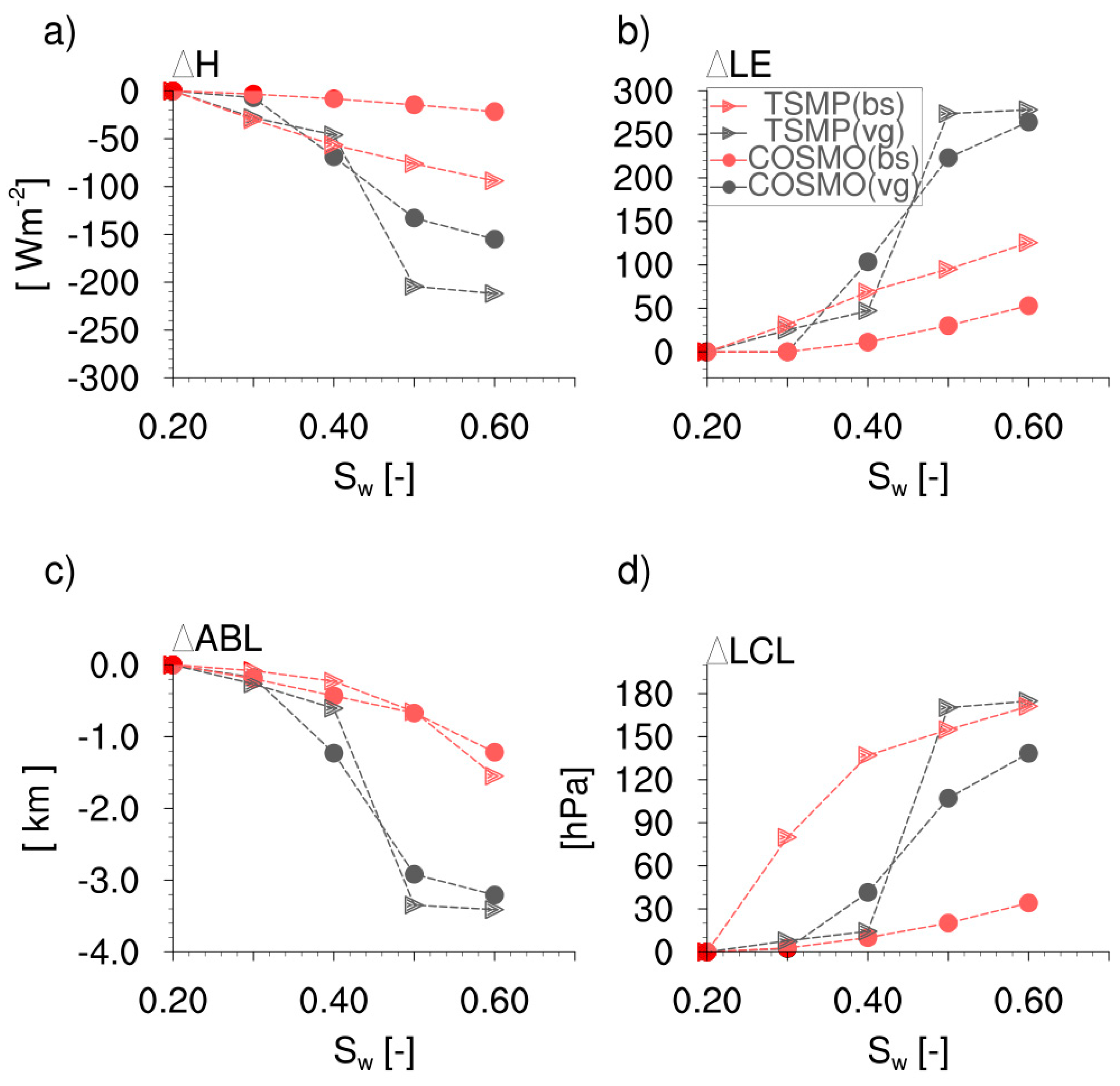
4.2.1. Surface Fluxes

Figure 4a,b show the response of the mean sensible (H) and latent heat fluxes (LE), respectively, to increasing initial soil moisture for the CSDR experiment. As expected, H decreases and LE increases monotonically with increasing initial soil moisture. For bare soil (bs, red curves) both fluxes change stronger in the TSMP than in the COSMO simulations. For the vegetated land surface (vg, black curves) the fluxes change in jumps, which happen for COSMO between initial soil saturations of 0.3 and 0.4 and in TSMP more gradually between 0.4 and 0.5. In general, the TSMP turbulent fluxes respond stronger to changes in the initial soil saturation for both bare soil and vegetation as compared to COSMO.

For bare soil, an increase in the deeper-layer soil moisture (VSDR experiments) has no effect in TSMP while COSMO exhibits small variations (not shown here). For the vegetated land surface, TSMP shows quite different model responses with and without extending the root vertical distribution to lower soil layers given the moist deep layer (Figure 5a,b). While the jump in the model response remains with the default root distribution (VSDR), it completely disappears with the extended root simulations (VSMR) and approaches the results for COSMO especially in LE for $S_w\ge 0.4$, as the roots are now able to take up water from deeper layers.

The simulated surface fluxes are–besides by soil moisture—controlled by the radiation budget at the surface, which depends on shortwave albedo, longwave emissivity, and surface temperature. Both LSMs simulate a lower albedo for the vegetated land surface as compared to bare soil. Net shortwave radiation $\left(R_{NSW}\right)$ barely changes with increasing soil moisture for the vegetated land surface (560 Wm⁻² for TSMP and 630 Wm⁻² for COSMO). It changes due to the decreasing albedo with soil moisture for bare soil in TSMP from 519 to 555 Wm⁻² and in COSMO from 600 to 618 Wm⁻². Since longwave emission of the land surface depends on its emissivity and temperature (also on the vegetation temperature for TSMP), net longwave radiation increases (becomes less negative) with increasing soil moisture (

Table 3. Averaged net long wave radiation (+ve downwards) from 1100 to 1400 LT.

${\mathit{S}}_{\mathit{w}}[-]$	0.2		0.3		0.4		0.5		0.6
$\overline{{\mathit{R}}_{\mathit{n}\mathit{e}\mathit{t}\left(\mathit{L}\mathit{W}\right)}}$	bs	vg	bs	vg	bs	vg	bs	vg	bs	vg
CSDR Experiment
COSMO	−199	−157	−196	−155	−189	−137	−182	−116	−172	−108
TSMP	−154	−151	−127	−146	−110	−142	−105	−98	−102	−96
VSDR Experiment
COSMO	−196	−137	−191	−129	−185	−116	−180	−111	−172	−108
TSMP	−154	−141	−127	−135	−110	−131	−105	−97	−102	−96
VSMR Experiment
COSMO	−196	−137	−191	−129	−185	−116	−180	−111	−172	−108
TSMP	−154	−120	−127	−106	−110	−102	−105	−97	−102	−96

). For bare soil, this increase is stronger in TSMP than in COSMO. For vegetated land, similar jumps as found for the surface fluxes happen for radiative fluxes: at $S_w=0.3$ for COSMO and at $S_w=0.4$ for TSMP. For high initial soil moistures ($S_w\ge 0.5$), net longwave radiation ($R_{NLW}$) is similar for bare-soil and vegetated land in TSMP while differences persist in COSMO. $R_{NLW}$ does not vary for TSMP due to changes in the deeper layer soil moisture for bare soil, while small variations occur for COSMO (Table 3). For the vegetated land surface, both models emit less longwave radiation from the surface (higher–less negative—$R_{NLW}$) with higher deeper-layer soil moisture because of the lower surface temperature caused by higher evapotranspiration at the expense of sensible heat. Accordingly, the deeper roots in the VSMR simulations (only TSMP) further decrease land surface (and vegetation) temperature and thus the emitted longwave radiation (higher $R_{NLW}$).

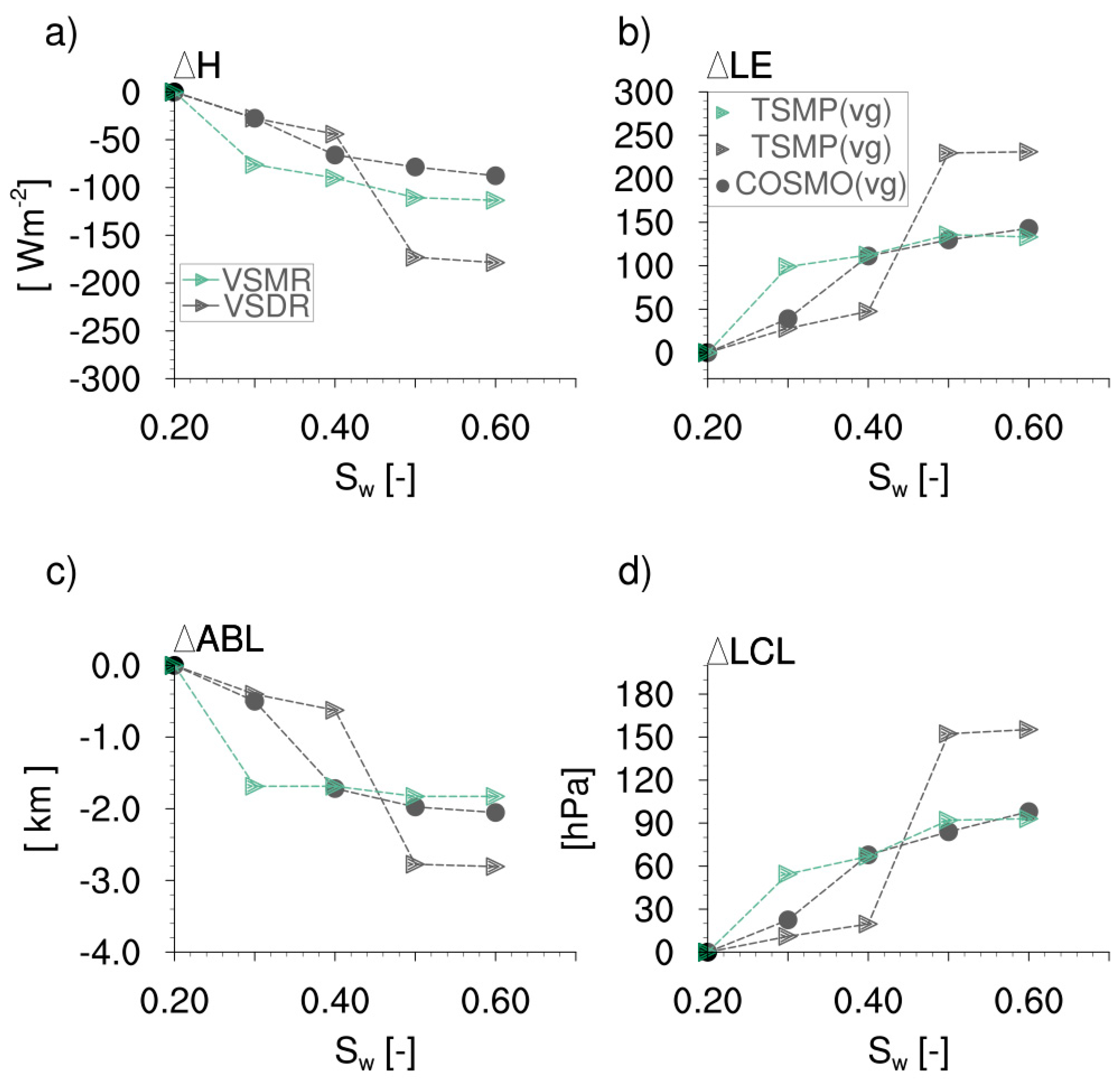
4.2.2. ABL Quantities

The flux response of both LSMs to initial soil moisture strongly impacts the ABL quantities like the virtual potential temperature and the ABL height (Figure 4c,d and Figure 5c,d). As expected, the ABL becomes cooler (not shown here) and shallower with increasing initial soil moisture. For the vegetated land surface, the model response in ABL height to initial soil moisture is larger than for bare soil. At lower soil saturation $(S_w=0.2)$, the simulated maximum ABL height for bare-soil/vegetation is approximately around 3/4 km for both models, typical for arid regions [33,34]. The higher ABL heights for vegetated surface results from its lower albedo, as explained earlier. Here, the mean ABL height in TSMP exhibits a sudden drop of approximately 2.74 km (corresponding to 3.86 K drop in ${\theta }_{v400 \mathrm{m}}$) from $S_w=0.4 \mathrm{to} 0.5$, while the COSMO mean ABL height gradually drops to similar values at high initial soil moisture. For bare soil, the mean ABL height decreases gradually with increasing soil moisture in both models. For the VSDR experiments (high available soil moisture in deeper layers) the change in ABL height over vegetated land is significantly lower corresponding to the respective $\Delta H$ decrease (Figure 5c). Jumps in $\Delta ABL$ remain more discernable in TSMP than in COSMO. In the VSMR experiment (deeper root distribution beside high available soil moisture in deeper layers), the ABL height still drops stronger in TSMP than in COSMO for $S_w=0.3$ but then converges with COSMO for $S_w\ge 0.4$.

The sensitivity of the ABL evolution to changes in soil moisture also impacts the lifting condensation level (LCL) and the convective available potential energy (CAPE). Figure 4d compares the change of the mean LCL with initial soil moisture for the two land use types for the same averaging period as ABL height. With increasing soil moisture, the mean LCL height decreases (i.e., increase in pressure) while the mean CAPE increases (not shown here). Changes are larger for TSMP as compared to COSMO, and the jumps for vegetated land surface are stronger in TSMP. In TSMP, the responses for vegetation and bare soil match at $S_w=0.6$. For the VSDR experiment, $\Delta LCL$ in both models drops for vegetation, but the jump in TSMP remains (Figure 5d). For the VSMR experiment, this jump disappears and $\Delta LCL$ converge for both models for $S_w\ge 0.4$.

5. Discussion

For both vegetated and bare soil land use, the TSMP turbulent fluxes respond stronger to initial soil moisture changes than COSMO. For bare soil, TSMP simulates much higher soil evaporation despite an additional soil resistance term and its sole dependence on the surface soil layer. The additional soil resistance decreases exponentially with increasing soil moisture and contributes to larger increase in evaporation. The impact of the deeper active layer for bare soil evaporation in COSMO is visible for shallow drier regimes (typically observed during recession periods). For very dry shallow soil moisture ($S_{w,z\le 30 \mathrm{c}\mathrm{m}}=0.2$), COSMO exhibits net loss in integrated vertical soil moisture, whereas no soil evaporation takes place in TSMP.

For vegetated lands, the characteristic jump-like response of the surface energy flux partitioning in TSMP results from a jump in the root water uptake, which depends on the available soil water for transpiration. This again depends on the soil water potential, $\psi$, and the PFT-dependent potential at which stomatas are fully open or closed in each layer (${\psi }_{close}=-2.75\times {10}^5 \mathrm{mm}\mathrm{and} {\psi }_{open}=-0.74\times {10}^5 \mathrm{mm}$). In CLM, the fraction of water available for transpiration (plant wilting factor) linearly increases from 0 to 1 between relative soil moistures of $S_w=0.43$ and $0.51$. In this range, which also depends on soil structure, the model plants experience water stress. With $\psi <{\psi }_{close}$, stomata completely close and transpiration shuts down. The soil moisture limiting functions in CLM and TERRA-ML differ as the prior is computed as an integral of plant wilting factor and fractions of roots in each layer, while the latter depends on the integrated total root zone soil moisture content. This partly explains the absence of strong jumps in model response for TERRA-ML. It also contributes to higher net loss in soil moisture for experiments with only shallow drier regimes, where all COSMO simulations lose more water ($S_{w,z\le 30 \mathrm{c}\mathrm{m}}\le 0.4$) as compared to the TSMP simulations. For shallow drier regimes, only with additional modified deeper root fraction distribution, the TSMP response tends to converge with COSMO results. In CLM, the static root fraction distribution needs to be modified to bring larger portion of root fractions to available water in deeper layers [9]. Besides, the permanent wilting point in TERRA-ML depends on the soil type, and is slightly lower than in CLM with respect to the relative soil moisture content; hence the shift between the model responses in CSDR experiments. For TERRA-ML and CLM, the average daytime LE is almost zero for $S_w<0.3$ and $S_w<0.4$ respectively; thus for $S_w<0.4$, both models respond very differently.

The different ground albedo parameterizations and stronger sensitivity of net longwave radiation to soil moisture content result in stronger increases of surface net radiation with increasing soil moisture in CLM as compared to TERRA-ML. However, the net radiation generally remains higher for TERRA-ML than CLM. For vegetation, the absence of an explicit canopy layer (and canopy radiative transfer scheme) in TERRA-ML results in a higher ground temperature and lower net longwave radiation [9,35]. For the vegetated land surface in TSMP, the experiments with deeper root fraction distribution also increase the net radiation at the ground. This indirect effect is due to the change in the partitioning of surface energy fluxes, which increases LE and reduces H. It reduces the ground temperature and increases the net longwave radiation. Earlier, it was shown that deeper root fraction distributions and soil moisture assimilation allows for improved simulations of soil states and surface energy flux partitioning for a temperate grassland site in Germany [9]. The current experiments also indicate, that the simplified assumption of an invariant vertical root distribution could lead to biases in the available root zone soil moisture in CLM. This could have an important role in the partitioning of surface energy fluxes, which could strongly impact the changes in model response.

Overall, the response of LSMs to changing soil moisture may strongly differ because of the different parameterizations for bare soil evaporation, canopy transpiration, and the soil-vegetation structure, which affects the ground albedo. Soil resistance and the soil moisture limitation factor from roots and stomatal closure are semi-empirical and depend on soil/plant dependent potentials at which stomata fully close or open, that need to be specified a priori. Our experiments show that the changes in surface energy flux partitioning strongly modulate the evolution of ABL profiles and height, LCL and CAPE. The change in ABL height and LCL in both COSMO and TSMP tends to follow the change in surface energy flux partitioning. The changes in surface and ABL quantities tends to converge for experiments with shallow dry regimes and modified root distribution between COSMO and TSMP. Variations in ABL profiles and height, LCL and CAPE due to different surface energy flux partitioning might result in quite different timings and intensities of convection initiation and precipitation in coupled modeling systems (e.g., [3,8,36,37]).

6. Conclusions

The root water uptake and bare-soil evaporation parameterization in TERRA-ML more weakly respond to changes in soil moisture as compared to CLM, which also simulates in general much higher evaporation. The nature and strength of the land-atmosphere coupling between the two LSMs was found to vary strongly for the drier regimes. The variability was found to persist even with shallow drier regimes (typically observed during recession periods). This difference was shown to be associated with the priori specification of the shallow root fraction distribution in CLM, which limits the available root zone soil moisture. Such variability could be masked if the model exhibits a wet bias [9]. However, when both models simulate soil hydrology similarly accurate in the drier regimes, they will produce different surface energy flux partitioning. This diverging tendency between the LSMs could contribute to uncertainties in understanding land-atmosphere feedback processes relevant for weather and climate simulations. The experiments designed in this work are thus crucial to identify the variability in model response when adding more physically based processes to simulate the surface characteristics. Further semi-idealized modeling studies needs to be undertaken using measurements (for periods of recession) over different vegetation types to quantify the uncertainty in the simulated land-atmosphere feedbacks.

The model responses simulated in this study will vary in extent, when different initial soundings are used to initialize the atmospheric model or when different soil-vegetation structures and vertical profiles of soil moisture are employed. We expect, however, the results can be generalized in their tendencies; thus, different model physics and parameterization in the LSMs can exert systematic differences in the range of model responses and sensitivities of ABL characteristics to similarly varying initial soil moisture contents and atmospheric soundings.

References

1. Seuffert, G.; Gross, P.; Simmer, C.; Wood, E.F. The influence of hydrologic modeling on the predicted local weather: Two-way coupling of a mesoscale weather prediction model and a land surface hydrologic model. J. Hydrometeorol. 2002, 3, 505–523. [Google Scholar] [CrossRef]
2. Jin, J.; Miller, N.L.; Schlegel, N. Sensitivity Study of Four Land Surface Schemes in the WRF Model. Adv. Meteorol. 2010, 2010, 167436. [Google Scholar] [CrossRef] [Green Version]
3. Davin, E.L.; Stöckli, R.; Jaeger, E.B.; Levis, S.; Seneviratne, S.I. COSMO-CLM2: A new version of the COSMO-CLM model coupled to the Community Land Model. Clim. Dyn. 2011, 37, 1889–1907. [Google Scholar] [CrossRef] [Green Version]
4. Chen, F.; Liu, C.; Dudhia, J.; Chen, M. A sensitivity study of high resolution regional climate simulations to three land surface models over the western United States. J. Geophys. Res. Atmos. 2014, 119, 7271–7291. [Google Scholar] [CrossRef]
5. Santanello, J.A., Jr.; Peters-Lidard, C.D.; Kennedy, A.; Kumar, S.V. Diagnosing the nature of land–atmosphere coupling: A case study of dry/wet extremes in the US southern Great Plains. J. Hydrometeorol. 2013, 14, 3–24. [Google Scholar] [CrossRef] [Green Version]
6. Shrestha, P.; Sulis, M.; Masbou, M.; Kollet, S.; Simmer, C. A scale-consistent Terrestrial System Modeling Platform based on COSMO, CLM and ParFlow. Mon. Weather Rev. 2014, 142, 3466–3483. [Google Scholar] [CrossRef]
7. Keune, J.; Gasper, F.; Goergen, K.; Hense, A.; Shrestha, P.; Sulis, M.; Kollet, S. Studying the influence of groundwater representations on land surface-atmosphere feedbacks during the European heat wave in 2003. J. Geophys. Res. Atmos. 2016, 121, 13301–13325. [Google Scholar] [CrossRef]
8. Sulis, M.; Keune, J.; Shrestha, P.; Simmer, C.; Kollet, S. Quantifying the impact of subsurface-land surface physical processes on the predictive skill of subseasonal mesoscale atmospheric simulations. J. Geophys. Res. Atmos. 2018, 123, 9131–9151. [Google Scholar] [CrossRef]
9. Shrestha, P.; Kurtz, W.; Vogel, G.; Schulz, J.-P.; Sulis, M.; Hendricks Franssen, H.-J.; Kollet, S.; Simmer, C. Connection between root zone soil moisture and surface energy flux partitioning using modeling, observations, and data assimilation for a temperate grassland site in Germany. J. Geophys. Res. Biogeosci. 2018, 123, 2839–2862. [Google Scholar] [CrossRef] [Green Version]
10. Grasselt, R.; Schüttemeyer, D.; Warrach-Sagi, K.; Ament, F.; Simmer, C. Validation of TERRA-ML with discharge measurements. Meteorol. Z. 2008, 17, 763–773. [Google Scholar] [CrossRef]
11. Doms, G.; Förstner, J.; Heise, E.; Herzog, H.-J.; Raschendorfer, M.; Reinhardt, T.; Ritter, B.; Schrodin, R.; Schulz, J.-P.; Vogel, G. A Description of the Nonhydrostatic Regional Model LM, Part II: Physical Parameterization. 2007. Available online: http://www.cosmo-model.org (accessed on 8 April 2015).
12. Schulz, J.-P.; Vogel, G.; Becker, C.; Kothe, S.; Rummel, U.; Ahrens, B. Evaluation of the ground heat flux simulated by a multi-layer land surface scheme using high-quality observations at grass land and bare soil. Meteorol. Z. 2016, 25, 607–620. [Google Scholar] [CrossRef]
13. Oleson, K.W.; Niu, G.Y.; Yang, Z.L.; Lawrence, D.M.; Thornton, P.E.; Lawrence, P.J.; Stockli, R.; Dickinson, R.E.; Bonan, G.B.; Levis, S.; et al. Improvements to the Community Land Model and their impact on the hydrological cycle. J. Geophys. Res. 2008, 113, 01021. [Google Scholar] [CrossRef]
14. Baldauf, M.; Seifert, A.; Förstner, J.; Majewski, D.; Raschendorfer, M.; Reinhardt, T. Operational convective-scale numerical weather prediction with the COSMO model: Description and sensitivities. Mon. Weather Rev. 2011, 139, 3887–3905. [Google Scholar] [CrossRef]
15. Valcke, S. The OASIS3 coupler: A European climate modelling community software. Geosci. Model Dev. 2013, 6, 373–388. [Google Scholar] [CrossRef] [Green Version]
16. Valcke, S.; Craig, T.; Coquart, L. OASIS3-MCT User Guide, OASIS3-MCT 2.0. CERFACS/CNRS SUC URA NO. 1875. Available online: http://www.cerfacs.fr/oa4web/oasis3-mct/oasis3mct_UserGuide.pdf (accessed on 8 April 2015).
17. Gasper, F.; Goergen, K.; Shrestha, P.; Sulis, M.; Rihani, J.; Geimer, M.; Kollet, S.J. Implementation and scaling of the fully coupled Terrestrial Systems Modeling Platform (TerrSysMP v1.0) in a massively parallel supercomputing environment—A case study on JUQUEEN (IBM Blue Gene/Q). Geosci. Model Dev. 2014, 7, 2531–2543. [Google Scholar] [CrossRef] [Green Version]
18. Shrestha, P.; Sulis, M.; Simmer, C.; Kollet, S. Effects of horizontal grid resolution on evapotranspiration partitioning using TerrSysMP. J. Hydrol. 2018, 557, 910–915. [Google Scholar] [CrossRef]
19. Poll, S.; Shrestha, P.; Simmer, C. Modelling convectively induced secondary circulations in the terra incognita with TerrSysMP. Q. J. R. Meteorol. Soc. 2017, 143, 2352–2361. [Google Scholar] [CrossRef] [Green Version]
20. Steppeler, J.; Doms, G.; Schättler, U.; Bitzer, H.W.; Gassmann, A.; Damrath, U.; Gregoric, G. Meso-gamma scale forecasts using the nonhydrostatic model LM. Meteorol. Atmos. Phys. 2003, 82, 75–96. [Google Scholar] [CrossRef]
21. Doms, G.; Förstner, J.; Heise, E.; Herzog, H.-J.; Mironov, D.; Raschendorfer, M.; Reinhardt, T.; Ritter, B.; Schrodin, R.; Schulz, J.-P.; et al. A Description of the Nonhydrostatic Regional Model LM, Part II: Physical Parameterization. 2011. Available online: http://www.cosmo-model.org (accessed on 23 May 2016).
22. Ritter, B.; Geleyn, J.F. A comprehensive radiation scheme for numerical weather prediction models with potential applications in climate simulations. Mon. Weather Rev. 1992, 120, 303–325. [Google Scholar] [CrossRef] [Green Version]
23. Mellor, G.L.; Yamada, T. Development of a turbulence closure model for geophysical fluid problems. Rev. Geophys. Space Phys. 1982, 20, 851–875. [Google Scholar] [CrossRef] [Green Version]
24. Blackadar, A.K. The vertical distribution of wind and turbulent exchange in neutral atmosphere. J. Geophys. Res. 1962, 67, 3095–3102. [Google Scholar] [CrossRef] [Green Version]
25. Raschendorfer, M. The new turbulence Parameterization of LM. COSMO Newslett. 2001, 1, 89–97. Available online: http://www.cosmo-model.org (accessed on 8 April 2015).
26. Dickinson, R.E. Modeling evapotranspiration for three-dimensional global climate models. Clim. Process. Clim. Sensit. Geophys. Monogr. 1984, 29, 58–72. [Google Scholar]
27. Jarvis, P.G. The interpretation of the variations in leaf water potential and stomatal conductance found in canopies in the field. Philos. Trans. R. Soc. B 1976, 273, 593–610. [Google Scholar] [CrossRef]
28. Stewart, J.B. Modelling surface conductance of pine forest. Agric. For. Meteorol. 1988, 43, 19–35. [Google Scholar] [CrossRef]
29. Sellers, P.J.; Berry, J.A.; Collatz, G.J.; Field, C.B.; Hall, F.G. Canopy reflectance, photosynthesis, and transpiration. III. A reanalysis using improved leaf models and a new canopy integration scheme. Remote Sens. Environ. 1992, 42, 187–216. [Google Scholar] [CrossRef]
30. Collatz, G.; Ball, J.T.; Grivet, C.; Berry, J.A. Physiological and environmental regulation of stomatal conductance, photosynthesis and transpiration: A model that includes a laminar boundary layer. Agric. For. Meteorol. 1991, 54, 107–136. [Google Scholar] [CrossRef]
31. Shrestha, P. TerrSysMP Pre-Processing and Post-Processing System. CRC/TR32 Database (TR32DB). Available online: https://www.tr32db.uni-koeln.de/data.php?dataID=1873 (accessed on 28 March 2019).
32. John, J.A.; Draper, N.R. An alternative family of transformations. Appl. Stat. 1980, 29, 190–197. [Google Scholar] [CrossRef]
33. Garratt, J.R. The atmospheric boundary layer. Earth-Sci. Rev. 1994, 37, 89–134. [Google Scholar] [CrossRef]
34. Ma, M.; Pu, Z.; Wang, S.; Zhang, Q. Characteristics and numerical simulations of extremely large atmospheric boundary-layer heights over an arid region in north-west China. Bound.-Layer Meteorol. 2011, 140, 163–176. [Google Scholar] [CrossRef]
35. Vogel, G.; Shrestha, P.; Schulz, J.-P.; Becker, C.; Rummel, U. Modelluntersuchungen zum Einfluss der Abschattung der Solarstrahlung durch die Vegetation auf die Erdbodentemperaturen in Falkenberg. MOL-RAO Aktuell. Available online: http://www.dwd.de/DE/forschung/atmosphaerenbeob/lindenbergersaeule/publikationen/publikationen_node.html (accessed on 1 September 2015).
36. Davin, E.L.; Maisonnave, E.; Seneviratne, S.I. Is land surface processes representation a possible weak link in current Regional Climate Models? Environ. Res. Lett. 2016, 11, 074027. [Google Scholar] [CrossRef]
37. Sulis, M.; Williams, J.L.; Shrestha, P.; Diederich, M.; Simmer, C.; Kollet, S.; Maxwell, R.M. Coupling Groundwater, Vegetation, and Atmospheric Processes: A Comparison of Two Integrated Models. J. Hydrometeorol. 2017, 18, 1489–1511. [Google Scholar] [CrossRef]
38. Simmer, C.; Thiele-Eich, I.; Masbou, M.; Amelung, W.; Bogena, H.; Crewell, S.; Diekkrüger, B.; Ewert, F.; Hendricks Franssen, H.-J.; Huisman, J.A.; et al. Monitoring and modeling the terrestrial system from pores to catchments—The transregional collaborative research center on patterns in the soil-vegetation-atmosphere system. Bull. Am. Meteorol. Soc. 2014, 96, 1765–1787. [Google Scholar] [CrossRef] [Green Version]
Figure 1. Vertical profile of the change in soil moisture content ( Δ η ) for the CSDR (Vertically Constant Relative Soil Saturation and Default Root Distribution) experiment with initial soil moisture contents from 0.2 to 0.6 (columns 2–6) for bare soil (upper row) and vegetated land (lower row). The first column shows the common vertically constant profile of the initial soil moisture content dependent on magnitude of S w (top) and the CLM (Community Land Model) root fraction distribution including the TERRA-ML (TERRA Multi Layer) root depth (bottom).
Water 12 00046 g001
Figure 2. Vertical profile of the change in soil moisture content ( Δ η ) for the VSDR (Vertically Varying Relative Soil Saturation and Default Root Distribution) experiment with initial soil moisture contents from 0.2 to 0.6 (columns 2–6) for bare soil (upper row) and vegetated land (lower row). The first column shows the common vertically varying profile of the initial soil moisture content dependent on magnitude of S w (top) and the CLM root fraction distribution including the TERRA-ML root depth (bottom).
Water 12 00046 g002
Figure 3. Vertical profile of the change in soil moisture content ( Δ η ) for the VSMR (Vertically Varying Relative Soil Saturation and Modified Root Distribution) experiment with initial soil moisture contents from 0.2 to 0.6 (columns 2–6) for bare soil (upper row) and vegetated land (lower row). The first column shows the common vertically varying profile of the initial soil moisture content dependent on magnitude of S w (top) and the CLM root fraction distribution including the TERRA-ML root depth (bottom).
Water 12 00046 g003
Figure 4. Model response of surface fluxes and boundary layer mean quantities for CSDR experiment: (a) Sensible heat flux ( Δ H ) , (b) Latent heat flux ( Δ L E ) , (c) Virtual potential temperature ( Δ   θ v ) .
Water 12 00046 g004
Figure 5. Response of the surface fluxes and boundary layer mean quantities to increasing near surface soil saturation ( S w ) for VSDR experiment: (a) Sensible heat flux ( Δ H ) , (b) Latent heat flux ( Δ L E ) , (c) Virtual potential temperature ( Δ   θ v ) around 400 m a.g.l., and (d) Lifting Condensation Level ( Δ L C L ) . TSMP results are also shown for VSMR experiment (green marked lines).
Water 12 00046 g005