Comparison of Bootstrap Confidence Intervals Using Monte Carlo Simulations

Abstract

Design of hydraulic works requires the estimation of design hydrological events by statistical inference from a probability distribution. Using Monte Carlo simulations, we compared coverage of confidence intervals constructed with four bootstrap techniques: percentile bootstrap (BP), bias-corrected bootstrap (BC), accelerated bias-corrected bootstrap (BCA) and a modified version of the standard bootstrap (MSB). Different simulation scenarios were analyzed. In some cases, the mother distribution function was fit to the random samples that were generated. In other cases, a distribution function different to the mother distribution was fit to the samples. When the fitted distribution had three parameters, and was the same as the mother distribution, the intervals constructed with the four techniques had acceptable coverage. However, the bootstrap techniques failed in several of the cases in which the fitted distribution had two parameters.

1. Introduction

In the study and design of hydraulic works, hydrological events must be estimated by statistical inference [1,2] as predetermined quantiles from a probability distribution [3,4]. A quantile is defined as a magnitude of a hydroclimatological variable (precipitation, flow, etc.) associated with a return period. The return period is the average time interval in which said magnitude is reached or surpassed [5].

In hydrology, it is not enough to obtain the value of an event associated with a return period since there is a level of uncertainty in the estimation of parameters and quantiles from finite samples [6], which must be considered in decision-making [7]. One way to report this uncertainty is to provide an interval that has a high likelihood of including the true value of the quantity of interest. Said interval is known as the confidence interval, and the likelihood that it contains the true value is known as the confidence level. As the uncertainty increases, so does the width of the confidence interval [8,9].

Traditionally, confidence intervals are obtained from a parametric estimator of the standard error $s$ of a quantity of interest $\theta$. A confidence interval of 95%, then, is obtained by adding or subtracting the standard error multiplied by a critical value (for example, $\theta \pm 1.96\mathrm{s}$). This calculation assumes that the distribution of the estimator of $\theta$ is approximately normal [6,10].

There are various situations in which the assumption of normality is incorrect. In these cases, or when the standard error is very difficult to estimate, one alternative is to use techniques based on bootstrap re-sampling [3,6,11]. In bootstrap resampling, proposed by [12], the distribution of a given statistic is inferred from the available data [8,13]. For this purpose, many samples are generated from the original sample using Monte Carlo simulations. There are two basic approaches for the bootstrap: parametric and non-parametric re-sampling. In parametric resampling, random samples are generated from a parametric model fit to the data. In non-parametric resampling, the bootstrap samples are constructed using the resampling with replacement from the original sample [14,15]. The parametric bootstrap is very similar to Monte Carlo simulation. The difference is that the parameters used for the parametric bootstrap are estimated from the sample, whereas the parameters for the Monte Carlo simulation are set, based on the purposes of the simulation. Thus, a Monte Carlo simulation would be used for a theoretical study, whereas the parametric bootstrap would be used to make statistical inference from sampled data. In terms of implementation, the parametric bootstrap and Monte Carlo simulation are the same [16].

Regardless of the approach used to generate the bootstrap samples, the construction of the confidence intervals requires calculating the quantity of interest for each of the bootstrap samples and, later, from the calculated values, estimating the confidence limits using order statistics [17,18].

There is a variety of techniques for constructing confidence intervals from bootstrap samples. Among these are the percentile bootstrap (BP), the bias-corrected bootstrap (BC), the accelerated bias-corrected bootstrap (BCA) and the standard bootstrap (SB). All of these techniques have their advantages and disadvantages [8]. However, it is not clear which is convenient for constructing confidence intervals for quantiles of hydroclimatological variables. One way to verify whether a technique for the construction of confidence intervals is effective is to calculate the coverage of the intervals constructed using that technique. Coverage is defined as the percentage of times in which the confidence intervals include the true value of the quantity of interest. This coverage should coincide with the confidence level of the interval. That is, for a confidence level of 95%, it is expected that 95% of the confidence intervals contain the true value of the quantity of interest [19,20].

The aim of this study was to compare the coverage of the confidence intervals obtained with four bootstrap techniques under different simulation scenarios, analyzing series of 24-h annual maximum precipitation. The bootstrap techniques are the percentile bootstrap, the bias-corrected bootstrap, the accelerated bias-corrected bootstrap and a modification of the standard bootstrap that we propose here.

2. Materials and Methods

2.1. Climatological Information

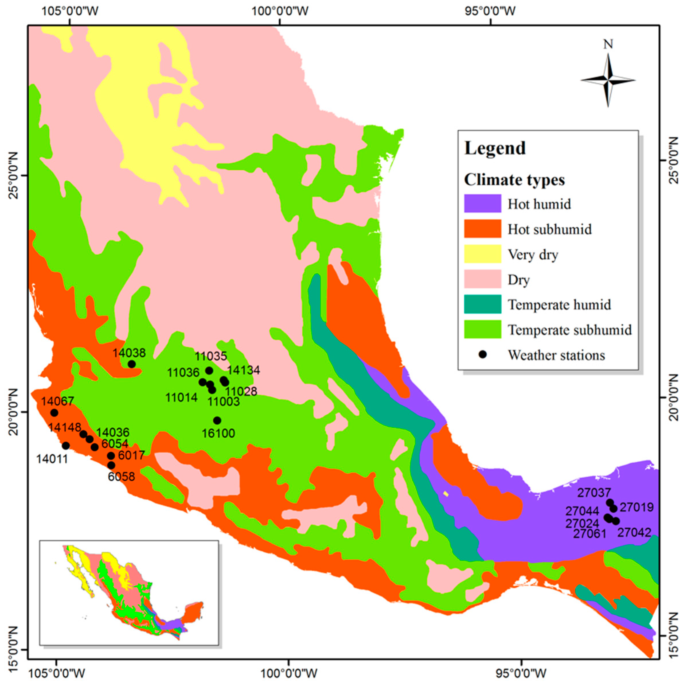
The data used in this study were 24-h annual maximum precipitation records obtained from 21 meteorological stations in Mexico (Figure 1) from the National Climatological Database (CLICOM-Climate Computing) (http://smn.cna.gob.mx/index.php?option=com_content&view=article&id=42&Itemid=75) [21]. The records vary from 32 to 89 years for the period from 1923 to 2012. The stations are found in five states and in three different climate types (Table 1).

Figure 1. Location of the meteorological stations used in this study.

Table 1. Geographic location and information from the meteorological stations used in the study.

Station	Name	Climate Type	Latitude (° N)	Longitude (° E)	Altitude (masl)	Period of Records	Mean (mm)	Standard Deviation	Skewness Coefficient
6017	Madrid	Hot subhumid	19.1122	−103.8839	195	1970–2012	112	65.4	2.38
6054	M. Á. Camacho	Hot subhumid	19.285	−104.245	376	1978–2012	107	62.3	2.02
6058	Tecomán	Hot subhumid	18.9083	−103.8744	30	1954–2012	112	62.2	1.35
14011	Apazulco	Hot subhumid	19.3064	−104.8875	5	1961–2011	126	62.1	0.9
14036	Cuautitlán	Hot subhumid	19.4506	−104.3592	600	1958–2011	115	50.9	2.08
14067	Higuera Blanca	Hot subhumid	19.9942	−105.1625	140	1956–2002	111	68	1.29
14148	Tecomates	Hot subhumid	19.5583	−104.5	286	1961–2006	102	32	1.16
11003	Agua Tibia	Temperate subhumid	20.5103	−101.6294	1720	1949–2012	53.2	15.7	0.295
11014	Cuerámaro	Temperate subhumid	20.6256	−101.6758	1732	1967–2012	49.4	16.8	−0.16
11028	Irapuato	Temperate subhumid	20.6689	−101.3372	1729	1923–2011	53.8	16.5	1.55
11035	La Sandía	Temperate subhumid	20.9211	−101.6974	1771	1965–2012	52.9	16.3	−0.31
11036	Adjuntas	Temperate subhumid	20.6753	−101.8442	1727	1944–2012	54	19.3	1.64
11134	El Conejo	Temperate subhumid	20.7158	−101.3697	1740	1978–2012	54.9	15.1	0.586
14038	Cuixtla	Temperate subhumid	21.0519	−103.4389	1000	1954–2011	57.5	13.9	0.65
16100	P. San Isidro	Temperate subhumid	19.8658	−101.5189	2022	1947–1992	46.4	10.2	0.73
27019	Jalapa	Hot humid	17.7233	−92.8117	14	1971–2012	161	44.5	0.939
27024	La Huasteca	Hot humid	17.52	−92.9267	80	1970–2012	150	53.4	1.59
27037	P. Nuevo	Hot humid	17.8542	−92.8792	21	1949–2012	127	46.8	1.33
27042	Tapijulapa	Hot humid	17.4611	−92.7775	44	1962–2012	200	66.9	0.417
27044	Teapa	Hot humid	17.5489	−92.9533	51	1960–2012	178	44.1	0.891
27061	Puyacatengo	Hot humid	17.5133	−92.92	86	1972–2012	193	62.7	1.36

2.2. Simulation Software

We used Scilab 5.4.1 (http://www.scilab.org), an open source scientific software. Scilab is a high level programming language which includes a library of around 2000 defined functions. In Scilab, matrices are the fundamental object for scientific calculations. Thus, Scilab programs are compact and usually smaller to their equivalents in C, C++, or Java.

2.3. Bootstrap Techniques

We compared four bootstrap techniques for construction of confidence intervals: the percentile bootstrap (BP), the bias-corrected bootstrap (BC), the accelerated bias-corrected bootstrap (BCA) and a modification of the standard bootstrap (MSB).

2.3.1. Percentile Bootstrap (BP)

The BP interval is just the interval between the $100\left(\frac{\alpha }{2}\right)$ and $100\left(1-\frac{\alpha }{2}\right)$ percentiles of the distribution of estimates of $x_T$ from each resample. BP confidence intervals are based on the assumption that there exists a monotone transformation $\widehat{\varphi }=h({\widehat{x}}_T), \varphi =h(x_T)$ such that $\widehat{\varphi } ~ N(\varphi , {\tau }^2)$ (the transformed variable $\widehat{\varphi }$ follows a normal distribution with mean $\varphi$ and variance ${\tau }^2$), where $\tau$ is constant, $x_T$ represents the true value of the quantile associated to the return period $T$, ${\widehat{x}}_T$ is an estimator of $x_T$, and $h$ is a normalizing transformation. It can be verified that, for the transformed variable, the BP intervals are correct, that is, their coverage probability is exactly $100(1-\alpha )\%$, as claimed. BP intervals are transformation invariant, which means that if they are correct on the transformed scale $\varphi =h(x_T)$, then they must also be correct on the original scale $x_T$. The BP method automatically incorporates the normalizing transformation $h$, so knowledge of this transformation is not required to implement the method, but it must exist for the BP intervals to be correct [14,22].

To construct a confidence interval of $100(1-\alpha )\%$ with the BP method, for the quantile $x_T$ corresponding to a $T$ return period, the following procedure was carried out: (1) $\mathrm{B}$ random samples of the mother distribution are generated; (2) for each of the random samples, the parameters of the distribution function fit to the data are estimated, and then the quantiles; (3) the quantiles of all the samples are ordered from lowest to highest, and (4) the confidence interval is constructed in the following form:

$$\left[x_{Tj}^{\ast };x_{Tk}^{\ast }\right]$$

(1)

where $x_{Tj}^{\ast }$ represents the jth quantile of the set of ordered quantiles from lowest to highest; $x_{Tk}^{\ast }$ represents the kth quantile of the same set, $j=\left[\frac{\alpha }{2}(B+1)\right]$, $k=\left[\left(1-\frac{\alpha }{2}\right)(B+1)\right]$; and $\alpha$ is the level of significance. We used $\mathrm{B}=1999$ and $\alpha =0.05$; the quantile corresponding to the lower limit of the interval was $x_{Tj}^{\ast }=x_{T 50}^{\ast }$ (the 50th quantile) and that corresponding to the upper limit was $x_{Tk}^{\ast }=x_{T 1950}^{\ast }$ (the 1950th quantile).

2.3.2. Bias-Corrected Bootstrap (BC)

When the estimator ${\widehat{x}}_T$ is biased, a transformation $\widehat{\varphi }=h({\widehat{x}}_T)$ such that $\widehat{\varphi }\sim N(\varphi ,{\tau }^2)$ does not exist and BP intervals are not accurate [14,23]. Efron [24,25] introduced a modification of the BP method which incorporated a bias correction factor ${\mathrm{z}}_0$. This factor is estimated using the expression ${\mathrm{z}}_0={\Phi }^{-1}\left({\widehat{F}}_b({\widehat{x}}_T)\right)$, in which $\Phi$ is the standard normal distribution function and ${\widehat{F}}_b$ is the empirical probability of the estimated quantile ${\widehat{x}}_T$ (Equation (2)).

$${\widehat{F}}_b=P(x_{Ti}^{\ast }<{\widehat{x}}_T)=\frac{m}{B}$$

(2)

where $m$ is the number of bootstrap quantiles smaller than ${\widehat{x}}_T$. The quantile ${\widehat{x}}_T$ is that estimated from the data of the original sample; it should not be confused with the bootstrap quantiles $x_{Ti}^{\ast }$ estimated from the random samples.

If ${\mathrm{z}}_0$ is known, the values of $a_1$ and $a_2$ are obtained:

$$a_1=\Phi \left(2{\mathrm{z}}_0+{\mathrm{z}}_{\frac{\alpha }{2}}\right)$$

(3)

$$a_2=\Phi \left(2{\mathrm{z}}_0+{\mathrm{z}}_{1-\frac{\alpha }{2}}\right)$$

(4)

where ${\mathrm{z}}_{\frac{\alpha }{2}}$ and ${\mathrm{z}}_{1-\frac{\alpha }{2}}$ are the percentiles $100\left(\frac{\alpha }{2}\right)$ and $100\left(1-\frac{\alpha }{2}\right)$ of a standard normal distribution, respectively. For $\alpha =0.05$ (95% confidence level) ${\mathrm{z}}_{\frac{\alpha }{2}}={\mathrm{z}}_{0.025}=-1.96$ y ${\mathrm{z}}_{1-\frac{\alpha }{2}}={\mathrm{z}}_{0.975}=1.96$.

When ${\mathrm{a}}_1$ and ${\mathrm{a}}_2$ are known, the confidence interval is constructed as in Equation (1):

$$\left[x_{Tj}^{\ast };x_{Tk}^{\ast }\right]$$

(5)

where $x_{Tj}^{\ast }$ is the j^th quantile of the set of quantiles ordered from lowest to highest, $x_{Tk}^{\ast }$ represents the k^th quantile of the same set, $j=a_1(B+1)$ and $k=a_2(B+1)$.

The bias-corrected (BC) bootstrap method assumes that there is a monotone transformation $\widehat{\varphi }=h({\widehat{x}}_T), \varphi =h(x_T)$ such that $\widehat{\varphi }\sim N(\varphi -{\mathrm{z}}_0\tau , {\tau }^2)$, where ${\mathrm{z}}_0$ and $\tau$ are constant [14]. Efron [25] has shown that when such a transformation exists, BC intervals are correct. When ${\mathrm{z}}_0=0$, the BC confidence intervals are equivalent to the BP intervals.

2.3.3. Accelerated Bias-Corrected Bootstrap (BCA)

Efron [26] introduced an improvement of the BC method which corrects for both bias and skewness. This bias-corrected and accelerated (BCA) method requires calculation of a bias correction factor ${\mathrm{z}}_0$ and of an acceleration factor $a$. The coefficient ${\mathrm{z}}_0$ is calculated in the same way as in the BC technique. The $a$ coefficient can be obtained by jacknife resampling [8]. This involves generating $n$ number of replicates of the original sample, where $n$ is the number of observations in said sample. The first jackknife replicate is obtained by leaving out the first value of the original sample, the second by leaving out the second value, and so on, until $n$ samples of size $n-1$ are obtained. For each of the samples, the quantile $x_{T(-i)}$ corresponding to the return period of interest is estimated. The average of these quantities is:

$${\overline{x}}_{T(-)}=\frac{1}{n}{{\displaystyle \sum }}_{i=1}^n{x}_{T(-i)}$$

(6)

The acceleration factor $\mathrm{a}$ is calculated with Equation (7):

$$a=\frac{{{\displaystyle \sum }}_{i=1}^n{[x_{T(-i)}-{\overline{x}}_{T(-)}]}^3}{6{\left\{{{\displaystyle \sum }}_{i=1}^n{[x_{T(-i)}-{\overline{x}}_{T(-)}]}^2\right\}}^{\frac{3}{2}}}$$

(7)

With the values of ${\mathrm{z}}_0$ and $a,$ the values $a_1$ and $a_2$ are calculated:

$$a_1=\Phi \left\{{\mathrm{z}}_0+\frac{{\mathrm{z}}_0-{\mathrm{z}}_{1-\frac{\alpha }{2}}}{1-a\left({\mathrm{z}}_0-{\mathrm{z}}_{1-\frac{\alpha }{2}}\right)}\right\}$$

(8)

$$a_2=\Phi \left\{{\mathrm{z}}_0+\frac{{\mathrm{z}}_0+{\mathrm{z}}_{1-\frac{\alpha }{2}}}{1-a\left({\mathrm{z}}_0-{\mathrm{z}}_{1-\frac{\alpha }{2}}\right)}\right\}$$

(9)

where ${\mathrm{z}}_{1-\frac{\alpha }{2}}$ is the percentile $100\left(1-\frac{\alpha }{2}\right)$ of a standard normal distribution. For an $\alpha =0.05$ significance level, the percentile ${\mathrm{z}}_{1-\frac{\alpha }{2}}=1.96$. With the values of $a_1$ and $a_2$, a confidence interval is constructed in the same way as Equations (1) and (5):

$$\left[x_{Tj}^{\ast };x_{Tk}^{\ast }\right]$$

(10)

where $j=a_1(B+1)$ and $k=a_2(B+1)$.

The BCA method is based on the assumption that there is a monotone transformation $\widehat{\varphi }=h({\widehat{x}}_T), \varphi =h(x_T)$ which satisfies to a high degree of approximation $\widehat{\varphi }\sim N\left(\widehat{\varphi }-{\mathrm{z}}_0{\tau }_{\varphi },{\tau }_{\varphi }^2\right)$, where ${\tau }_{\varphi }=1+a\varphi$, and ${\mathrm{z}}_0$ and $a$ are constants [14]. Efron [27] showed that such a transformation does exist. When the acceleration coefficient $a=0$, the BCA intervals are equivalent to BC [23].

2.3.4. Modified Standard Bootstrap (MSB)

According to the standard or Gaussian bootstrap method, the confidence interval of $100(1-\mathsf{\alpha })\%$ for a quantile $x_T$ takes the form of Equation (11):

$$\left[{\widehat{x}}_T-\left({\mathrm{z}}_{1-\frac{\alpha }{2}}\right){\sigma }_b; {\widehat{x}}_T+\left({\mathrm{z}}_{1-\frac{\alpha }{2}}\right){\sigma }_b\right]$$

(11)

where ${\widehat{x}}_T$ is the estimated value of the quantile, ${\mathrm{z}}_{1-\frac{\alpha }{2}}$ is the percentile $100(1-\alpha )\%$ of a standard normal distribution, and ${\sigma }_b$ is a bootstrap estimator of the standard deviation. This estimator ${\sigma }_b$ is given by Equation (12).

$${\sigma }_b=\sqrt{\frac{1}{B-1}{{\displaystyle \sum }}_{i=1}^B{(x_{Ti}^{\ast }-{\overline{x}}_T^{\ast })}^2}$$

(12)

where $x_{Ti}^{\ast }$ is the ith bootstrap quantile and ${\overline{x}}_T^{\ast }$ is the average of the bootstrap quantiles.

We did not use the standard bootstrap in this study, but instead we propose a modification of this technique. This modification consists of constructing the standard confidence interval, not for the quantile, but for a transformation of the quantile.

The standard bootstrap method assumes that the sampling distribution of ${\widehat{x}}_T$ is normal, with mean $x_T$ and variance ${\sigma }^2$, where $\sigma$ is constant. If this assumption is not true, the standard bootstrap intervals will not be accurate [14]. However, in many cases, a transformation that stabilizes the variance will also give a variable which is closer to a normal distribution [28]. If the transformed variable is normally distributed, then the MSB will give the correct intervals.

To find an appropriate transformation, bootstrap samples were generated. The variance of the $x_{Ti}^{\ast }$ (the bootstrap estimates of $x_T$) was then expressed as a function of the mean of the $x_{Ti}^{\ast }$ using a linear regression. A transformation was then chosen which would give nearly constant variance for the transformed data. This transformation was not the same if the data were generated from a two-parameter distribution or from a three-parameter distribution. Therefore, the MSB technique varies slightly, depending on the number of parameters of the probability distribution function (pdf) fit to the time series. In the case of a three-parameter distribution, the procedure is the following: (1) the bootstrap quantiles $x_{Ti}^{\ast }$ corresponding to a return period $T$ are estimated; (2) for each of these quantiles, the transformation $u_{Ti}^{\ast }=1/x_{Ti}^{\ast }$ is performed for each of the quantiles; (3) the standard deviation of the transformed values is obtained (Equation (13)); (4) the confidence interval for $u_T=1/x_T$ is constructed, with a lower limit $UI=\frac{1}{{\widehat{x}}_T}-\left({\mathrm{z}}_{1-\frac{\alpha }{2}}\right){\sigma }_{uT}$, and an upper limit $US=\frac{1}{{\widehat{x}}_T}+\left({\mathrm{z}}_{1-\frac{\alpha }{2}}\right){\sigma }_{uT}$ (Equation (14)); (5) finally, the inverse transformation is applied to obtain a confidence interval for $x_T$, with a lower limit $XI=1/US$ and an upper limit $XS=1/UI$ (Equation (15)).

$${\sigma }_{uT}=\sqrt{\frac{1}{B-1}{{\displaystyle \sum }}_{i=1}^B{(u_{Ti}^{\ast }-{\overline{u}}_T^{\ast })}^2}$$

(13)

where ${\overline{u}}_T^{\ast }$ is the mean of the values $u_{Ti}^{\ast }$.

$$\left[\frac{1}{{\widehat{x}}_T}-\left({\mathrm{z}}_{1-\frac{\alpha }{2}}\right){\sigma }_{uT}; \frac{1}{{\widehat{x}}_T}+\left({\mathrm{z}}_{1-\frac{\alpha }{2}}\right){\sigma }_{uT}\right]$$

(14)

$$\left[{\left\{\frac{1}{{\widehat{x}}_T}+\left({\mathrm{z}}_{1-\frac{\alpha }{2}}\right){\sigma }_{uT}\right\}}^{-1};{\left\{\frac{1}{{\widehat{x}}_T}-\left({\mathrm{z}}_{1-\frac{\alpha }{2}}\right){\sigma }_{uT}\right\}}^{-1}\right]$$

(15)

It should be mentioned that, when the transformation is applied, the order of the limits is inverted. That is, the reciprocal of the upper limit US for the transformed variable $u_T$ becomes the lower limit XI for $x_T$ and the reciprocal of the lower limit UI for $u_T$ becomes the upper limit XS for $x_T$.

The procedure to obtain the interval for a two-parameter pdf is similar, except that the transformation used is $u_{Ti}^{\ast }=1/\sqrt{x_{Ti}^{\ast }}$. Later, once the confidence interval is obtained for $u_T$, the transformation $XI=1/{(US)}^2$ and $XS=1/{(UI)}^2$ must be done to obtain the confidence interval of . This interval is given by Equation (16).

$$\left[{\left\{\frac{1}{\sqrt{{\widehat{x}}_T}}+\left({\mathrm{z}}_{1-\frac{\alpha }{2}}\right){\sigma }_{uT}\right\}}^{-2};{\left\{\frac{1}{\sqrt{{\widehat{x}}_T}}-\left({\mathrm{z}}_{1-\frac{\alpha }{2}}\right){\sigma }_{uT}\right\}}^{-2}\right]$$

(16)

For a significance level $\alpha =0.05$, the percentile ${\mathrm{z}}_{1-\frac{\alpha }{2}}=1.96$.

2.4. Modeling the Coverage of Confidence Intervals

The criterion used to compare bootstrap techniques was coverage of the confidence intervals obtained by those techniques. Coverage was calculated considering two or three simulation scenarios that consider different pdf and return periods. Scenario 1 corresponds to the use of the best fitting pdf (mother distribution). Scenario 2 corresponds to modeling the second best fitting pdf. Scenario 3 corresponds to modeling the pdf which is of the same family as the mother distribution. When the second best fitting distribution is of the same family as the mother distribution, there are only two scenarios. The scenarios were obtained by generating samples of a known pdf and then fitting different pdf and estimating the quantiles using those pdfs. For each of these scenarios, confidence intervals were constructed using the four bootstrap techniques and their coverage was calculated.

The reason for this approach is the following: in practice, the real distribution of extreme rainfalls is not known, so it must be inferred from samples of finite size. Therefore, it is not unlikely that there will be cases in which inappropriate pdf are used to model the extreme rainfalls. With this in mind, some simulation scenarios were considered in which an incorrect pdf was deliberately chosen to fit the simulated data, in order to study the effect that such a choice would have on the confidence intervals. However, since it was desired that this choice of pdf, although incorrect, was still reasonable, the second best fitting pdf and the pdf of the same family as the mother distribution were considered for this purpose.

2.5. Procedure for Determining the Level of Coverage

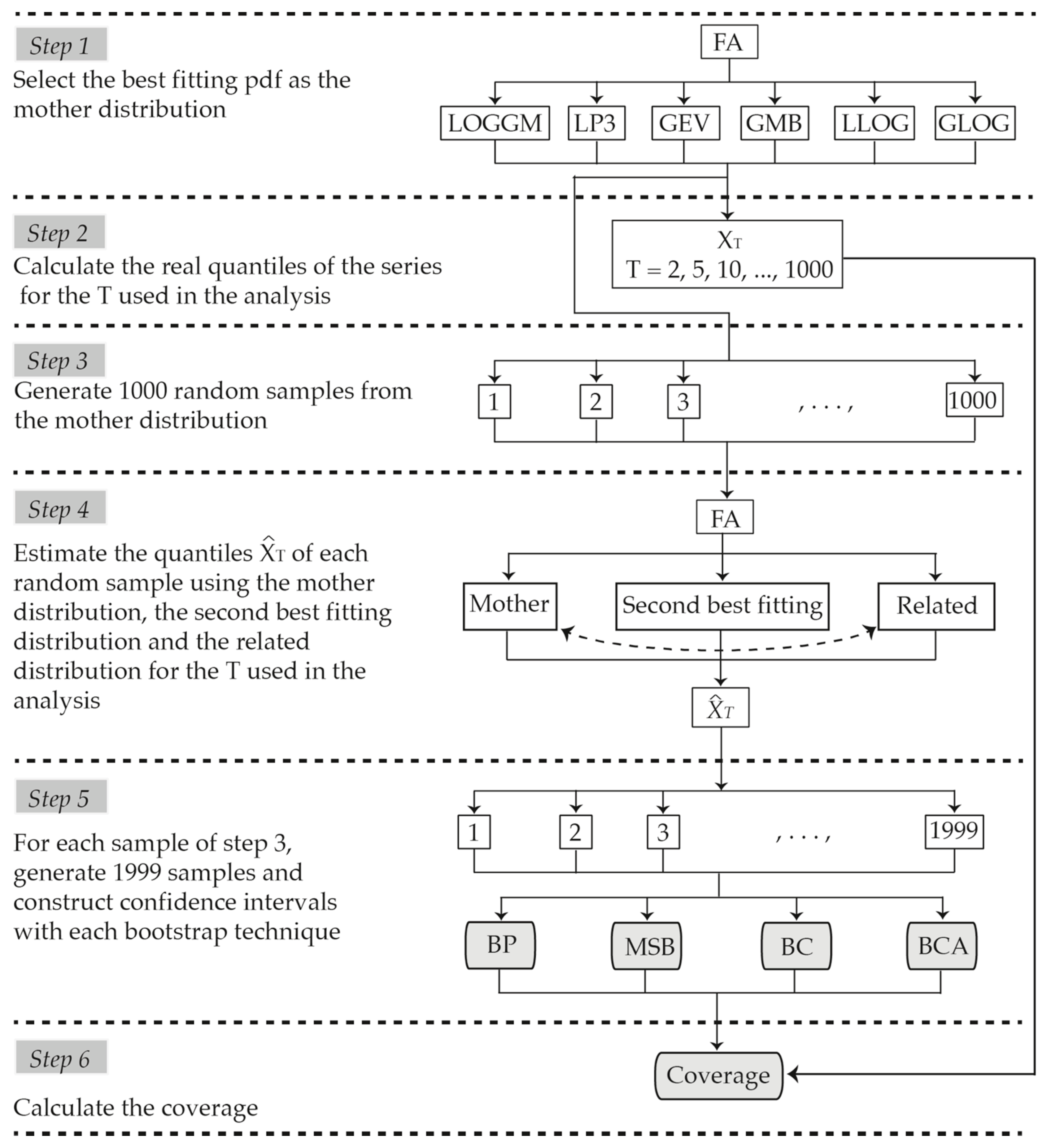
The general procedure for calculating the coverage of confidence intervals is outlined by Van de Boogard and Hall [20]. This general procedure is followed in this study, and applied to the different simulation scenarios that were considered. The methodological process used here can be summarized in the following six steps (Figure 2):

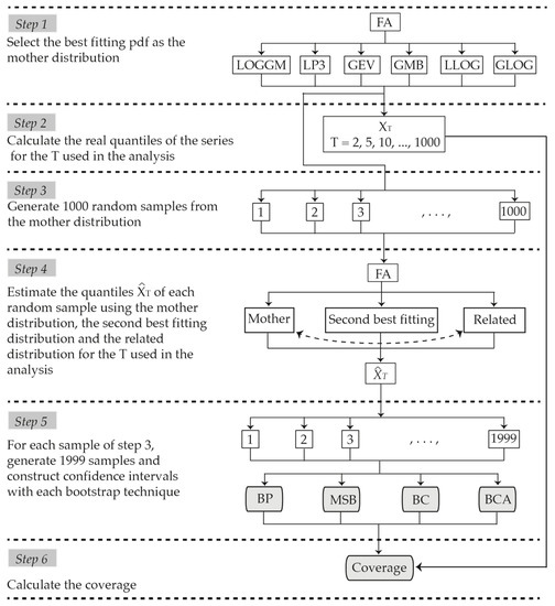
Figure 2. Methodological process for obtaining the coverage of the confidence intervals.

• Select the pdf (mother distribution) to generate the random data.
  The mother distribution for each site was selected by determining the best fitting pdf to the series of precipitation among a group of six candidates which included both two and three parameter pdf. The pdf used were log-gamma (LOGGM) and log-Pearson type 3 (LP3), Gumbel (GMB) and General Extreme Values (GEV), and log-logistic (LLOG) and generalized logistic (GLOG). The LP3, GLOG, GEV and GMB are among the most commonly used distributions for frequency analysis of extreme rainfalls [29]. The LOGGM and LLOG are two-parameter distributions related to the three parameter LP3 and GLOG distributions, respectively, as the GMB is related to the GEV. Thus, pairs of related two and three-parameter distributions were considered, allowing for the more parsimonious model to be chosen when it provided an adequate fit.
  Selection of the pdf that best fit the original and simulated series was done by applying the Bayesian Information Criterion (BIC) [30], which assigns a numerical value to each distribution that orders them from best to worst fit. In all cases, the best fitting pdf was selected for the simulations.
• Calculate the “true value” $x_T$ of the quantile for different return periods $T$.
  Quantiles corresponding to the return periods $T=$ 2, 5, 10, 20, 25, 50, 100, 200, 500 and 1000 years were estimated from the original data. These were considered as the true values of the quantiles in the simulations. The quantiles of the GMB, GEV, LLOG and GLOG pdf were calculated with Equations (17)–(20), respectively, where $\widehat{\beta }$, $\widehat{\theta }$, and $\widehat{\alpha }$ are the estimators of the scale, shape and location parameters of the distributions.

  $${\widehat{x}}_T=\widehat{\theta }-\widehat{\beta }\ln \left[\ln \left(\frac{T}{T-1}\right)\right]$$

  (17)

  $${\widehat{x}}_T=\widehat{\theta }-\frac{\widehat{\beta }}{\widehat{\alpha }}\left\{1-{\left[\ln \left(\frac{T}{T-1}\right)\right]}^{-\widehat{\alpha }}\right\}$$

  (18)

  $${\widehat{x}}_T=exp\{\widehat{\theta }+\widehat{\beta }\ln (T-1)\}$$

  (19)

  $${\widehat{x}}_T=\widehat{\theta }+\frac{\widehat{\beta }}{\widehat{\alpha }}[1-{(T-1)}^{-\widehat{\alpha }}]$$

  (20)
  No analytical forms exist for the inverse LOGGM or LP3 pdf. However, in these cases, we used SCILAB, which calculates the inverse function of the gamma distribution using the algorithm described by [31] and which served as the basis for calculating the quantiles of the LOGGM and LP3 distributions.
• Generate synthetic samples.
  One thousand synthetic samples of size $n$ were generated from the mother distribution for each of the series that were analyzed.
• Estimate the quantiles ${\widehat{x}}_{Ti}$.
  For each of the samples generated, a pdf was fitted to estimate the quantiles ${\widehat{x}}_{Ti}$ corresponding to the return periods analyzed.
• Construct confidence intervals.
  Confidence intervals were constructed for the quantiles ${\widehat{x}}_{Ti}$ with the BP, BC, BCA and MSB techniques. By generating 1000 synthetic samples, 1000 BP, 1000 BC, 1000 BCA and 1000 MSB intervals were obtained for each return period.
• Calculate coverage.
  Coverage was calculated as the percentage of times in which the intervals constructed by a bootstrap technique included the real value $x_T$ of the quantile.

3. Results and Discussion

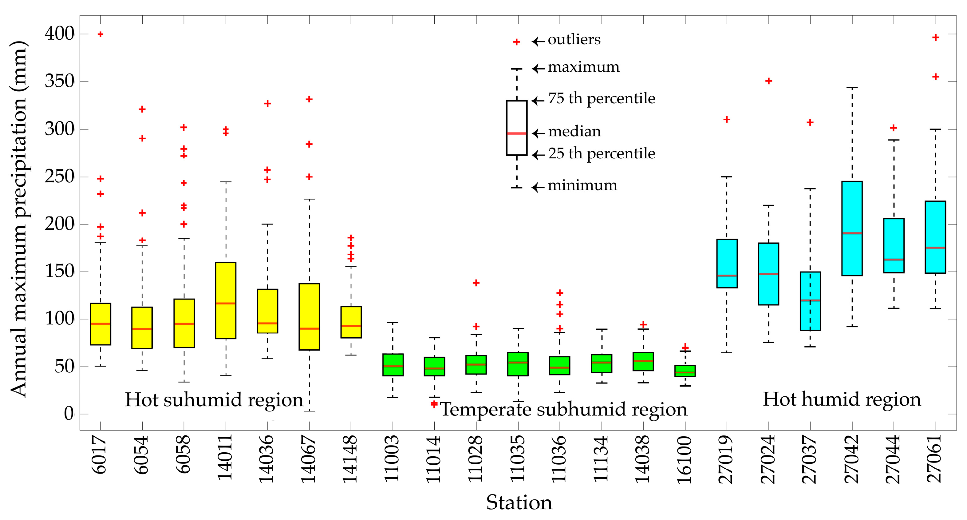
Precipitation in the tropics is higher than in temperate regions, especially in the hot humid region (southeastern Mexico) where it can reach annual values of up to 3000 mm [32], which is reflected in the yearly maximum 24-h precipitation analyzed (Figure 3). Mean values of annual maximum precipitation recorded by the stations in the hot humid region vary between 127 and 200 mm, while in the hot subhumid region they vary from 102 to 126 mm. The temperate subhumid region has lower values, and mean values vary between 46 and 57 mm. As observed in Figure 3, maximum annual precipitations are more variable in the hot region than in the temperate region. The coefficients of variation of the hot subhumid region have large variation, from 31% to 62%, and, in the hot humid region, values are lower, varying from 25% to 37%, while in the temperate subhumid region coefficients of variation vary from 22% to 34%.

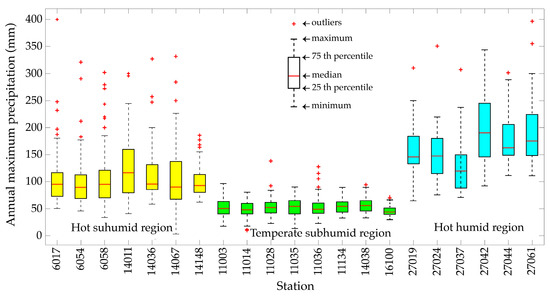
Figure 3. Maximum yearly precipitation recorded at the stations included in the analysis.

3.1. Frequency Analysis

The first step was a frequency analysis to determine which pdf best fit to the series of maximum annual precipitation analyzed. The results show that there is no pdf that adequately represents most of the series analyzed. In general, the LOGGM pdf was the function that most often had the best fit to the series, since in a little more than 40% of the series it was the best fitting pdf, particularly in the series belonging the hot humid region. In addition, in a little more than 20% of the series, it was the second best fitting function. The LP3 pdf, which is of the same family as the LOGGM, was found to have the best fit in almost 20% of the series. If the pdf are considered by family, the pdf most often selected belong to the log-Pearson type 3 family, for a little over 60% of the series. In contrast, the least selected family was the logistic family. A pdf of this family was selected as the best fitting pdf in only 14% of the series. On the other hand, if the pdf are considered by number of parameters, it was observed that two-parameter pdf were selected as the best for 67% of the series, against only 33% of the series in the case of the three-parameter distributions. This is consistent with the BIC tendency towards parsimony, that is, selecting the model with the fewest parameters when the goodness of fit of the models is similar [33].

It is also worth noting that, when the skewness coefficient $\gamma$ was below 0.30, only three-parameter distributions were selected. GLOG or GEV were selected when the $\gamma$ value was slightly negative, but LP3 was selected for the case in which $\gamma =0.29$. In addition, for $\gamma >2$, the LP3 was selected. On the other hand, two-parameter distributions were selected in 15 of the 16 cases in which $0.40<\gamma <1.70$. While GLOG, GEV and LP3 can fit data in this range of $\gamma$ values, the BIC includes a term which penalizes the number of parameters in a distribution, so it will select a two-parameter distribution if it provides a fit similar to that of the best fitting three-parameter distribution. However, for $\gamma <0.30$ and $\gamma >2$, the two-parameter distributions did not provide a sufficiently good fit, so three-parameter distributions were selected instead.

For each of the analyzed series, the best fitting distribution was used as the mother distribution for the generation of the random samples. The best and second best fitting distributions for each of the series are shown in the Table 2.

Table 2. Parameters of the best fitting probability distribution functions.

Name	Best pdf	Second Best pdf	$\mathit{\alpha }$	$\mathit{\beta }$	$\mathit{\theta }$
Madrid	LP3	LOGGM	5.3287144	0.1992481	3.5390657
M. Á. Camacho	LP3	GEV	4.1525277	0.2254003	3.6213723
Tecomán	LOGGM	LLOG	82.634782	0.0555225
Apazulco	LOGGM	GMB	91.842315	0.0514029
Cuautitlán	LP3	GEV	4.376189	0.1731262	3.9173081
Higuera Blanca	GMB	GLOG		51.898719	80.561081
Tecomates	GEV	LP3	0.1945382	19.86305	85.816749
Agua Tibia	LP3	GEV	11.795387	−0.0914924	5.0066864
Cuerámaro	GEV	GLOG	−0.2865803	16.660192	43.524345
Irapuato	LLOG	LOGGM		0.1621175	3.9415775
La Sandía	GLOG	LLOG	0.0823704	9.1261126	54.169179
Adjuntas	LOGGM	LLOG	154.81554	0.0254319
El Conejo	LOGGM	GMB	213.81437	0.0185691
Cuixtla	LOGGM	GMB	286.73673	0.0140327
P. San Isidro	GMB	LOGGM		8.2309395	41.686879
Jalapa	LLOG	LOGGM		0.1493782	5.0432277
La Huasteca	LOGGM	GMB	236.09342	0.0210114
P. Nuevo	LOGGM	LP3	201.45845	0.0237352
Tapijulapa	LOGGM	GMB	235.16545	0.0222989
Teapa	GMB	LOGGM		35.105362	157.71026
Puyacatengo	LOGGM	GMB	313.25914	0.0166501

$\alpha$ is the scale parameter; $\beta$ the shape parameter, and $\theta$ the location parameter.

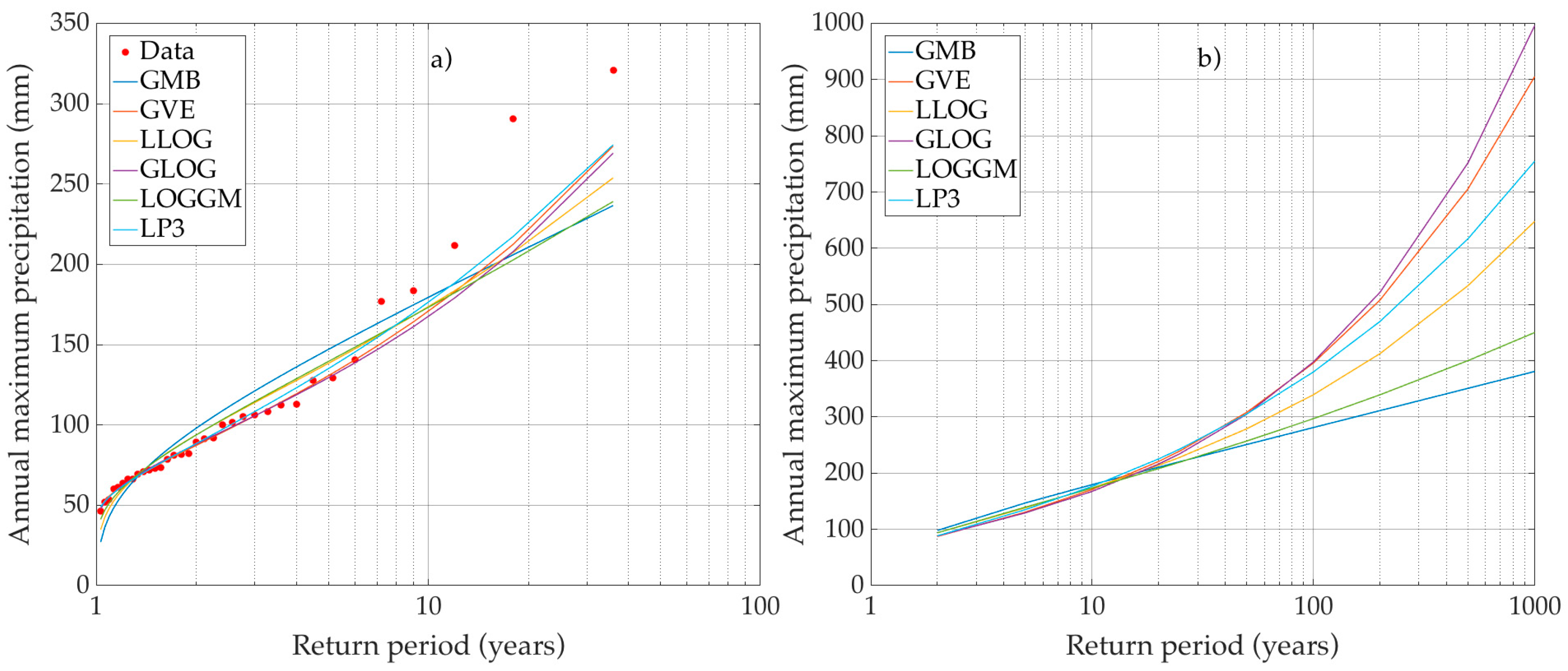
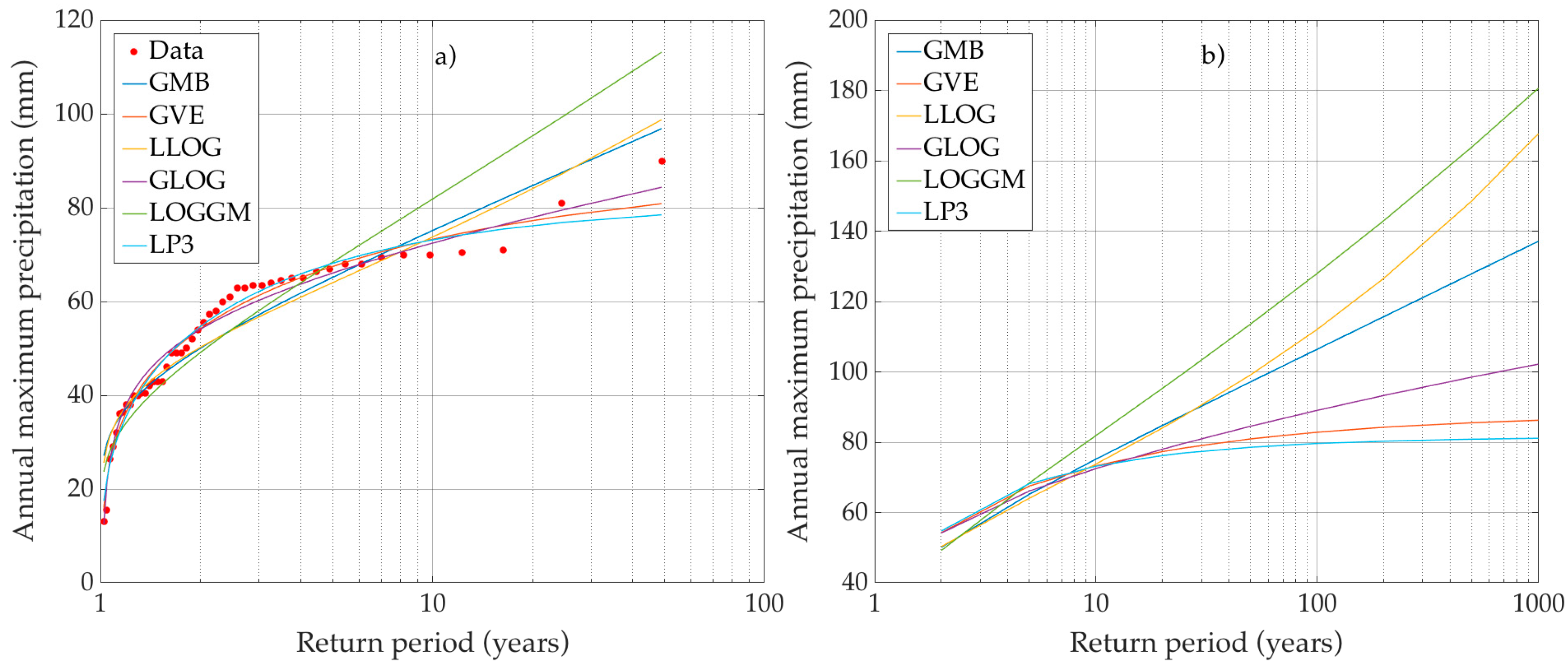
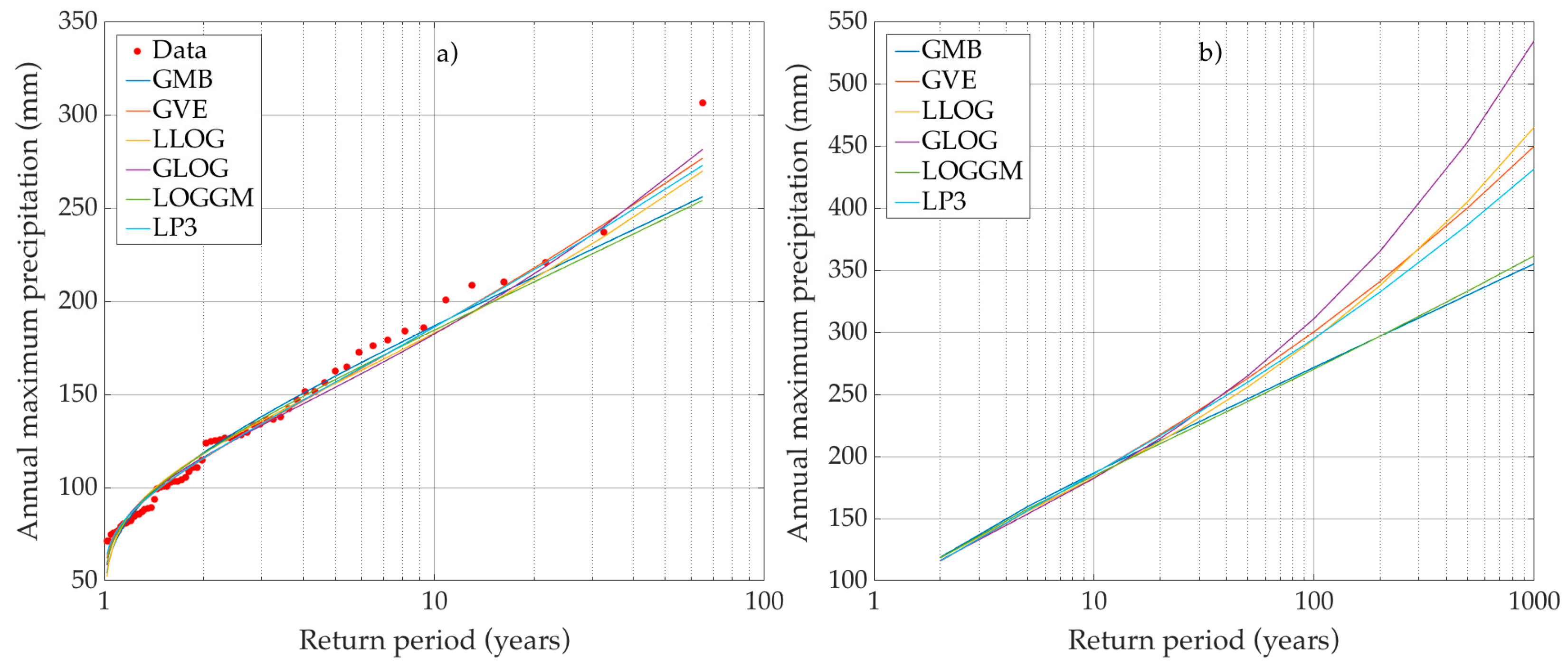
For most of the analyzed series, one or more of the considered distributions provided an adequate fit. Figure 4a, Figure 5a and Figure 6a show the graphs of the fitted distributions for stations 6054, 11035 and 27037. Figure 5a and Figure 6a show examples of adequate fit, whereas Figure 4a provides one of the scarce examples of poor fit. It was observed that for values of $\gamma$ between $0.30$ and $2$, all the distributions provided a similar fit (as in Figure 6a); this means that, the more parsimonious two-parameter distributions were selected by the BIC. However, for values of $\gamma$ above 2 (i.e., Figure 4a), or below 0.30 (i.e., Figure 5a), there were significant differences between the distribution curves, and only three-parameter distributions, if any, provided an adequate fit. The similarities between distribution curves happen mostly within the interpolation region. Outside of this region, differences between curves become grater, increasing with the return period. The distribution curves spread out considerably for return periods with orders of magnitude of 100 and above. This behavior is illustrated in Figure 4b, Figure 5b and Figure 6b, which show the estimated quantiles for stations 6054, 11035 and 27037. It means that for high return periods, the different distributions provide very different estimates of the quantiles. This is true for all the analyzed series, but more so for the high variance and high skew series of the hot subhumid region.

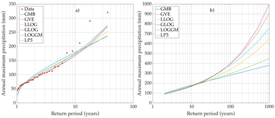
Figure 4. Frequency analysis of maximum yearly precipitation recorded at the station 6054: (a) fitted distributions; and (b) estimated quantiles.

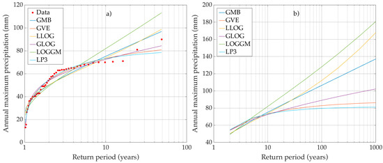
Figure 5. Frequency analysis of maximum yearly precipitation recorded at the station 11035: (a) fitted distributions; and (b) estimated quantiles.

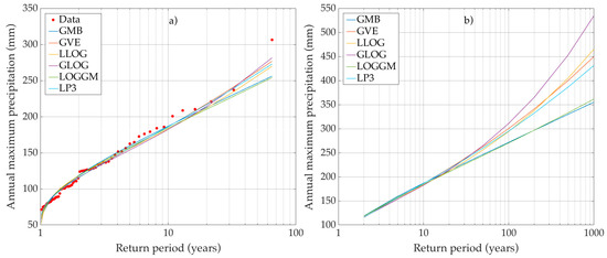
Figure 6. Frequency analysis of maximum yearly precipitation recorded at the station 27037: (a) fitted distributions; and (b) estimated quantiles.

3.2. Construction of Confidence Intervals

Once the best fitting pdf were identified, they were used to estimate the quantiles corresponding to the return periods $T$ = 2, 5, 10, 20, 25, 50, 100, 200, 500 and 1000 years. The confidence intervals were then constructed for those return periods using the four bootstrap techniques.

Because of the large number of intervals obtained, Table 3 gives only those intervals obtained for $T$ = 10, 100 and 1000 years. These intervals show that, for a single series, the intervals increase with respect to the return period and that, in general, the BC and MSB methods give the widest intervals, while BP gives the narrowest intervals. The difference between confidence intervals obtained by the different bootstrap methods is more noticeable when the return periods are longer. In addition, the results indicate that the intervals for the series from the hot humid and hot subhumid regions are wider than those of the series from the temperate subhumid region, since the maximum annual precipitation is more variable (Figure 3).

Table 3. Confidence intervals for the quantiles corresponding to the return periods of 10, 100, and 1000 years.

Station	Climate Region	Fitted pdf	Return Period (Years)	Estimated Quantile (mm)	Confidence Intervals (mm)
					BP	BC	MSB	BCA
6017	Hot subhumid	LP3	10	184	140–237	145–245	146–251	140–256
			100	384	221–720	252–927	240–957	223–1501
			1000	732	300–2166	377–3619	-	314–8071
6054	Hot subhumid	LP3	10	176	133–240	137–250	136–251	133–271
			100	380	206–774	232–947	226–1201	211–1374
			1000	755	282–2487	351–5165	-	315–9317
6058	Hot subhumid	LOGGM	10	191	155–233	157–238	158–240	155–243
			100	358	242–543	253–574	254–606	244–608
			1000	590	321–1191	345–1328	353–1796	329–1424
14011	Hot subhumid	LOGGM	10	213	175–259	177–262	176–263	175–266
			100	381	283–512	288–521	287–528	281–536
			1000	596	408–887	417–903	416–926	405–920
14036	Hot subhumid	LP3	10	174	145–210	149–218	147–214	145–225
			100	317	213–522	229–642	220–570	215–789
			1000	541	285–1325	323–2169	307–2285	296–2941
14067	Hot subhumid	GMB	10	197	164–237	166–240	165–240	163–247
			100	319	260–392	262–394	262–398	253–411
			1000	439	352–543	357–550	356–555	344–572
14148	Hot subhumid	GEV	10	142	122–166	124–172	123–168	123–174
			100	234	163–365	171–404	166–392	165–436
			1000	375	194–901	211–1095	211–1695	206–1241
11003	Temperate subhumid	LP3	10	74.1	68.0–80.5	68.1–80.5	68.4–80.8	67.7–81.3
			100	92.1	79.4–108	76.8–105	80.0–109	78.0–105
			1000	104	83.1–136	77.8–129	84.1–137	81.8–126
11014	Temperate subhumid	GEV	10	71.2	64.7–77.0	65.1–77.4	65.3–78.1	64.6–77.6
			100	86.1	74.5–100	74.1–99.2	75.2–101	73.6–100
			1000	93.6	77.4–120	77.0–119	77.1–119	77.3–119
11028	Temperate subhumid	LLOG	10	73.5	67.1–81.1	67.6–82.3	67.1–81.0	66.5–84.1
			100	108	93.2–128	94.9–132	93.3–128	92.3–137
			1000	158	127–200	131–208	128–200	126–222
11035	Temperate subhumid	GLOG	10	72.5	66.7–78.1	67.1–78.4	67.2–78.7	65.9–79.6
			100	89.1	78.0–104	78.1–104	78.0–104	76.0–108
			1000	102	83.9–134	84.1–135	83.2–133	82.0–140
11036	Temperate subhumid	LOGGM	10	77.3	69.4–86.1	69.5–86.4	69.6–86.4	68.8–87.4
			100	111	94.5–131	95.4–132	95.0–132	93.7–135
			1000	147	119–181	121–185	120–183	117–190
11134	Temperate subhumid	LOGGM	10	75.3	66.1–85.9	66.7–86.8	66.4–86.2	65.9–87.8
			100	102	83.7–125	84.7–127	84.9–126	83.2–131
			1000	129	100–168	101–171	102–170	98.6–175
14038	Temperate subhumid	LOGGM	10	76.0	69.6–83.0	69.9–83.3	69.7–83.3	69.4–84.3
			100	99.2	87.0–113	87.5–114	87.3–114	86.5–115
			1000	121	103–144	104–145	103–145	102–147
16100	Temperate subhumid	GMB	10	60.2	54.3–66.7	54.3–66.8	54.5–66.9	53.9–67.6
			100	79.6	69.3–91.8	69.4–92.0	69.5–92.0	68.4–92.9
			1000	98.5	83.7–116	84.0–117	84.1–117	82.5–118
27019	Hot humid	LLOG	10	215	191–246	193–247	190–245	190–254
			100	308	253–386	258–392	252–384	251–411
			1000	435	329–602	339–610	329–600	325–665
27024	Hot humid	LOGGM	10	217	186–253	185–252	187–255	180–264
			100	312	248–395	249–395	250–399	236–425
			1000	411	307–559	308–564	311–569	289–618
27037	Hot humid	LOGGM	10	185	164–208	164–208	165–208	162–212
			100	270	226–322	229–327	229–325	224–340
			1000	362	289–453	293–465	292–460	284–488
27042	Hot humid	LOGGM	10	295	257–337	258–338	259–339	257–342
			100	434	355–531	358–542	359–534	355–544
			1000	581	450–758	457–771	457–764	452–782
27044	Hot humid	GMB	10	237	214–263	215–265	214–263	214–269
			100	319	279–368	280–371	279–368	277–376
			1000	400	342–472	344–475	343–473	338–483
27061	Hot humid	LOGGM	10	270	234–305	235–307	237–309	230–312
			100	375	305–450	308–456	311–461	298–470
			1000	480	370–611	374–619	378–629	363–652

The blank cells indicate cases in which negative values were obtained for the upper limit. This anomaly occurred only with the MSB confidence intervals, for the return periods of 500 or 1000 years, indicating a defect in this method. In the methodology section, we mentioned that to calculate the upper limit of the confidence interval of a quantile ${\widehat{x}}_T$ of a three-parameter distribution with the MSB method, the difference $UI=\frac{1}{{\widehat{x}}_T}-\left({\mathrm{z}}_{1-\frac{\alpha }{2}}\right){\sigma }_{uT}$ must be calculated. This difference was negative in some cases, and, therefore, the upper limit $XS=1/UI$ was also negative, which is an unacceptable result. Thus, the MSB method does not function in some cases and its use is not recommended.

It was observed that the size of the confidence intervals was related to both the standard deviation $\sigma$ and the skewness coefficient $\gamma$ of the series. The five series with the widest confidence intervals were Manuel Ávila Camacho (6054), Madrid (6017), Cuautitlán (14036), Tecomán (6058) and Tecomates (14148). All five belong to the hot subhumid region, where the estimated values of $\sigma$ were relatively high. On the other hand, the series from the temperate subhumid region had the smallest estimates of $\sigma$ and therefore, the narrowest confidence intervals. The three series with the widest intervals (6054, 6017 and 14036) also had the highest estimated values of $\gamma$. A relationship between the size of the intervals and the best fitting pdf was also observed. Of the five series with the widest intervals, the best fitting pdf had three parameters in four of the cases. For the three series with the widest confidence intervals, the best fitting pdf was the LP3.

3.3. Comparison of Bootstrap Techniques

As we pointed out earlier, the best fitting pdf were used as mother distributions to generate random samples and, for each of the mother distributions, two or three different scenarios were considered.

Considering the combination of all the mother distributions, possible scenarios, bootstrap techniques and return periods, the number of coverage values obtained was very large. Table 4 shows a summary of the obtained results. Only the maximum, minimum and average of all the coverages for each time series and return periods analyzed are shown. According to the selected confidence level of 95%, the minimum, maximum and average coverage should be 95%. In practice, we consider the coverage to be adequate if the maximum coverage is not far above 95%, the minimum coverage is not far below, and the average coverage is around 95%.

Table 4. Coverages obtained for different mother distributions and fitted pdf.

Station	Mother Distribution	Fitted pdf	Coverage (%)
			BP			BC			MSB			BCA
			Max	Min	Mean	Max	Min	Mean	Max	Min	Mean	Max	Min	Mean
6017	LP3, $\alpha =5.33$, $\beta =0.199$, $\theta =3.54$	LP3	94	89	90	93	90	91	93	51	83	96	93	95
		LOGGM	92	44	71	91	48	73	91	50	73	92	57	79
6054	LP3, $\alpha =4.15$, $\beta =0.225$, $\theta =3.62$	LP3	95	86	88	94	89	90	94	38	78	94	93	93
		GEV	94	90	91	93	89	91	92	21	75	94	93	93
		LOGGM	90	40	67	89	44	69	89	46	69	91	54	76
6058	LOGGM, $\alpha =82.6$, $\beta =0.0555$	LOGGM	95	93	94	95	93	94	95	94	93	96	95	93
		LLOG	98	91	96	98	83	94	98	90	95	99	90	97
		LP3	94	92	93	95	91	93	95	90	94	96	93	95
11003	LP3, $\alpha =11.8$, $\beta =-0.091$, $\theta =5.01$	LP3	97	94	96	95	92	93	97	95	96	96	92	94
		GEV	95	94	94	95	93	94	95	94	94	96	94	95
		LOGGM	99	8	63	99	7	60	99	8	61	99	11	64
11014	GEV, $\alpha =-0.287$, $\beta =16.7$, $\theta =43.5$	GEV	95	93	93	95	91	93	95	92	93	96	94	94
		GLOG	99	90	95	99	84	94	99	85	95	100	88	96
		GMB	100	1	59	99	0	57	99	0	58	100	1	60
11028	LOGL, $\beta =0.162$, $\theta =3.94$	LOGL	95	95	95	95	94	94	95	95	95	97	95	97
		LOGGM	94	54	84	94	57	84	94	56	84	96	64	88
		GLOG	95	94	94	95	93	94	95	93	94	97	95	96
11035	GLOG, $\alpha =0.0824$, $\beta =9.13$, $\theta =54.2$	GLOG	95	93	94	94	92	93	94	93	93	96	93	94
		LLOG	100	2	59	100	1	55	100	2	60	100	2	59
11036	LOGGM, $\alpha =155$, $\beta =0.0254$	LOGGM	95	94	94	95	94	95	95	94	94	97	94	96
		LLOG	98	81	93	98	74	92	98	81	93	99	82	95
		LP3	95	92	93	94	92	93	94	93	94	96	94	95
11134	LOGGM, $\alpha =214$, $\beta =0.0186$	LOGGM	94	94	94	95	94	94	94	94	94	97	94	96
		GMB	97	94	96	97	95	96	97	94	96	99	95	98
		LP3	95	92	93	94	90	92	95	93	94	95	93	94
14011	LOGGM, $\alpha =91.8$, $\beta =0.0514$	LOGGM	95	93	94	94	93	94	94	93	94	96	93	96
		GMB	93	23	67	92	25	68	91	27	69	94	33	75
		LP3	95	92	94	94	92	93	95	90	94	96	94	95
14036	LP3, $\alpha =4.38$, $\beta =0.173$, $\theta =3.92$	LP3	95	90	91	94	92	93	95	81	91	96	95	95
		GEV	94	91	92	94	91	92	93	61	87	95	94	95
		LOGGM	86	25	60	86	28	62	86	28	62	90	35	68
14038	LOGGM, $\alpha =286$, $\beta =0.0140$	LOGGM	95	93	94	96	93	94	95	93	94	97	96	96
		GMB	97	92	95	97	90	94	97	90	94	98	94	97
		LP3	94	93	93	95	92	93	94	93	94	96	94	95
14067	GMB, $\beta =51.9$, $\theta =80.6$	GMB	95	93	94	95	94	94	95	94	94	97	95	95
		GLOG	99	91	96	97	93	95	97	91	95	99	93	97
		GEV	95	89	91	95	89	91	94	90	92	95	92	93
14148	GEV, $\alpha =0.195$, $\beta =19.9$, $\theta =85.8$	GEV	92	87	89	92	86	88	92	66	86	94	90	92
		LP3	95	82	87	92	85	88	94	76	86	94	91	93
		GMB	90	8	57	88	9	57	88	9	57	91	14	64
16100	GMB, $\beta =8.23$, $\theta =41.7$	GMB	94	94	94	94	94	94	94	94	94	97	95	96
		LOGGM	94	78	87	94	82	88	94	80	87	96	87	92
		GEV	94	91	92	94	91	92	94	91	92	95	93	94
27019	LLOG, $\beta =0.149$, $\theta =5.04$	LLOG	95	94	95	95	94	94	96	94	94	97	94	97
		LOGGM	94	63	86	94	67	86	94	66	86	97	73	90
		GLOG	95	93	93	95	92	92	95	90	93	96	95	95
27024	LOGGM, $\alpha =236$, $\beta =0.0210$	LOGGM	96	95	95	96	95	95	96	95	95	98	95	97
		GMB	94	92	93	95	93	94	94	93	93	97	94	96
		LP3	95	93	93	94	91	92	94	93	94	96	93	94
27037	LOGGM, $\alpha =201$, $\beta =0.0237$	LOGGM	95	93	93	95	93	94	95	93	94	96	95	96
		LP3	94	93	93	94	91	92	94	93	94	95	94	95
27042	LOGGM, $\alpha =235$, $\beta =0.0223$	LOGGM	95	93	94	96	93	95	96	94	95	97	94	96
		GMB	95	89	93	94	90	93	95	91	93	97	94	96
		LP3	95	92	93	94	90	92	95	93	94	96	93	94
27044	GMB, $\beta =35.1$, $\theta =158$	GMB	96	94	95	95	94	95	95	94	95	97	95	97
		LOGGM	94	82	88	95	85	89	94	84	89	96	89	92
		GEV	95	93	93	95	92	93	95	93	93	96	95	95
27061	LOGGM, $\alpha =313$, $\beta =0.0167$	LOGGM	95	94	94	95	94	94	95	94	94	97	94	96
		GMB	96	94	95	96	94	95	96	94	95	98	94	97
		LP3	94	92	93	94	90	92	94	93	93	96	93	94

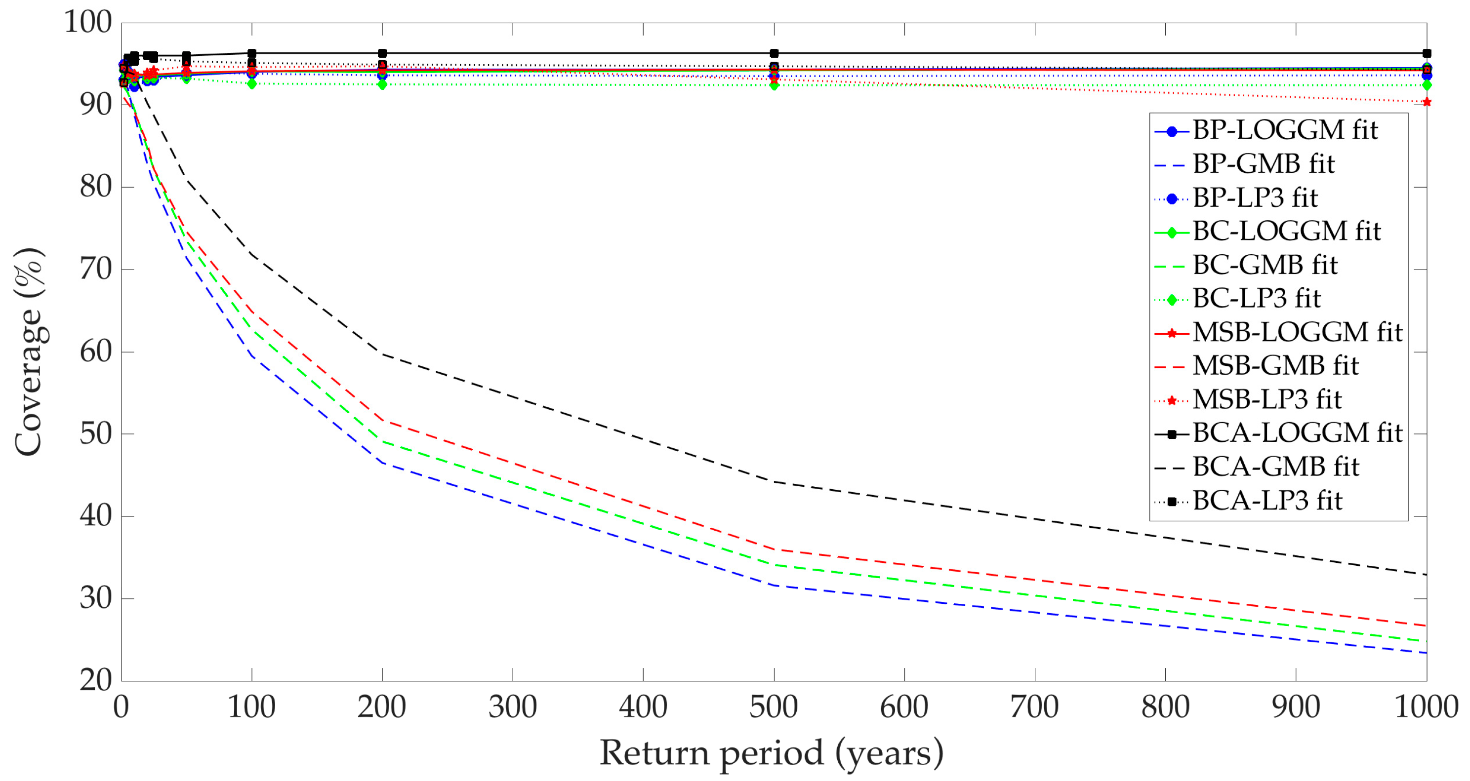
As an example, Figure 7 shows the coverages obtained for the resulting mother distribution in the series of the Apazulco station (14011). Each of the curves corresponds to the combination of a fitted pdf and a bootstrap technique. Thus, the curve with the legend “BP—LOGGM fit” corresponds to a coverage obtained when the pdf used for the fit was LOGGM, and the technique used to construct the confidence intervals was BP. Each bootstrap technique is distinguished by a different color. The fit by the LOGGM pdf (which coincides with the mother pdf) is seen as continuous lines, the fit by the GMB pdf by broken lines, and the fit by the LP3 pdf by dotted lines. In the figure, it can be seen that when the fitted pdf is LOGGM, the coverage obtained is good for the four bootstrap techniques since it takes values near 95% for all of the return periods. Coverage is also good when the fitted pdf is LP3 since it never falls below 90%. In contrast, when the fitted pdf is GMB, the coverage of the bootstrap intervals is not adequate since it falls below 90% for $T\ge 20$, and below 60% for $T\ge 200$. In Table 4, it can be seen that, when LOGGM and LP3 pdf are fitted, the maximum and average coverages always remain near 95%, while the minimum coverage never falls below 90%. However, for the GMB pdf, average coverage is always less than 80% and the minimum is always below 35%.

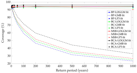
Figure 7. Coverages for the Apazulco station (14011) for a LOGGM mother distribution.

The results indicate that the BCA coverages were almost always higher than those obtained with the other techniques. It was observed that the BP coverage was very similar to that of the BC. It was also found that in scenarios corresponding to the mother distributions taken from the series Madrid (6017) and Manuel Ávila Camacho (6054) the MSB technique failed, while BP and BC performed well. This is due to the defect pointed out above that when a negative value is obtained for the upper limit, the quantile value is outside the confidence interval.

In those scenarios in which the fitted pdf was equal to the mother pdf, the coverages were generally good. When the mother distribution had three parameters, the BCA intervals had the coverage closest to the 95% confidence level. This is because the wider BCA intervals are more likely to contain the true values of the larger quantiles estimated for the three parameters distributions. On the other hand, when the mother distribution had two parameters, all techniques performed similarly well.

For the scenarios in which a pdf different from the mother pdf was fitted, coverage was always good when the fitted pdf had three parameters ($\ge$90%). When the fitted pdf had two parameters, coverage was not always poor, however, when coverage was poor (<60%), the fitted pdf had two parameters. This makes sense since, when there was great variability, the confidence intervals for three-parameter distribution quantiles were generally wider than for two-parameter distribution quantiles. Thus, the confidence intervals for the three-parameter distribution quantiles were wide enough that it was highly probable that they contained the quantiles of the mother distribution. The same was not always true for the confidence intervals for two-parameter distributions. It may be assumed that it is convenient to always use three-parameter distributions, because that would assure that the confidence intervals have adequate coverage. However, there is more uncertainty in the estimation of the quantiles of a three-parameter distribution, which would affect decision-making.

On the other hand, the BIC selects a distribution following two criteria: the degree of fit and the number of parameters. According to the law of parsimony, the BIC will select the simplest model (the model with the least parameters) that adequately fits the data. Therefore, when it selects a three-parameter distribution instead of a two-parameter distribution, it does so necessarily because of its better fit. Surely, the two-parameter distribution could not approximate well the form of the distribution of the data, while the three-parameter distribution, which can adopt a larger variety of forms, could. However, if several two-parameter distributions are considered as hypothetical distributions, it is possible that together they can adopt the variety of forms that the three-parameter distribution can take, and that one of them could fit well the analyzed series. This distribution would be selected, avoiding the higher level of estimation uncertainty associated with the use of three-parameter distributions.

4. Conclusions

No single distribution provided the best fit always. Two-parameter distributions were selected more frequently than those of three parameters by the BIC. However, in cases in which the coefficient of skew was below 0.30, or when it was greater than 2.00, the two-parameter distributions did not provide a good fit, so three-parameter distributions were selected.

In some cases, there were considerable differences in the tails of the fitted distributions, which resulted in vastly different estimates of the quantiles for large return periods. Both two- and three-parameter distributions should be considered for frequency analysis of hydrological extremes, and an adequate selection criterion should be used to select the best fitting distribution. The advantage of two-parameter distributions is that there is less uncertainty in the estimation of the quantiles, which results in narrower confidence intervals. However, there will be cases in which two-parameter distributions will not provide adequate fit. Three-parameter distributions provide a good fit for a wider variety of cases than two-parameter distributions, so they should be considered for those cases in which the later do not provide an adequate fit. Whenever both two- and three-parameter distributions provide an adequate fit, the two-parameter distribution should be selected, since the estimation uncertainty is lower.

We recommend that log-gamma, which is seldom used in hydrology, should be considered among the two-parameter distributions used for frequency analysis of hydrological extremes. In this study, it was the most frequently selected distribution (9 of the 21 series analyzed), outperforming the Gumbel and GEV distributions, which are used in Mexico for analysis of annual maximum precipitations.

The confidence intervals obtained in this study with bootstrap techniques had adequate coverage in cases in which the fitted pdf was correct. In addition, when the fitted pdf was incorrect but had three parameters, the coverage was adequate when that distribution was either the second best fitting or of the same family as a best fitting two parameter distribution. In contrast, in all cases in which the four techniques performed poorly, an incorrect two-parameter pdf was fit, and it did not provide an adequate fit. Therefore, the quantiles estimated from the two-parameter distributions were very different from the quantiles of the mother distribution, and the confidence intervals were not wide enough to include these quantiles with a high probability. This confirms the need of an adequate criterion for selecting the distribution for frequency analysis. If an inappropriate distribution is chosen, not only the quantiles will be incorrectly estimated, but the confidence intervals will give a false idea of the estimation uncertainty.

In general, the widest confidence intervals were obtained with the BCA and MSB techniques, while the narrowest were obtained with the BP technique. When the fitted pdf has three parameters the use of BCA is recommended. On the other hand, it was observed that when the fitted pdf was correct and had two parameters, the BP, BC and BCA techniques had similar performance. Therefore, when the fitted pdf has two parameters, it is recommended to use the BP technique, since it gives narrower intervals and is easier to program. The MSB technique is not recommended because it failed in situations in which the other techniques had better results.

References

- Botto, A.; Ganora, D.; Laio, F.; Claps, P. Uncertainty compliant design flood estimation. Water Resour. Res. 2014, 50, 4242–4253. [Google Scholar] [CrossRef]
- Di Baldasarre, G.; Laio, F.; Montanari, A. Effect of observation errors on the uncertainty of design floods. Phys. Chem. Earth 2011, 42–44, 85–90. [Google Scholar] [CrossRef]
- Hall, M.J.; Van den Boogaard, H.F.P.; Fernando, R.C.; Mynett, A.E. The construction of confidence intervals for frequency analysis using resampling techniques. Hydrol. Earth Syst. Sci. 2004, 8, 235–246. [Google Scholar] [CrossRef]
- Flowers Cano, R.S.; Flowers Robert, J.; Rivera-Trejo, F. Evaluación de criterios de selección de modelos probabilísticos: Validación con series de valores máximos simulados. Tecnol. Cienc. Agua 2014, 5, 189–197. [Google Scholar]
- Cheng, K.-S.; Chiang, J.-L.; Hsu, C.-W. Simulation of probability distributions commonly used in hydrological frequency analysis. Hydrol. Process. 2007, 2, 51–60. [Google Scholar] [CrossRef]
- Silva, A.T.; Naghettini, M.; Portela, M.M. Sobre a estimacao de intervalos de confianca para os quantis de variáveis aleatórias hidrológicas. Recur. Hidr. 2011, 32, 63–76. [Google Scholar] [CrossRef]
- Liu, Y.; Gupta, H.V. Uncertainty in hydrological modeling: Toward an integrated assimilation framework. Water Resour. Res. 2007, 43, W07401. [Google Scholar] [CrossRef]
- Carpenter, J.; Bithell, J. Bootstrap confidence intervals: When, which, what? A practical guide for medical statisticians. Stat. Med. 2000, 19, 1141–1164. [Google Scholar] [PubMed]
- Helsel, D.R.; Hirsch, R.M. Statistical Methods in Water Resources, 1st ed.; Elsevier Science Publishers: Amsterdam, The Netherlands, 1992; 522p, ISBN 0-444-88528-5. [Google Scholar]
- DiCiccio, T.J.; Efron, B. Bootstrap confidence intervals. Stat. Sci. 1996, 11, 189–228. [Google Scholar]
- Davison, A.C.; Hinkley, D.V. Bootstrap Methods and Their Application, 1st ed.; Cambridge University Press: Cambridge, UK, 1997; p. 594. ISBN 978-0-521-57391-7. [Google Scholar]
- Efron, B. Bootstrap methods: Another look at the jackknife. Ann. Stat. 1979, 7, 1–26. [Google Scholar] [CrossRef]
- Kyselý, J. A cautionary note on the use of nonparametric bootstrap for estimating uncertainties in extreme-value models. J. Appl. Meteorol. Climatol. 2008, 42, 3236–3251. [Google Scholar] [CrossRef]
- Efron, B.; Tibshirani, R. Bootstrap methods for standard errors, confidence intervals, and other measures of statistical accuracy. Stat. Sci. 1986, 1, 54–75. [Google Scholar] [CrossRef]
- Kyselý, J. Coverage probability of bootstrap confidence intervals in heavy tailed frequency models, with application to precipitation data. Theor. Appl. Climatol. 2010, 101, 345–361. [Google Scholar] [CrossRef]
- Liu, B.H. Statistical Genomics. Linkeage, Mapping and QTL Analysis, 1st ed.; CRC Press: Boca Raton, FL, USA, 1997; p. 648. ISBN 0849331668. [Google Scholar]
- Lee, S.M.S. Nonparametric confidence intervals based on extreme bootstrap percentiles. Stat. Sin. 2000, 10, 475–496. [Google Scholar]
- Hernández-Abreu, E.; Martínez-Pérez, M. El método bootstrap en la estimación de incertidumbres. BCT INIMET 2012, 1, 8–16. [Google Scholar]
- Correa, J.C.; Sierra, E. Intervalos de confianza para la comparación de dos proporciones. Rev. Colomb. Estad. 2003, 26, 61–75. [Google Scholar]
- Van de Boogaard, H.F.P.; Hall, M.J. The construction of confidence intervals for frequency analysis using resampling techniques: A supplementary note. Hydrol. Earth Syst. Sci. 2004, 8, 1174–1178. [Google Scholar] [CrossRef]
- Comisión Nacional del Agua (CONAGUA). Base de Datos en el Sistema CLIma COMputarizado (CLICOM); Servicio Meteorológico Nacional, Comisión Nacional del Agua: Mexico, Mexico, 2016; (In Spanish). Available online: http://smn.cna.gob.mx/index.php?option=com_content&view=article&id=42&Itemid=75 (accessed on 17 January 2016).
- Efron, B. Censored data and the bootstrap. J. Am. Stat. Assoc. 1981, 76, 312–319. [Google Scholar] [CrossRef]
- Eakin, B.K.; McMillen, D.P.; Buono, M.J. Constructing confidence intervals using the bootstrap: An application to a multi-product cost function. Rev. Econ. Stat. 1990, 72, 339–344. [Google Scholar] [CrossRef]
- Efron, B. Non-Parametric Standard Errors and Confidence Intervals. Available online: https://statistics.stanford.edu/sites/default/files/BIO%2067.pdf (accessed on 15 December 2017).
- Efron, B. The Jackknife, the Bootstrap and Other Resampling Plans; CBMS-NSF Regional Conference Series in Applied Mathematics, Monograph 38; Society for Industrial and Applied Mathematics: Philadelphia, PA, USA, 1982; p. 92. ISBN 9780898711790. [Google Scholar]
- Efron, B. Better Bootstrap Confidence Intervals. Available online: http://oai.dtic.mil/oai/oai?verb=getRecord&metadataPrefix=html&identifier=ADA150798 (accessed on 15 December 2017).
- Efron, B. Transformation theory: How normal is a one parameter family of distributions? Ann. Stat. 1982, 10, 323–339. [Google Scholar] [CrossRef]
- Neter, J.; Wasserman, W. Applied Linear Statistical Models: Regression, Analysis of Variance, and Experimental Designs, 6th ed.; Richard, D., Ed.; Irwin, Inc.: Homewood, IL, USA, 1976; p. 842. ISBN 0256014981. [Google Scholar]
- Nguyen, V.T.V.; Nguyen, T.H. Statistical modeling of extreme rainfall processes (SMExRain): A decision support tool for extreme rainfall frequency analyses. Procedia Eng. 2016, 154, 624–630. [Google Scholar] [CrossRef]
- Schwarz, G. Estimating the dimension of a model. Ann. Stat. 1978, 6, 461–464. [Google Scholar] [CrossRef]
- DiDonato, A.R.; Morris, A.H. Computation of the incomplete gamma function ratios and their inverse. ACM Trans. Math. Softw. 1986, 12, 377–393. [Google Scholar] [CrossRef]
- Instituto Nacional de Ecología-Secretaría de Medio Ambiente y Recursos Naturales (INE-SEMARNAT). Cuarta Comunicación Nacional ante la Convención Marco de las Naciones Unidas sobre el Cambio Climático, 1st ed.; Instituto Nacional de Ecología: Mexico, Mexico, 2010; p. 273. ISBN 978-607-7908-00-5. (In Spanish)
- Laio, F.; Di Baldasarre, G.; Montanari, A. Model selection techniques for the frequency analysis of hydrological extremes. Water Resour. Res. 2009, 45, W07416. [Google Scholar] [CrossRef]
© 2018 by the authors. Licensee MDPI, Basel, Switzerland. This article is an open access article distributed under the terms and conditions of the Creative Commons Attribution (CC BY) license (http://creativecommons.org/licenses/by/4.0/).