Abstract
The solar terminator, due to its unique characteristics, is a remarkable source of atmospheric disturbances. Due to its regularity and constancy, dependent solely on geometric factors, it can serve as a test source of disturbances, which can be used to test the response of the medium through which it passes and determine its state. However, our knowledge of the atmospheric phenomena generated by the terminator is far from complete. One clear indication of the terminator’s influence is geomagnetic disturbances manifested in the vertical and eastward components of the magnetic field measured at magnetic observatories. To determine the sources of geomagnetic disturbances from the solar terminator, which can be identified by the strict phase correlation of these disturbances with the moments of terminator passage, ionospheric irregularities arising during terminator passage were studied. Ionospheric irregularities extending along the boundary of the morning solar terminator were detected in total electron content data, based on measurements by GNSS receivers. Assumptions are made about the possible parameters of the ionospheric current structure that creates variations in the magnetic field associated with the passage of the solar terminator.
1. Introduction
As recent studies have shown [1], the Earth’s magnetic field data measured at geomagnetic observatories contain distinct, very weak disturbances, precisely time-locked to the passage of the solar terminator at the magnetic observatory point, as well as to the passage of the terminator at its magnetically conjugate point. These magnetic field variations, which we will refer to as St (Solar Terminator) variations by analogy with other types of geomagnetic variations, are detected in the vertical Z component of the magnetic field for all mid-latitude observatories (at least up to 50° latitude). They are highly synchronous oscillations consisting of 1–2 oscillation periods with relatively small average amplitudes of about 1 nT or less. The main feature of these St variations, distinguishing them from other known variations and pulsations, is the precise timing of observations relative to the moments of solar terminator passage, with an accuracy of up to several minutes.
Regular variations in the magnetic field, such as Sq (Solar quiet variations—a variation in the geomagnetic field that depends primarily on local solar time and is observed in the absence of disturbances caused by the solar wind [2]), are created by ionospheric and magnetospheric currents [2,3,4]. Most likely, the considered in this paper St variations in the magnetic field are created by ionospheric currents, just like Sq variations. The short duration of these variations and their clear time reference indicate certain features of the ionospheric currents that create them and their differences from, say, Sq current structures. Synchronicity with the moments of the terminator suggests that the ionospheric current should flow along the terminator line, at least at mid-latitudes. The short duration and rapid change in St variations suggest that the current structure should be quite narrow, on the order of hundreds of kilometers or less, which distinguishes it from the Sq current structure, which extends throughout the daytime side of the ionosphere [2,3].
This paper examines the ionospheric current structures responsible for the magnetic field variations associated with the passage of the solar terminator (St variations).
Investigating these variations for all latitudes and for the morning and evening terminators, as well as magnetically conjugate terminators, is currently too large a task. In this work, we were able to identify a structure in the ionosphere associated with the passage of the morning terminator in the mid-latitudes of the Northern Hemisphere.
2. Data
The work is based on data from measurements of the Earth’s magnetic field, carried out at geomagnetic observatories of the IAGA standard and provided by the INTERMAGNET (International Real-time Magnetic Observatory Network) network [5], as well as data from measurements of the total electron content of the ionosphere, carried out on the basis of data from permanent GNSS receivers.
Data from permanent GNSS receivers (Continuously Operating Reference Station, CORS) located across the continental United States and provided by NOAA NGS (National Oceanic and Atmospheric Administration’s National Geodetic Survey, USA) were used. All observation files in RINEX format were downloaded from the website https://geodesy.noaa.gov/corsdata/rinex/ (accessed on 16 October 2025). The NOAA CORS network was chosen due to its extensive coverage, high and relatively uniform station density across mid-latitudes, and easy data access.
The study used data from all receivers located in the region [30–50° N; 80–120° W], which includes about 1500 receivers. All further calculations of the total electron content (TEC) of ionosphere were performed based on observational RINEX files versions 2 and 3. RINEX (Receiver Independent Exchange Format) is a standardized text-based file format designed for the exchange of Global Navigation Satellite System (GNSS) data, such as GPS, GLONASS, and Galileo [IGS formats and standards, https://www.igs.org/formats-and-standards/ (accessed on 16 October 2025)]. The TEC values were calculated for all receivers using the methodology described in [6,7]. Frequencies L1/L2 for the GPS and GLONASS systems and L1/L5 for the GALILEO system were used with the corresponding frequency coefficients. For further calculations, we used all satellite-to-receiver tracks with an elevation angle greater than 15°. Thus, for each GNSS receiver, TEC values were obtained on average at three dozen ionospheric points, calculated for the approximate height of the maximum ionospheric concentration, 300 km. The calculated TEC values, regardless of the initial time resolution of the RINEX files, in most cases equal to 15 or fewer seconds, were averaged to a one-minute time resolution. Long-period harmonics with periods longer than 20 min and 60 min were removed from these one-minute TEC time series, and the TEC variation values for each ionospheric point were then gridded on a uniform grid with a 0.25° step in latitude and longitude. Thus, maps of TEC variations were constructed for the region [30–50° N; 80–120° W], with a temporal resolution of 1 min (the same procedure is described in more detail in [8]). In total, we processed 340 days from 2023–2024, distributed approximately evenly across the seasons. These maps for the days for which the analysis was conducted are posted on the project website [http://geomag.ionos.kz/tec_project/ (accessed on 16 October 2025)].
3. Method
Despite the fact that the solar terminator itself, and, in particular, the shock wave it generated in the atmosphere, are a very weak source of disturbances [9,10,11,12], and the observed primary effects from it are usually lost against the background of daily disturbances, the clear synchronicity of these effects with the moments of sunrise and sunset make it possible to successfully detect these effects using the method of epoch superposing [1,11].
Since the time and location of the solar terminator’s passage across the planet’s surface are determined solely by the geometry of the planet’s spin around its own axis and orbital rotation [13,14,15], this source of disturbances can be considered highly regular. And since the terminator, that is, the boundary of solar illumination change, moves across the entire planet, on certain scales the terminator can be considered as extended source [12], and therefore possessing (at least on certain scales, at least 10–20 degrees latitude) the corresponding symmetry. Accordingly, the primary effects generated by the terminator’s passage should exhibit coherence in both the temporal and spatial domains. This is the basis for the epoch superposition method used in this study.
Figure 1A shows St variations in the vertical Z component of the geomagnetic field measured on 2000–2025 at the BOU Observatory, Boulder, CO, USA. The diagram is constructed by averaging values for each minute and each day of year of 1 min Z component measurement data for which periods longer than 1 h have been removed [1]. As can be seen, the magnetic measurement data contain clear St variations in the magnetic field at the moments of passage of the morning and evening solar terminators (disturbances along the solid lines in the figure), and a disturbance at the moment of passage of the terminator at the magnetically conjugate point of the observatory (disturbance along the dotted line) is also clearly visible. Figure 1B shows the monthly average time series calculated relative to the moment of the morning and evening solar terminators. This diagram is constructed due to the coherence property of the primary disturbances from the solar terminator in the time domain.
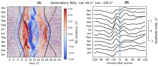
Figure 1.
Variations in the vertical Z component of the magnetic field with periods less than 1 h, averaged over 2000–2024 for BOU observatory. (A) Solid black lines show the moments of passage of the morning and evening solar terminator at ground level of the observatory point. The gray solid lines show the range of +/−2 h from the terminator demonstrated on panel B. Dashed lines show the moments of passage of the morning and evening solar terminator at the magnetically conjugate point. (B) Monthly averaged time series calculated relative to the moment of the morning solar terminator.
The disturbance pattern shown in Figure 1 is typical for all mid-latitude magnetic observatories and has been detected in the data of many observatories around the world [1]. St variations in the Z-component of the magnetic field at the time of passage of the morning and evening terminator in the summer months for 17 magnetic observatories in the Northern Hemisphere are shown in Figure 2. As can be seen, at mid-latitudes of the Northern Hemisphere, these variations behave quite stably for observatories located at different longitudes and for latitudes from 30 to 50 degrees.
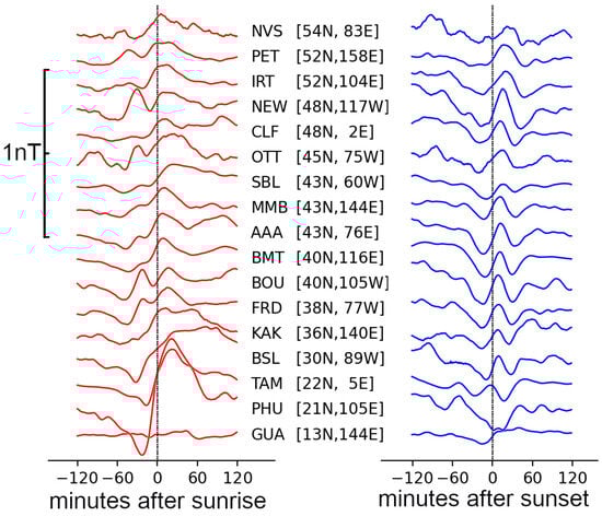
Figure 2.
Variations in the vertical Z component of the magnetic field with periods less than 1 h, averaged over 2000–2024 during sunrise and sunset for 17 observatories in Northern hemisphere. Sunrise and sunset moments are calculated for sea level altitude.
The hypothetical mechanism responsible for the creation of these St variations is the currents flowing along the terminator lines, separate from the Sq current system, and differing from it in a rather small width (Figure 3). Let us attempt to estimate the magnitude of the ionospheric current responsible for the creation of St variations. As already mentioned, the magnetic field St variations are extended along the terminator line, which means that causing them currents also moves along the terminator at its speed. When a meridional horizontal current flows through a thin conductor, the magnetic field will be created around it, the induction lines of which lie in a plane located vertically along the parallels [16]. Therefore, such a current will create disturbances only in the vertical Z and in the eastern Y component of the magnetic field [17]. In Figure 3, the direction of the current to poles is shown conditionally; the polarity of the additional variations in the magnetic field recorded on the earth’s surface depends on this direction.
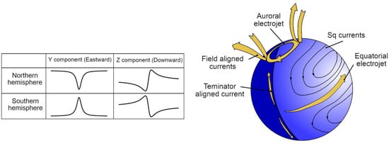
Figure 3.
Schematic representation of the main regular ionospheric current structures and terminator-aligned currents.
Figure 4 shows the calculations of the vertical Bz (positive direction–downward, like the Z component of the magnetic field) and the eastward By component of the magnetic field created by this current, in the time domain relative to the passage of this current moving at a speed of 1280 km/h (the speed of the terminator moving in a westward direction at a latitude of 40 degrees, the latitude of the Boulder Observatory).
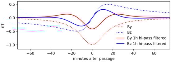
Figure 4.
Calculations of Y and Z magnetic field components for a horizontal meridional current of 1500 amperes flowing at an altitude of 300 km in the direction from the equator to the north.
These plots are constructed for a horizontal meridional current of 1500 Amperes at an altitude of 300 km from the equator to the north. The altitude and current strength were selected to correspond to a characteristic period of 20–40 min and a characteristic amplitude of 0.5 nT for St variations [1]. After applying a 1 h high-pass filter (as applied to the magnetic observatory measurement data), the magnetic field variations will appear as periodic oscillations. The dependence of the oscillation period on the current altitude allows for a rough estimate of the altitude of the electric current which create actual St variations. Thus, at an altitude of 300 km (the approximate height of the ionospheric F layer), the interval from the minimum to maximum phase will be approximately 20 min (Figure 5), which coincides with the similar interval for St variations (Figure 1). From this, we can conclude that the meridional current responsible for St variations in the magnetic field in mid-latitudes flows at the height of the ionospheric F layer, and its typical strength is approximately 1–2 thousand Amperes.
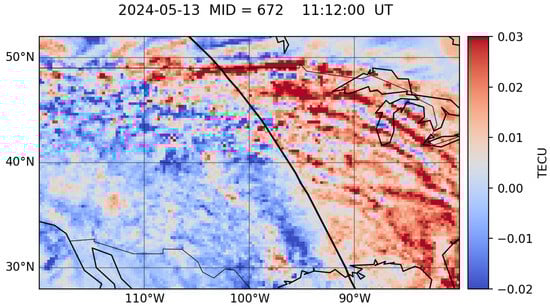
Figure 5.
TEC variations map on 13 May 2024. Black line shows morning terminator locations calculated for sea level altitude.
Next, we will try to detect any irregularity in the ionosphere corresponding to this current. To do this, we examined total electron content variations measured by ground-based GNSS receivers.
4. Results
For more than three hundred days in 2023 and 2024, TEC variation maps with a time resolution of 1 min were constructed for the region [30–50° N; 80–120° W]. Figure 5 shows an example of such a TEC variation map for 13 May 2024, at 11:12 UT. The morning terminator, calculated for sea level altitude, is marked with a line in the figure. MID means Minute in Day in UT time.
Examining dynamic maps of TEC variations for some days, it could be seen that before the line of the morning terminator, there is an elongated strip of increased electron concentration of a very small magnitude, a few hundredths of a TECU, located 20–30 min before the moment of passage of the terminator at sea level (5–7 degrees westward).
As can be seen from the figure, after the passage of the terminator (to the east of the terminator line), with the onset of day, numerous medium-scale traveling ionospheric disturbances (TIDs) are observed. Similar TIDs have been considered in several papers [8,18,19]. These waves are often called terminator waves [20,21,22], but they are not coherent (their phase pattern relative to the terminator line varies greatly depending on the local solar time and from day to day). Most likely, these waves, which are medium-scale TIDs, are created not by the motion of the terminator as a supersonic source of disturbances, but as a result of thermal tides in the atmosphere [10]. At the same time, in front of (to the west) the terminator line, a strip of increased electron concentration is observed that is stable relative to solar time and the terminator line. In a static image, the stability of this line relative to the terminator line is not obvious; for a better visual representation, we suggest viewing the animation of this map for this and other days [Figure S1]. The stability of this terminator-aligned TEC structure allows us to apply the method of superposing epochs relative to the terminator moment [23] to refine it, and by averaging the values for the entire period of the terminator’s passage through the region of 80–120° W, to obtain TEC variations that are coherent relative to the terminator moment. Figure 6 shows examples of TEC variations averaged relative to the morning terminator moment for several days.
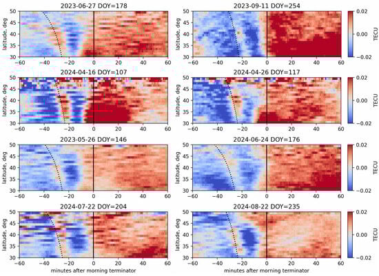
Figure 6.
Examples of clear pattern of morning pre-terminator irregularities in TEC. Dotted lines indicate morning terminator moments calculated for an altitude of 20 km. DOY means Day Of Year.
As can be seen from Figure 6, TEC variations contain a disturbance clearly associated with the morning terminator, but preceding it by 20–40 min, depending on latitude. Moreover, the peaks of this disturbance are in good agreement with the passage of the terminator at an altitude of 20 km (shown by dotted lines in the figure). The passage times and durations of these disturbances are in good agreement with the St variations in the Boulder BOU magnetic observatory (Figure 1). This allows us to assume that an electric current, which is responsible for the presence of St variations in the magnetic observatory data, passes through the ionospheric layer containing the TEC disturbances shown in Figure 5 and Figure 6.
5. Discussion and Conclusions
The paper shows that a longitudinal structure of increased electron density elongated along the morning solar terminator line has been detected in the ionospheric total electron content data calculated from dual-frequency GNSS receivers located across the continental United States (at latitudes ranging from 30 to 50 degrees north). Although the amplitude of this structure is extremely small, amounting to only a few hundredths of a TECU, it can be consistently observed with a sufficiently dense array of receivers and a fairly simple data processing method based on the coherent accumulation of disturbances fixed in time as they pass through the terminator. With appropriate processing, this structure can certainly be detected using the system [24]. This structure is not observed every day; in the data of 340 days in 2023–2024, we were able to clearly identify it (meaning as clearly as it can be seen in Figure 6) on average on 20% of days, which is due to the fact that this structure is difficult to identify against the background of other ionospheric disturbances. We have processed data for 2023–2024, which included the maximum of the 25th cycle of solar activity, and we assume that a large number of magnetic storms, and therefore disturbed ionosphere, are the reason for such a percentage of clearly visible disturbances from the terminator. But another possibility is that this effect is not regular. There are many magnetically quiet days when no clear pattern of TEC disturbances along the terminator is visible. However, the small number of processed days does not yet allow us to draw a conclusion about the seasonal dependence of the probability and amplitude of this structure, as well as its dependence on space weather factors.
For the evening terminator, a similar structure was not detected in the TEC data. We assume that the reason for this is that during the passage of the evening terminator in the ionosphere, there is a large number of background moving ionospheric disturbances of the AGW type [8], against the background of which the weak structure from the solar terminator is lost.
The transit time (20–30 min before the solar terminator), orientation (along the terminator line), and corresponding direction and velocity indicate that this ionospheric structure likely contains a longitudinal current responsible for the occurrence of St variations in the magnetic field. Of course, the question of the connection between this structure of increased electron concentration in the ionosphere and the previously detected magnetic field variations [1] associated with the passage of the solar terminator remains open. However, in our opinion, this is the first confirmed evidence of the presence of coherent irregularities in the ionosphere, moving together with the solar terminator.
Possible mechanisms for the formation of this structure, in our opinion, could be a shock wave generated by the terminator’s motion as a supersonic disturbance [9,12] and causing a redistribution of the electron density or additional ionization in the ionosphere. To clarify the mechanisms of formation of this structure and the ionospheric current responsible for the creation of St variations, additional experimental confirmations at different latitudes and with high sensitivity are needed. In the Southern Hemisphere, there are a relatively small number of magnetic observatories, and therefore, the symmetry of Sq variations in the Northern and Southern Hemispheres is difficult to establish. The same applies to the availability of GNSS receivers in the Southern Hemisphere and the possibility of studying ionospheric TEC. Satellite magnetic field measurement data obtained on SWARM satellites is difficult to apply to the study of the terminator due to the peculiarity of the satellites’ orbits—most of the time they fly along the terminator line, rather than intersecting it, which makes the search for this effect a major challenge.
The least understood time interval is the detected time interval between the moment of terminator passage at ground level and the moment of passage of the St variations in the magnetic field (this moment for the Z field component corresponds to a reversal of the magnetic disturbance’s polarity), as well as the moment of passage of the structure of increased electron density in the GNSS TEC data. The coincidence of this structure in the ionosphere with the moment of terminator passage at an altitude of 20 km, indicated in Figure 4, does not necessarily indicate that the change in electron density occurs at this altitude with the first rays of the sun. However, it does indicate that the latitudinal dependence of the moment of passage of this structure follows the latitudinal dependence of the change in illumination during terminator passage.
It should also be noted that all the variations considered, both the magnetic field St variations and the electron density variations, have very small amplitudes and are not distinguishable by eye when visually comparing magnetic and TEC time series for any given period. Their detection requires methods to enhance the signal-to-noise ratio, such as the epoch superposition method used in this study.
Supplementary Materials
The following supporting information can be downloaded at: https://www.mdpi.com/article/10.3390/atmos16101217/s1, Figure S1: TEC variations map during the passage of the morning solar terminator on 13 May 2024. Black line shows morning terminator locations calculated for sea level altitude.
Author Contributions
Conceptualization, A.A. and V.S.; methodology, A.A. and V.S.; software, A.A., Y.C. and S.U.; validation, A.A. and V.K.; formal analysis, V.S.; investigation, A.A.; resources, V.K.; data curation, A.A., Y.C. and S.U.; writing—original draft preparation, A.A.; writing—review and editing, V.S.; visualization, Y.C.; supervision, V.S.; project administration, A.A. All authors have read and agreed to the published version of the manuscript.
Funding
This study was funded by the Science Committee of the Ministry of Science and Higher Education of the Republic of Kazakhstan, grant project AP19680174 “The study of the ionospheric disturbances dynamics using GNSS tomography methods”.
Institutional Review Board Statement
Not applicable.
Informed Consent Statement
Not applicable.
Data Availability Statement
The work is based on GNSS RINEX data provided by the NOAA Continuously Operating Reference Station (CORS) Network (NCN), managed by NOAA/National Geodetic Survey via https://geodesy.noaa.gov/CORS/ (accessed on 16 October 2025), and on data on Earth’s magnetic field measurements, carried out at geomagnetic observatories of the IAGA standard and provided by the INTERMAGNET network https://intermagnet.org/data_download.html (accessed on 16 October 2025).
Conflicts of Interest
The authors declare no conflicts of interest. The funders had no role in the design of the study; in the collection, analyses, or interpretation of data; in the writing of the manuscript; or in the decision to publish the results.
Abbreviations
The following abbreviations are used in this manuscript:
| CORS | Continuously Operating Reference Station |
| GNSS | Global Navigation Satellite System |
| IAGA | The International Association of Geomagnetism and Aeronomy |
| NOAA | National Oceanic and Atmospheric Administration |
| Sq | Solar quiet |
| TEC | Total Electron Content |
| TECU | Total Electron Content Unit |
References
- Andreyev, A.; Somsikov, V.; Kapytin, V.; Chsherbulova, Y. Solar terminator related variations in geomagnetic field. J. Atmos. Sol.-Terr. Phys. 2025, 271, 106517. [Google Scholar] [CrossRef]
- Yamazaki, Y.; Maute, A. Sq and EEJ—A review on the daily variation of the geomagnetic field caused by ionospheric dynamo currents. Space Sci. Rev. 2017, 206, 299–405. [Google Scholar] [CrossRef]
- Soares, G.; Yamazaki, Y.; Cnossen, I.; Matzka, J.; Pinheiro, K.J.; Morschhauser, A.; Alken, P.; Stolle, C. Evolution of the geomagnetic daily variation at Tatuoca, Brazil, from 1957 to 2019: A transition from Sq to EEJ. J. Geophys. Res. Space Phys. 2020, 125, e2020JA028109. [Google Scholar] [CrossRef]
- Mann, R.J.; Schlapp, D.M. The equatorial electrojet and the day-ato-day variability of Sq. J. Atmos. Terr. Phys. 1988, 50, 57–62. [Google Scholar] [CrossRef]
- Chulliat, A.; Matzka, J.; Masson, A.; Milan, S. Key ground-based and space-based assets to disentangle magnetic field sources in the Earth’s environment. Space Sci. Rev. 2017, 206, 29–60. [Google Scholar] [CrossRef]
- Afraimovich, E.; Astafyeva, E.; Demyanov, V.; Edemskiy, I.; Gavrilyuk, N.; Ishin, A.B.; Kosogorov, E.A.; Leonovich, L.A.; Lesyuta, O.S.; Palamartchouk, K.S.; et al. A review of GPS/GLONASS studies of the ionospheric response to natural and anthropogenic processes and phenomena. J. Space Weather Space Clim. 2013, 3, A27. [Google Scholar] [CrossRef]
- Komjathy, A.; Yang, Y.; Meng, X.; Verkhoglyadova, O.; Mannucci, A.J.; Langley, R.B. Review and perspectives: Understanding natural-hazards-generated ionospheric perturbations using GPS measurements and coupled modeling. Radio Sci. 2016, 51, 951–961. [Google Scholar] [CrossRef]
- Andreyev, A.; Kapytin, V.; Yakovets, A.; Chsherbulova, Y. A Method for Determining Parameters of Mid-Scale Traveling Ionospheric Disturbances. Sensors 2025, 25, 5377. [Google Scholar] [CrossRef]
- Beer, T. Supersonic generation of atmospheric waves. Nature 1973, 242, 34–35. [Google Scholar] [CrossRef]
- Miyoshi, Y.; Fujiwara, H.; Forbes, J.M.; Bruinsma, S.L. Solar terminator wave and its relation to the atmospheric tide. J. Geophys. Res. 2009, 114, A07303. [Google Scholar] [CrossRef]
- Zhu, L.; Schunk, R.W.; Eccles, V.; Scherliess, L.; Sojka, J.J.; Gardner, L. Terminator field-aligned current system: Its dependencies on solar, seasonal, and geomagnetic conditions. J. Atmos. Sol. Terr. Phys. 2017, 164, 10–17. [Google Scholar] [CrossRef]
- Somsikov, V.M. Solar terminator and dynamic phenomena in the atmosphere: A review. Geomagn. Aeron. 2011, 51, 723–735. [Google Scholar] [CrossRef]
- Lizunov, G.; Fedorenko, A.; Bankov, L.; Vassileva, A.K. Atmospheric gravity waves associated with moving solar terminator through Earth’s upper atmosphere. Aero. Res. Bulgaria 2009, 23, 36–49. [Google Scholar]
- Karpov, I.V.; Bessarab, F.S. Model studying the effect of the solar terminator on the thermospheric parameters. Geomagn. Aeron. 2008, 48, 209–219. [Google Scholar] [CrossRef]
- Forbes, J.M.; Bruinsma, S.L.; Miyoshi, Y.; Fujiwara, H. A solar terminator wave in thermosphere neutral densities measured by the CHAMP satellite. Geophys. Res. Lett. 2008, 35, L14802. [Google Scholar] [CrossRef]
- Kikuchi, T.; Hashimoto, K.K. Transmission of the electric fields to the low latitude ionosphere in the magnetosphere-ionosphere current circuit. Geosci. Lett. 2016, 3, 4. [Google Scholar] [CrossRef]
- Tsunomura, S. Numerical analysis of global ionospheric current system including the effect of equatorial enhancement. Ann. Geophys. 1999, 17, 692–706. [Google Scholar] [CrossRef]
- Moges, S.T.; Sherstyukov, R.O.; Kozlovsky, A.; Ulich, T.; Lester, M. Statistics of traveling ionospheric disturbances at high latitudes using a rapid-run ionosonde. J. Geophys. Res. Space Phys. 2024, 129, e2023JA031694. [Google Scholar] [CrossRef]
- Kotake, N.; Otsuka, Y.; Ogawa, T.; Tsugawa, T.; Saito, A. Statistical study of medium-scale traveling ionospheric disturbances observed with the GPS networks in Southern California. Earth Planets Space 2007, 59, 95–102. [Google Scholar] [CrossRef]
- Cheremnykh, O.; Fedorenko, A.; Voitsekhovska, A.; Selivanov, Y.; Ballai, I.; Verth, G.; Fedun, V. Atmospheric waves disturbances from the solar terminator according to the VLF radio stations data. Adv. Space Res. 2023, 72, 4825–4835. [Google Scholar] [CrossRef]
- Afraimovich, E.L.; Edemsky, I.K.; Voeykov, S.V.; Yasukevich, Y.V.; Zhivetiev, I.V. MHD nature of ionospheric wave packets generated by the solar terminator. Geomagn. Aeron. 2010, 50, 79–95. [Google Scholar] [CrossRef]
- Reinisch, B.; Galkin, I.; Belehaki, A.; Paznukhov, V.; Huang, X.; Altadill, D.; Buresova, D.; Mielich, J.; Verhulst, T.; Stankov, S.; et al. Pilot Ionosonde Network for Identification of Traveling Ionospheric Disturbances. Radio Sci. 2018, 53, 365–378. [Google Scholar] [CrossRef]
- Fedorenko, A.K.; Kryuchkov, E.I.; Voitsekhovska, A.D.; Cheremnykh, O.K.; Zhuk, I.T. Wave atmospheric disturbances from the solar terminator in the morning and evening hours based on measurements of amplitudes of VLF radio signals. Kinemat. Phys. Celest. Bodies 2024, 40, 295–305. [Google Scholar] [CrossRef]
- Inchin, P.; Snively, J.; Zettergren, M. System for Rapid Analysis of Ionospheric Dynamics Based on GNSS TEC Signals, Version 1; Embry-Riddle Aeronautical University: Daytona Beach, FL, USA, 2024. [Google Scholar] [CrossRef]
Disclaimer/Publisher’s Note: The statements, opinions and data contained in all publications are solely those of the individual author(s) and contributor(s) and not of MDPI and/or the editor(s). MDPI and/or the editor(s) disclaim responsibility for any injury to people or property resulting from any ideas, methods, instructions or products referred to in the content. |
© 2025 by the authors. Licensee MDPI, Basel, Switzerland. This article is an open access article distributed under the terms and conditions of the Creative Commons Attribution (CC BY) license (https://creativecommons.org/licenses/by/4.0/).