Article

Causes of Summer Ozone Pollution Events in Jinan, East China: Local Photochemical Formation or Regional Transport?

1
School of Environmental Science and Engineering, Qilu University of Technology (Shandong Academy of Sciences), Jinan 250353, China
2
Jinan Eco-Environmental Monitoring Center of Shandong Province, Jinan 250101, China
3
Ecology Institute of Shandong Academy of Sciences, Qilu University of Technology (Shandong Academy of Sciences), Jinan 250103, China
*
Author to whom correspondence should be addressed.
Atmosphere 2024, 15(2), 232; https://doi.org/10.3390/atmos15020232
Submission received: 17 January 2024 / Revised: 4 February 2024 / Accepted: 13 February 2024 / Published: 15 February 2024
(This article belongs to the Special Issue Ozone Pollution and Effects in China)

Abstract

:
Simultaneous measurements of atmospheric volatile organic compounds (VOCs), conventional gases and meteorological parameters were performed at an urban site in Jinan, East China, in June 2021 to explore the formation and evolution mechanisms of summertime ozone (O3) pollution events. O3 Episode Ⅰ, O3 Episode II, and non-O3 episodes were identified based on the China Ambient Air Quality Standards and the differences in precursor concentrations. The O3 concentrations in Episode I and Episode II were 145.4 μg/m3 and 166.4 μg/m3, respectively, which were significantly higher than that in non-O3 episode (90 μg/m3). For O3 precursors, VOCs and NOx concentrations increased by 48% and 34% in Episode I, and decreased by 21% and 27% in Episode II compared to non-O3 episode days. The analysis of the m,p-xylene to ethylbenzene ratio (X/E) and OH exposure demonstrated that the aging of the air masses in Episode II was significantly higher than the other two episodes, and the differences could not be explained by localized photochemical consumption. Therefore, we speculate that the high O3 concentrations in Episode II were driven by the regional transport of O3 and its precursors. Backward trajectory simulations indicated that the air masses during Episode II were concentrated from the south. In contrast, the combination of high precursor concentrations and favorable meteorological conditions (high temperatures and low humidity) led to an excess of O3 in Episode I. Positive matrix factorization (PMF) model results indicated that increased emissions from combustion and gasoline vehicle exhausts contributed to the elevated concentrations of VOCs in Episode I, and solvent usage may be an important contributor to O3 formation. The results of this study emphasize the importance of strengthening regional joint control of O3 and its precursors with neighboring cities, especially in the south, which is crucial for Jinan to mitigate O3 pollution.

1. Introduction

In recent years, the air pollution problem has been increasingly exposed due to the accelerated urbanization in China. To achieve better air quality, the Chinese government has implemented a series of actions to control air pollution since 2013 [1,2]. PM2.5 pollution has been significantly reduced throughout China; however, ozone (O3) concentrations have continued to increase in urban areas due to the combination of increased emissions of volatile organic compounds (VOCs), decreased emissions of nitrogen oxides (NOX) and reduced aerosol effects [3,4,5]. The pollution of O3 is already an important constraint to the continuous improvement of China’s air quality.
Tropospheric O3 formation is mainly dominated by photochemical reactions of VOCs and NOX [6]. In addition to precursors, O3 pollution is also associated with meteorological conditions such as relative humidity, sunlight, temperature and atmospheric pressure [7,8], and is also affected by transmission in the vertical direction or from neighboring cities [9,10]. These factors make O3 pollution control complex.
Unlike “hot spots” such as Beijing-Tianjin-Hebei [11,12,13], Yangtze River Delta [14,15] and Pearl River Delta [16,17], studies on O3 pollution in Shandong Province are relatively limited. As one of the “2+26” cities in Beijing-Tianjin-Hebei and neighboring areas, Jinan, the capital city of Shandong Province, is facing serious air pollution problems, and was ranked 154th among 168 key cities in the country’s air quality ranking in June 2021 (https://www.mee.gov.cn/ywdt/xwfb/202107/t20210719_848943.shtml, accessed 9 August 2023). A comprehensive analysis of ozone pollution in Jinan is urgently needed in order to mitigate adverse effects on ambient air quality in the Beijing-Tianjin-Hebei region.
In this study, O3 and its precursors were continuously monitored at an urban site in Jinan. The pollution characteristics of O3, VOCs, NOX as well as the differences in meteorological conditions in different O3 pollution episodes were analyzed; the aging degree of air masses was identified based on specific VOC ratios; the influence of regional transport on ozone pollution was explored by backward trajectory, and source apportionment of VOCs using the PMF model was performed. This study reveals the characteristics of different types of O3 pollution and their formation mechanisms, which can provide scientific support for O3 pollution control in Jinan.

2. Materials and Methods

2.1. Measurements

The field measurements were performed from 1 June to 30 June 2021, on the roof of the Jinan monitoring station (36.67° N, 117.06° E) at a height of about 20 m (Figure S1). The location of the sampling site is on the west side of the Shanda Road and is surrounded by buildings without any obvious obstructions. The site is mainly affected by traffic and residential sources and is a typical urban site that can represent the air pollution situation of Jinan City.
VOCs were monitored with an on-line gas chromatograph mass spectrometer/flame ionization detection system (GC-MS/FID), with a time resolution of 1 h. Detailed descriptions of this instrument can be obtained from another reference [18]. Briefly, the ambient air samplings were collected at ultra-low temperatures (−150 °C) through two parallel sampling channels, followed by thermal desorption. Low-carbon hydrocarbons (C2–C5) were separated with a Al2O3/KCl PLOT column and analyzed using FID, while high-carbon hydrocarbons (C5–C12), halogenated hydrocarbons and OVOCs were determined via MS after separation on a DB-624 column. The detection limits were in the range of 0.01–0.10 ppb for all measured species.
Ambient nitric oxide (NO) and nitrogen dioxide (NO2) concentrations were measured using a commercial NO-NO2-NOX analyzer (Teledyne API, USA, Model 200E). O3 concentrations were determined with a commercial instrument using UV absorption (Teledyne API, USA, Model 400E). Additionally, meteorological parameters were obtained from the Jinan Meteorological Bureau.

2.2. Ozone Formation Potential (OFP)

The maximum incremental reactivity (MIR) method is widely applied to evaluate the contribution of individual VOCs to the ozone formation potential (OFP). The formula for calculating the OFP for each VOC is as follows:
O F P i = C o n c i × M I R i
where Conc (i) is the concentration of the ith VOC, and MIR (i) is the maximum incremental reactivity coefficient of the ith VOC, which can be obtained from [19]. The OFP calculated with this method only reflects the maximum contribution of a specific VOC species to O3 concentration under optimum laboratory conditions [20], and the OFP does not represent the absolute amount of O3 contributed by the species in the actual environment [21]. The most important implication of this method is to identify the key VOC species for O3 production rather than the amount of O3 specifically produced.

2.3. OH Exposure

Specific ratios of VOCs are commonly adopted to evaluate the photochemical age or OH exposure of air masses [22,23,24]. This study calculated OH exposure according to the ratio of m,p-xylene to ethylbenzene (X/E), and the equation used is shown as follows:
O H Δ t = 1 k X k E × l n X E t = t 0 l n X E t = t ,
where   O H Δ t represents the OH exposure, i.e., the multiplication of the OH radical concentration and the reaction time. k X and k E denote the OH reaction rate constants for m,p-xylenes (X) and ethylbenzene (E), respectively. X E t = t 0 a n d   X E t = t are the initial emission ratio and the observed ratio of X/E, respectively.

2.4. Positive Matrix Factorization (PMF) Model

PMF is commonly applied to evaluate the main sources of VOCs based on an analysis of the measured data at receptors sites and without direct measurements of source profiles [25,26,27]. The EPA’s PMF 5.0 model was adopted in this study to analyze each source’s contribution to VOCs. The detailed description of this model can be found in the User Guide (U.S. Environmental Protection Agency, Washington, 2014) and our previous study [28]. In this work, 24 species were entered into the model, and data completeness was greater than 75% for each species, with valid data more than 65% (Conc. ≥ MDL) and signal-to-noise ratio (S/N) larger than 1.5. The factors were tested from 4 to 7. The Q/Qexp values and the Fpeak values from −1.0 to 1.0 (step of 0.1) were used to obtain the best solution. Finally, 6 factors were selected.

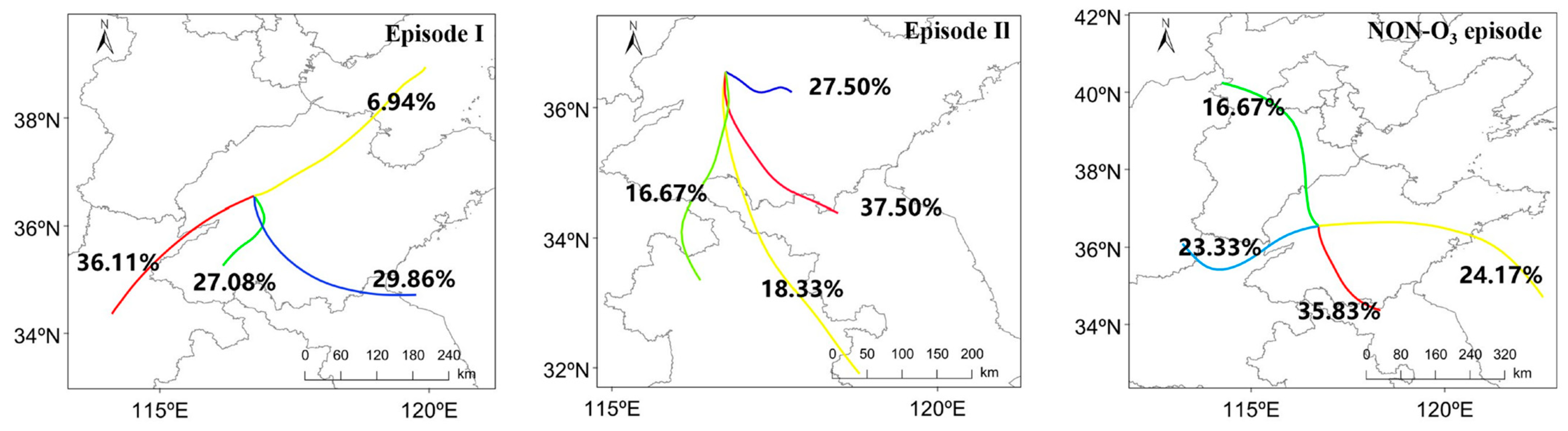
2.5. Backward Trajectory Simulation

The HYSPLIT backward trajectory model (https://www.ready.noaa.gov/HYSPLIT_traj.php, accessed 7 March 2023) developed by the National Oceanic and Atmospheric Administration (NOAA) was used in this study to assess the impact of air mass transport on summer O3 pollution in Jinan. Weather data were obtained from the NOAA Air Resources Laboratory Global Data Assimilation System (GDAS) archives. The backward trajectory of air masses 500 m above the ground was simulated for 24 h with a time resolution of 1 h. Cluster analysis was then performed using the Trajstat module in MeteoInfo 3.3.0 software to derive the results of the air mass trajectory analysis.

3. Results and Discussion

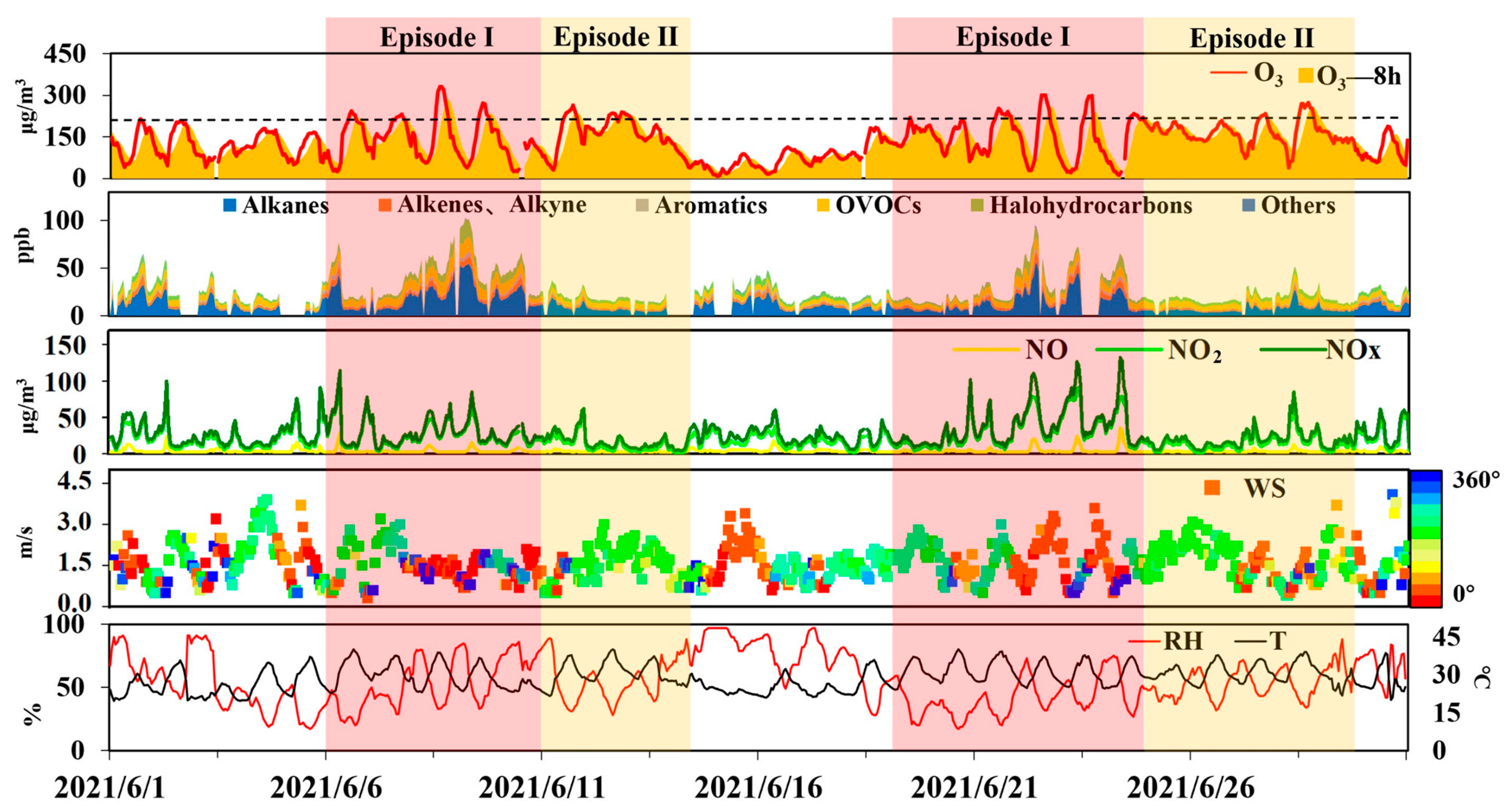
3.1. Characteristics of Meteorological Parameters and O3 Precursors during Different O3 Episodes

3.1.1. General Description

The time series of trace gases, meteorological parameters and VOCs observed in Jinan from 1 June to 30 June 2021 are shown in Figure 1. The black line in O3 time series represents the threshold of the 1 h average O3 concentration according to the Chinese National Air Quality Standard Grade II (200 μg/m3). As presented in Figure 1, the urban area of Jinan suffered from severe O3 pollution in June. Episodes with the 1 h average O3 concentration exceeding the standard limit for more than two continuous days were identified as O3 Episode I: 6–10 June and 19–24 June. Notably, 1 h average O3 concentrations on 11–13 June and 25–29 June were also significantly above the ambient air quality standard but were separately defined as O3 Episode II due to the lower precursor concentrations (VOCs and NOX) and higher O3 concentrations during nights. In addition, other days were classified as non-O3 episodes. The maximum concentrations of 1 h average O3 reached 330.1 μg/m3 and 273.2 μg/m3 in Episode I and Episode II, respectively.
The average values of VOCs, conventional gases and meteorological parameters for different ozone pollution episodes in June 2021 are shown in Table 1. The average O3 concentrations in Episode I and Episode II were 145.4 μg/m3 and 166.4 μg/m3, respectively, which is about 1.6 and 1.8 times higher than those in the non-O3 episode (90 μg/m3). VOCs and NOX concentrations increased by 48% and 34% in Episode I compared to the non-O3 episode. A previous study showed that O3 generation in the urban area of Jinan was VOC-limited in the morning and shifted to a VOCs-NOX transition regime in the afternoon [29]. The relatively higher VOCs and NOX concentrations suggested that the local photochemical reaction formations may significantly contribute to the elevated O3 concentrations in Episode I. It should be noted that the concentrations of VOCs and NOX in Episode II exhibited opposite variation characteristics with Episode I. The VOCs and NOX decreased by 21% and 27% in Episode II compared to the non-O3 episode.
The average temperatures of O3 Episode I and Episode II were 4.5 °C and 4.9 °C higher than the non-O3 episode. The higher temperatures typically accelerate the photochemical generation of O3. The relative humidity (RH) was lower for ozone episodes than that of the non-O3 episode, and the low RH favored O3 production. However, it should be mentioned that the differences in RH between O3 episodes could not fully interpret the differences in O3 concentrations. For example, 8–10 June was characterized by high RH (the maximum RH exceeded 80% for three consecutive days) but shows relatively high O3 concentrations. The wind speeds were comparable in both O3 and non-O3 episodes. The wind direction varied significantly among different types of O3 episodes, in which the southwestern winds were particularly concentrated during Episode II. Combined with the characteristics of O3 precursor concentrations, it was preliminary speculated that the high O3 concentrations in Episode II might be related to the regional transport from the southwestern direction.

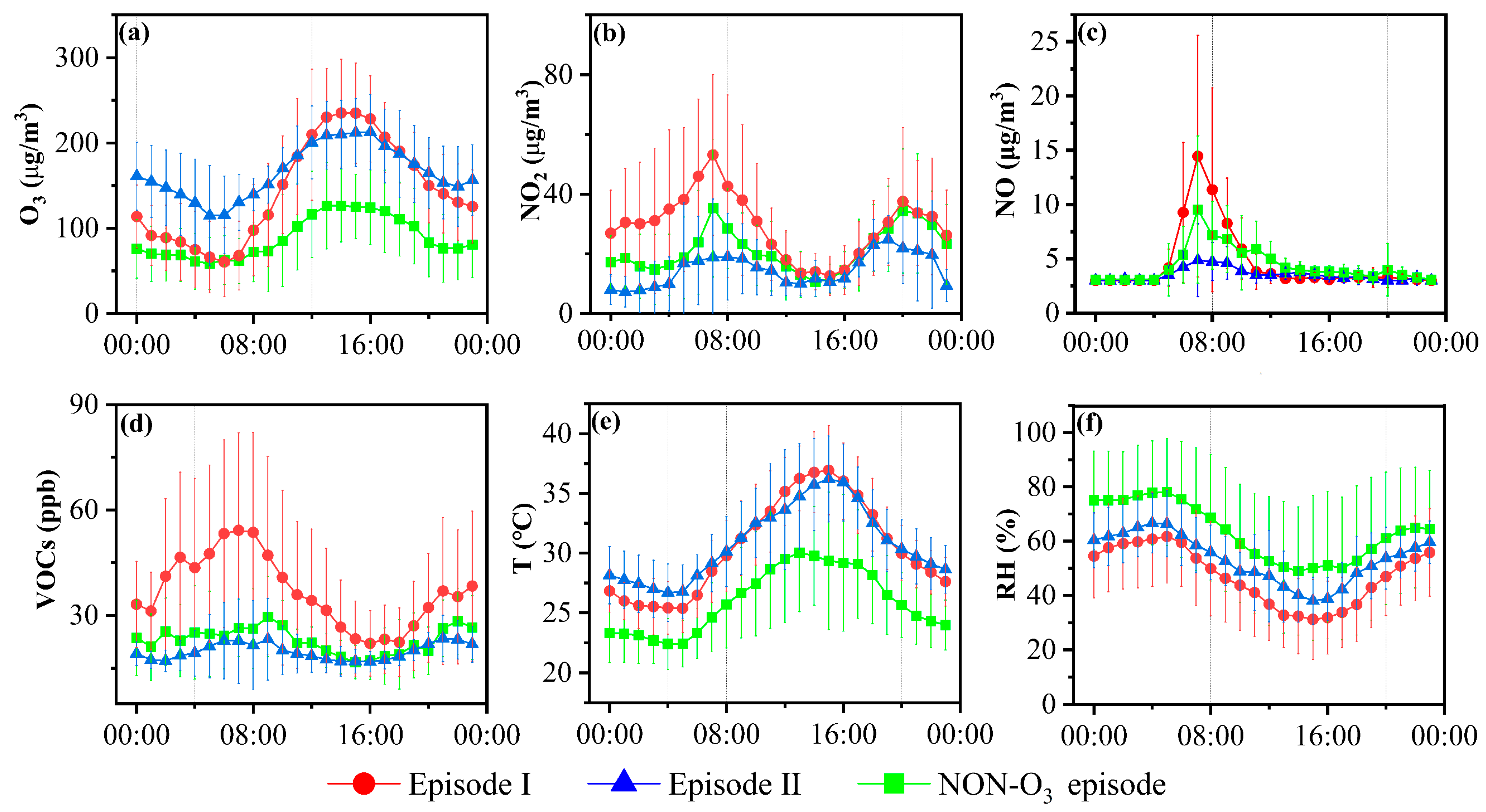
3.1.2. Diurnal Variations

Diurnal variations of O3, NO2, NO, VOCs, RH and temperature during different O3 episodes are shown in Figure 2. As can be seen, the daily variations of O3 showed a single-peaked distribution for both O3 and non-O3 episodes. The O3 concentrations reached their lowest values at 06:00, with 58.8 μg/m3, 114.8 μg/m3 and 66.1 μg/m3 in Episode I, Episode Ⅱ and non-O3 episode, respectively. With the enhancement of solar radiation, the O3 concentrations started to increase rapidly, peaking at around 15:00, and then decreased, with relatively lower concentrations at night. Compared with Episode Ⅰ and non-O3 episode, the nighttime (00:00–06:00) O3 concentrations increased by 66% and 107% in Episode Ⅱ. Lower NO concentrations may have contributed to the high nighttime O3 levels in Episode II, since they can mitigate the titration effects of O3.
The diurnal variations of VOCs and NO2 showed different patterns with O3. Relatively high concentrations of VOCs and NO2 were identified in the morning (07:00) and evening (20:00) rush hours, which implied the influence of vehicle emission sources. The photochemical consumption of VOCs and NO2 increased with the solar radiation enhancement, and the minimum values occurred around 15:00. The overall VOCs and NO2 concentrations were lower in Episode Ⅱ, and the variations were more moderate in the morning and evening rush hours. This may be due to the fact that Episode Ⅱ was mainly concentrated during weekends, with significantly less traffic during rush hours. The temperature was noticeably lower, and the RH was higher during non-O3 episodes compared to ozone episodes. In addition, Episode Ⅱ was influenced by several rainfall events. Overall, meteorological factors were unfavorable for ozone production in non-O3 episodes.

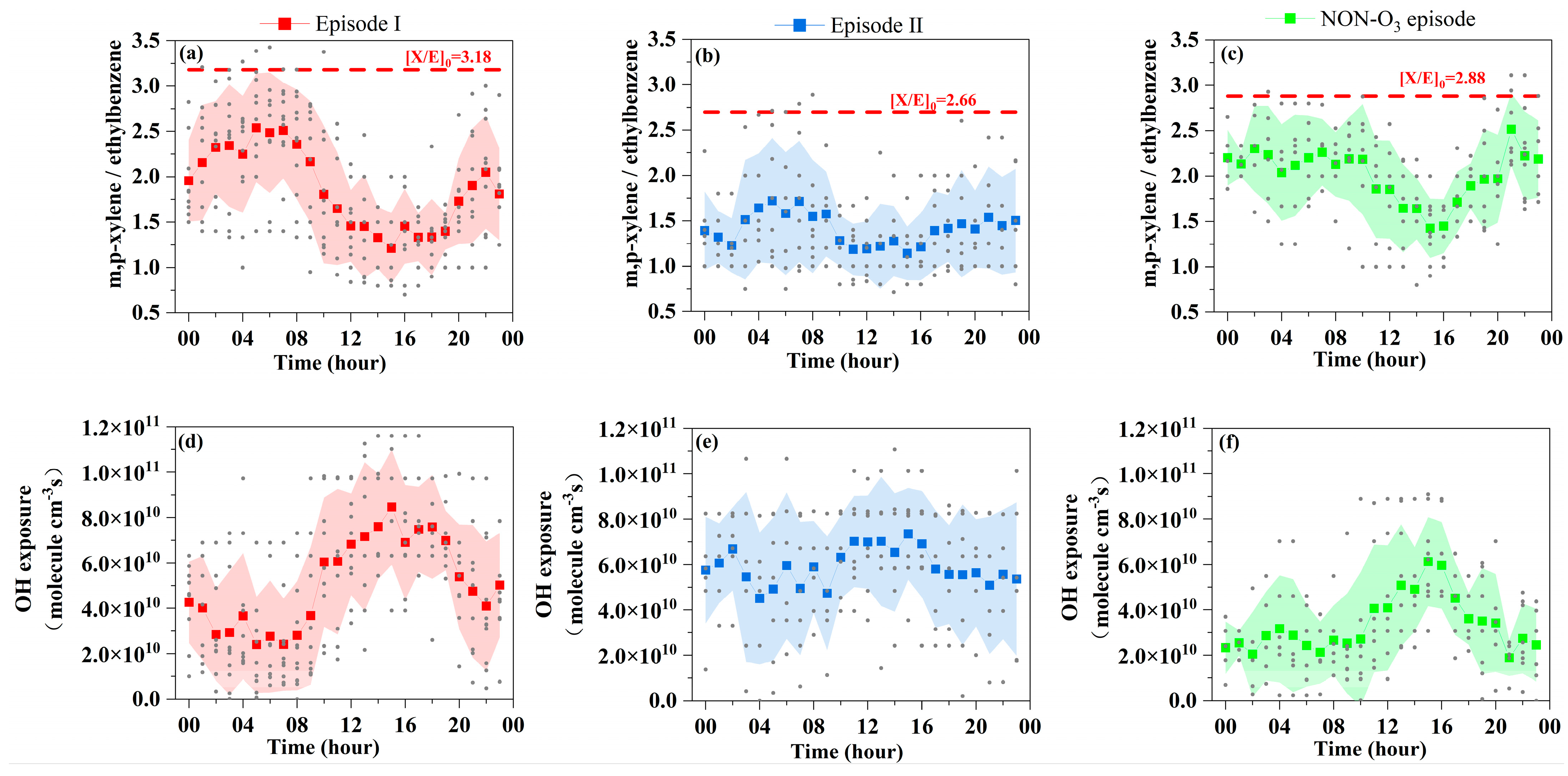
3.2. Aging of Air Masses in Different O3 Pollution Episodes

The m,p-xylene to ethylbenzene ratio (X/E) was widely applied to evaluate the photo-chemical aging of air masses [23,24]. The emission sources of m,p-xylene and ethylbenzene are similar [30], but the reactivity of m,p-xylene with OH radicals (kOH = 18.9 × 10⁻¹² cm3 molecule−1 s−1) is much faster than that of ethylbenzene (kOH = 7 × 10⁻¹² cm3 molecule−1 s−1) [31]. Therefore, the lower X/E ratio indicates the higher level of air mass aging. As shown in Figure 3a–c, the initial emission ratios of X/E in Episode Ⅰ, Episode Ⅱ and non-O3 episode were 3.18, 2.66 and 2.88, respectively, and the mean values of X/E were 1.88, 1.41 and 2.01, respectively. The lowest X/E value for Episode Ⅱ demonstrated the highest aging of the air masses compared to other periods. From the daily variations, the X/E decreased significantly from 9:00 to 15:00 during Episode Ⅰ and the non-O3 episode, which suggested a substantial photochemical consumption of VOCs during these periods. In contrast, the variations of X/E for Episode Ⅱ was not clear, meaning a weaker local photochemical consumption of VOCs. The daily variations of OH exposure was negatively correlated with X/E ratios (Figure 3d–f). Episode Ⅱ had the maximum average OH exposure, but the daily variation was not remarkable compared to other episodes. Overall, the highest aging of the air masses in Episode Ⅱ could not be explained by local photochemical depletion, and we speculate that this may be driven by the long-distance transport of the air masses.

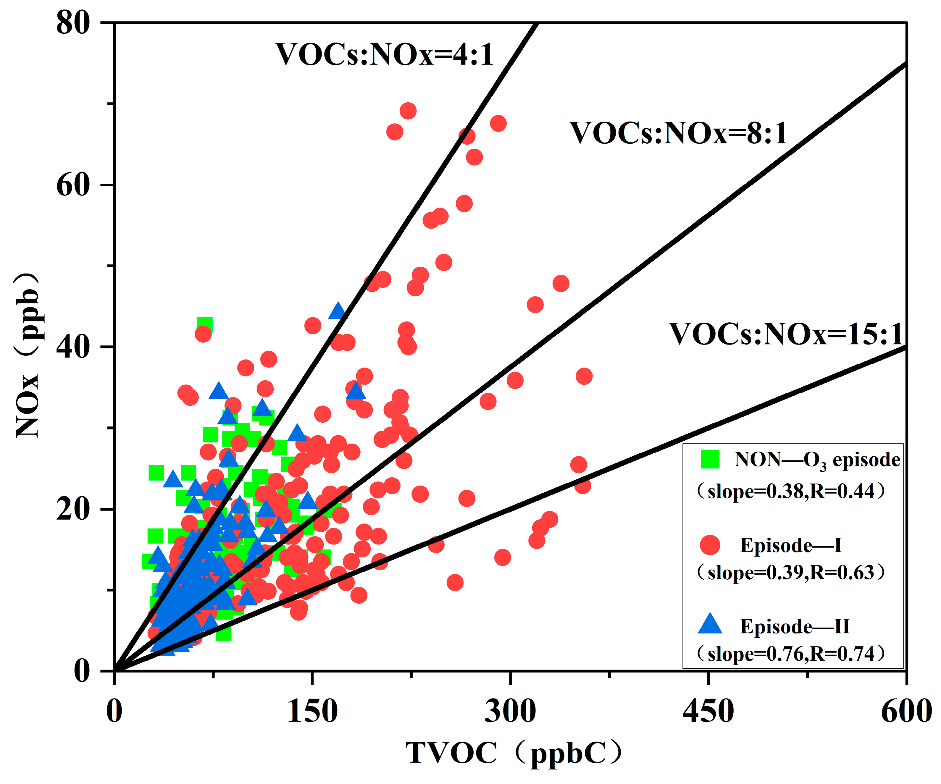
3.3. Relationship of VOC/NOX Ratios to O3 Generation Regime

Previous studies have shown that ozone formation is highly non-linear with its precursors [32,33]. Assessing whether O3 is limited by VOCs or NOX concentrations is especially important for the determination of regional air pollution control strategies. The VOCs/NOX ratios have been frequently applied to identify O3 formation regimes [34,35]. For instance, the ozone pollution numerical simulations in Los Angeles during the 1980s revealed that ozone formation transitioned from VOC-limited to NOX-limited when the ratio of VOCs to NOX was 8:1 [36]. In China, if the ratio of VOCs/NOX is below 4:1, O3 generation is mainly regulated by VOCs, and it is mainly limited by NOX when the ratio of VOCs to NOX is above 15:1. The production of O3 is controlled by both VOCs and NOX when the ratio of VOCs/NOX is between 4:1 and 15:1 [37]. As shown in Figure 4, the majority of the VOCs/NOX ratios for different O3 episodes were between 4:1 and 15:1 (averaging 7.5:1, 7.1:1 and 6.3 for Episode Ⅰ, Episode Ⅱ and non-O3 Episode, respectively), indicating that the generation of O3 in urban Jinan in summer was co-limited by VOCs and NOX. This was consistent with the results of O3-VOCs-NOX sensitivity studies during O3 pollution days in urban areas in Zhengzhou [38], Nanjing [39] and Guangzhou [40]. It should be noted that this study determined the ozone generation regime in the urban area of Jinan using the VOCs/NOX ratio method based on only one month of observational data. In the future, photochemical models should be employed to analyze the effects of VOCs and NOX in relation to O3 formation to obtain more reliable results.

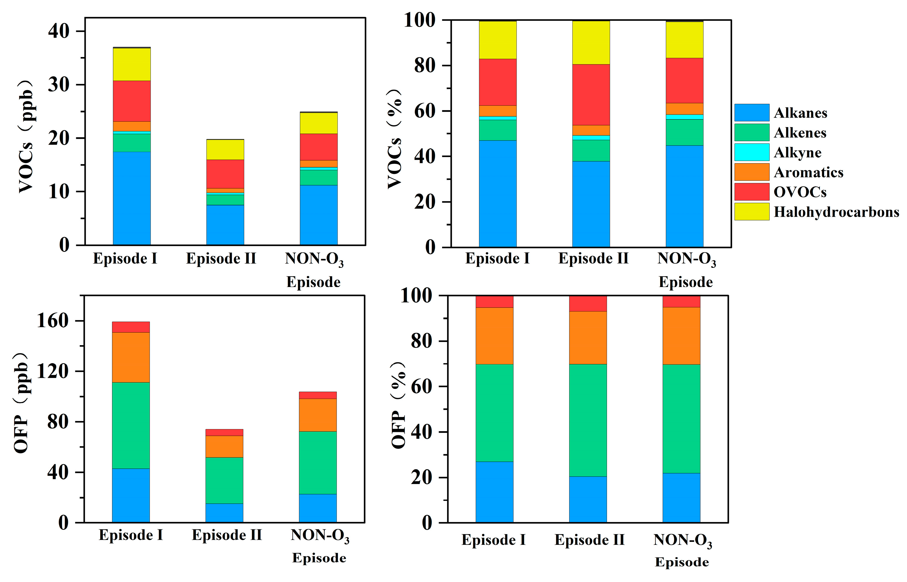
3.4. Reactivity and Source Apportionment of VOCs

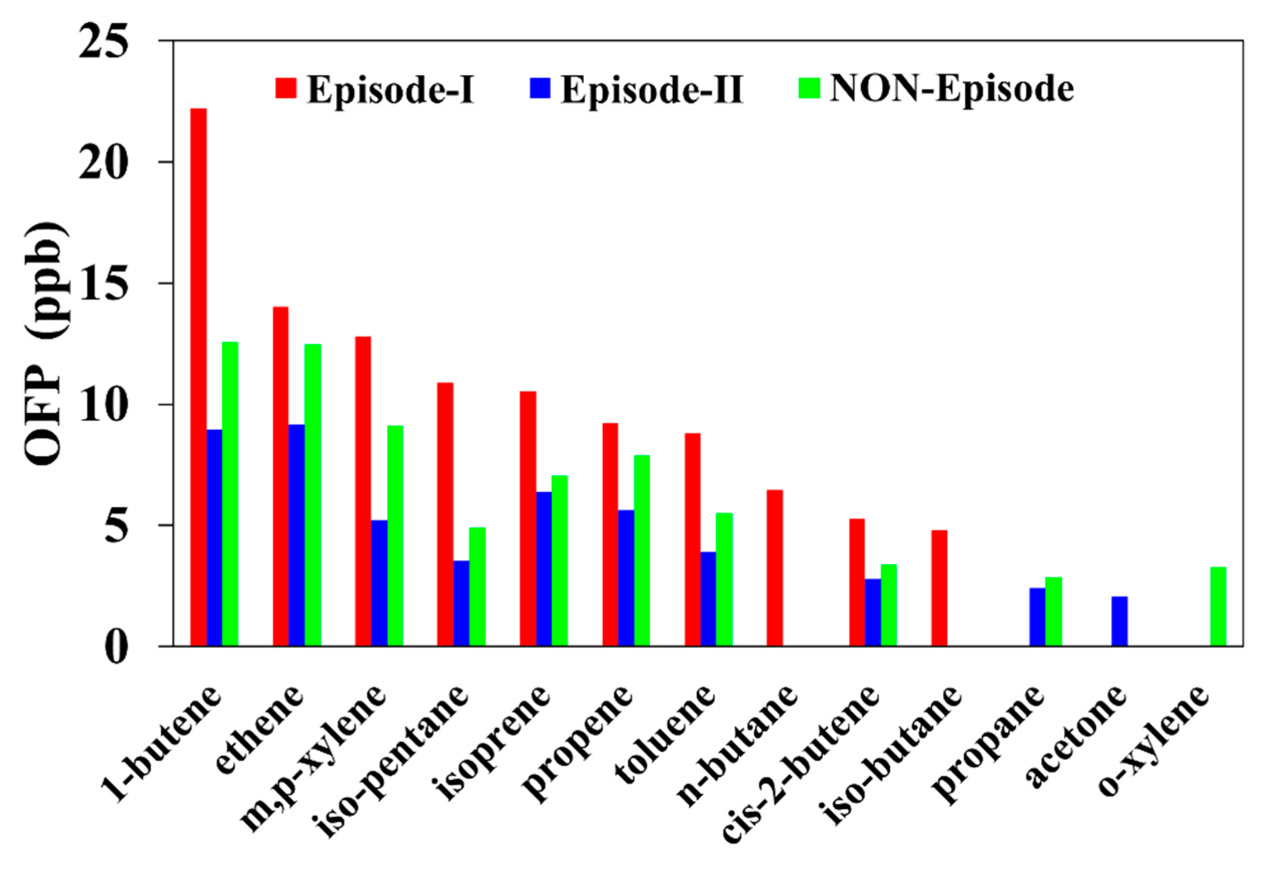
3.4.1. Reactive Species of VOCs

The concentrations of VOCs, OFP and their major group contributions during the O3 and non-O3 episodes are shown in Figure 5. As described above, the highest concentrations of VOCs were found in Episode Ⅰ, followed by the non-O3 episode and Episode Ⅱ. The top three contributors to the concentrations of total VOCs (TVOCs) were alkanes, OVOCs and halocarbons during all events, followed by alkenes and aromatics. The contributions of alkanes, OVOCs and halocarbons to TVOCs were comparable between Episode Ⅰ and non-O3 episode, with 47%, 20% and 17% during Episode Ⅰ, and 45%, 20% and 16% during the non-O3 episode, respectively. In contrast, the proportion of alkanes decreased in Episode Ⅱ, while the contribution of OVOCs was increased by 31% and 35% compared to Episode Ⅰ and non-O3 episode, respectively. It was assumed that the high percentage of OVOCs in Episode Ⅱ was influenced by the regional transmission of surrounding areas, in addition to secondary generation through photochemical oxidation of precursors.
Consistent with the TVOCs, the OFP’s order was as follows: Episode Ⅰ > non-O3 Episode > Episode Ⅱ. Among all events, the primary contributors to OFP were alkenes (43–49%), followed by aromatic hydrocarbons (23–25%) or alkanes (20–27%). It should be noted that alkene concentrations were much lower than those of alkane’s, but the relative contributions to OFP were much higher, which is consistent with previous studies [41,42]. This was attributed to the higher photochemical reaction reactivity of alkenes. Therefore, controlling the emissions of alkenes is an efficient way to reduce the O3 production in the urban area of Jinan.
The comparison of the 10 VOC species that contributed most to OFP during different periods is shown in Figure 6. The OFP of these 10 VOCs contributed 60–66% of the total OFP, whereas 1-butene and ethene were the top two species in all episodes, covering 23–24% of the total OFP. The major OFP contributors were similar for both O3 and non-O3 episodes, including 1-butene, ethene, m/p-xylene, iso-pentane, isoprene, propene and toluene, although they were ranked in a different order.

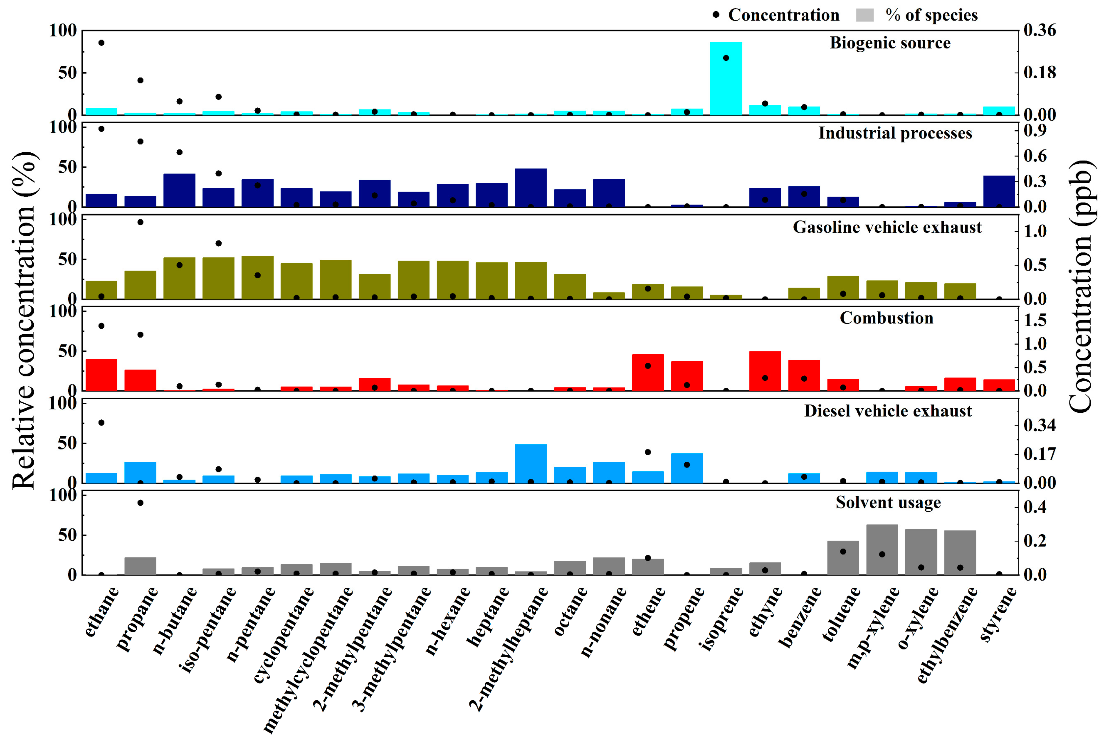
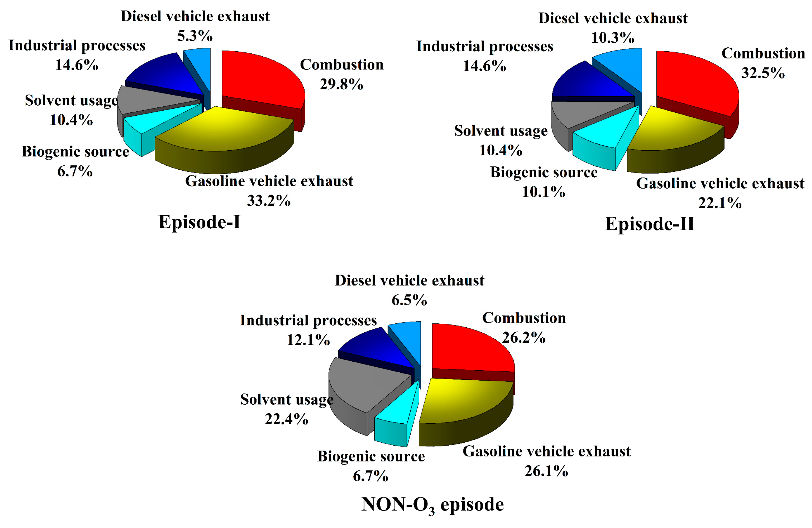
3.4.2. Sources of VOCs Identified via PMF

In this study, six factors were resolved with the PMF model, including gasoline vehicle exhausts, industrial processes, solvent usage, biogenic sources, combustion and diesel vehicle exhausts. Figure 7 displays the source profiles of VOCs and the contributions of individual species to the identified sources.
Factor 1 was dominated by isoprene (86.1%), a typical marker of plant emissions, which could be considered as a biogenic source. Factor 2 was attributed to an industrial source, since it was characterized by high concentrations of styrene (39.1%) and benzene (25.8%), both of which are commonly released by the petrochemical industry [43]. Factor 3 was characterized by a high percentage of low-carbon alkanes, such as iso-pentane (52%) and n-butane (52.1%), as well as n-pentane (54.2%), which are all associated with gasoline vehicle exhaust emissions according to previous studies [44,45]. Factor 3 contributed to low carbon alkenes such as ethylene (18.8%) and propylene (15.8%), indicating that this source is associated with gasoline vehicle exhausts.
Factor 4 was recognized by high concentrations of acetylene (49.7%), ethylene (45.7%) and ethane (39.5%). Acetylene is a well-known tracer for combustion sources, and ethane is commonly associated with natural gas use [46]. Coal and biomass combustion can release significant amounts of ethylene and acetylene [46]. Therefore, factor 4 was identified as combustion sources. Factor 5 was characterized by high contributions of 2-methyl heptane (48%), nonane (26%) and octane (20.1%), as well as benzene, m/p-xylene and other benzene species. Studies have suggested that high-carbon alkanes (C8 or higher) can be considered as exhaust tracers for diesel vehicles [47,48]. Therefore, factor 5 can be considered as a diesel vehicle exhaust source. m,p-Xylene (63.1%) and o-xylene (57.2%) were the dominant species in factor 6. Previous studies have demonstrated that C8–C9 aromatics are strongly associated with the usage of paints and coatings [49]. Thus, factor 6 may be attributed to solvent usage.
Figure 8 shows the contribution of different sources to the measured VOCs for different O3 pollution events. Combustion sources and gasoline vehicle emissions were the dominant sources of VOCs throughout the observation period, contributing to 52–63% of the VOCs. The contribution of solvent usage to VOCs was 12% higher during the non-O3 episode, probably due to the fact that solvent usage sources emitted mainly aromatic hydrocarbons with a relatively higher photochemical reactivity, and the higher temperature and lower humidity during Episodes Ⅰ and Ⅱ favored the rapid photochemical consumption of aromatic hydrocarbons. In contrast, combustion sources and gasoline vehicle exhausts predominantly emit low-carbon alkanes with relatively lower photochemical reactivities, resulting in higher contributions of VOCs from these sources during periods of excess O3 pollution. It is noteworthy that the contribution from gasoline vehicle exhausts was slightly lower during Episode II than the non-O3 episode, which may be related to the fact that this period was mainly concentrated during weekends with a significant decrease in motor vehicle activities, which is consistent with the lower NOX concentration in Episode II in Section 3.1.2. In conclusion, the use of solvents should be controlled in the future to mitigate ozone pollution, and combustion sources and vehicle emissions could be controlled to effectively reduce the concentration levels of VOCs.

3.5. Impact of Air Mass Transport on Different O3 Pollution Episodes

To investigate the influence of regional transport on O3 pollution in Jinan, 24 h backward trajectory simulations were conducted for three different ozone episodes. The four clusters of air masses obtained from the backward trajectory analysis are shown in Figure 9. For Episode Ⅰ, more than 90% of the air masses originated from the south, with 36.11% and 27.08% from the southwest and 29.86% from the southeast. In Episode II, the air masses were also primarily from the south, which was consistent with the monitored wind directions in Section 3.1.1, with 72.5% of air masses from the south (16.67%, 18.33% and 37.50%, respectively) and 27.50% from the east. In the non-O3 episode, air masses from the four directions were more balanced, including east (24.17%), west (23.33%), southeast (35.83%) and north (16.67%). By analyzing the trajectories of air masses transported during different ozone pollution episodes, we found that Jinan City was more likely to suffer O3 pollution in June when the air masses came from the south. The potential sources of O3 in Jinan mainly come from short-range transport from cities in southern Shandong Province and long-range transport from Henan and Anhui Provinces, which have well-developed manufacturing industries, high traffic flow, and high levels of anthropogenic pollutant emissions.

4. Conclusions

Based on continuous measurements of VOCs, trace gases and meteorological parameter s in the urban area of Jinan in June 2021, the characteristics and causes of changes in O3 pollution were explored. The results indicated that high concentrations of ozone precursors and regional transport are the main influencing factors to induce ozone pollution. In addition, meteorological parameters including high temperature and low relative humidity also contribute to ozone generation.
The whole observation was divided into O3 pollution days and non-O3 pollution days according to the China Ambient Air Quality Standards, and the O3 pollution days were categorized into O3 Episode I and O3 Episode II based on the differences in precursor concentrations. The average concentrations of O3 in Episode Ⅰ and Episode Ⅱ were 145.4 μg/m3 and 166.4 μg/m3, respectively, which were 1.6 and 1.8 times higher than those in non-O3 episode (90 μg/m3). During O3 Episode Ⅰ, VOCs and NOX concentrations were 37.1 ppb and 36.3 μg/m3 while the values in the non-O3 episode were 25.0 ppb and 27.1 μg/m3, approximately 48% and 34% higher than those during non-O3 episode. In contrast, the VOCs and NOX decreased by 21% and 27% in Episode Ⅱ compared to non-O3 episode days.
By analyzing the ratios of X/E, we found that the aging level of the air masses in Episode II was significantly higher than those in other episodes. The highest degree of air mass aging in Episode II could not be explained by local photochemical depletion of VOCs as indicated by the daily variations of X/E and OH exposure, and we presumed that the occurrence of high O3 pollution with low O3 precursor concentrations in Episode II can be attributed to the regional transport of the air mass. Differently, O3 pollution in Episode I was dominated by local formation, high concentration of O3 precursors, high temperature and low relative humidity favoring the generation of O3 in Episode I.
The ratios of VOCs/NOX indicating that the formation of O3 in urban Jinan was co-limited by both VOCs and NOX. Six factors were identified by PMF model, including gasoline vehicle exhaust, industrial processes, solvent usage, biogenic source, combustion, and diesel vehicle exhaust. Among them, combustion (26–32%) and gasoline vehicle emissions (22–33%) were the dominant sources of VOCs for the three episodes. Therefore, fuel combustion and vehicle emissions could be controlled to effectively reduce the concentration levels of VOCs in Jinan.
Backward trajectory simulations demonstrated that Jinan City was more likely to suffer O3 pollution in June when the air masses came from the south. In conclusion, in order to effectively mitigate ozone pollution in Jinan, it is necessary to strengthen joint control with neighboring cities, especially those in the south, in addition to reducing local ozone precursor emissions.

Supplementary Materials

The following supporting information can be downloaded at: https://www.mdpi.com/article/10.3390/atmos15020232/s1, Figure S1: Location of the sampling site in this study.

Author Contributions

Conceptualization, B.W.; methodology, C.W.; validation, Y.S. and R.Z.; formal analysis, Y.S.; investigation, Z.L., C.Z., G.F. and X.S.; data curation, H.X., Z.L., N.Y. and Z.X.; writing—original draft preparation, Y.S. and R.Z.; writing—review and editing, B.W. and C.W.; visualization, L.S., G.Y. and R.Z.; supervision, Z.Z., G.P. and C.X.; funding acquisition, B.W. and C.X. All authors have read and agreed to the published version of the manuscript.

Funding

This research was supported by the National Natural Science Foundation of China (41905111), the Shandong Provincial Natural Science Foundation (ZR2019BD030), the National Natural Science Foundation of China (42105104), the Basic Research Program for Integration Pilot of Science, Education and Industry of Qilu University of Technology (Shandong Academy of Science) (2023PY041, 2023PY005, 2023PX096), Qilu University of Technology (Shandong Academy of Science) Talent Research Project (2023RCKY107) and the Major Innovation Projects of Science, Education and Industry Integration of Qilu University of Technology (Shandong Academy of Science) (2022JBZ02-05).

Institutional Review Board Statement

Not applicable.

Informed Consent Statement

Not applicable.

Data Availability Statement

The data presented in this study are available upon request from the corresponding author. The data are not publicly available due to privacy reasons. The data will be used for further research.

Conflicts of Interest

The authors declare no conflicts of interest.

References

  1. Greenstone, M.; He, G.J.; Li, S.J.; Zou, E.Y. China’s War on Pollution: Evidence from the First 5 Years. Rev. Environ. Econ. Policy 2021, 15, 281–299. [Google Scholar] [CrossRef]
  2. Zheng, S.Q.; Kahn, M.E. A New Era of Pollution Progress in Urban China? J. Econ. Perspect. 2017, 31, 71–92. [Google Scholar] [CrossRef]
  3. Liu, Y.M.; Wang, T. Worsening urban ozone pollution in China from 2013 to 2017—Part 2: The effects of emission changes and implications for multi-pollutant control. Atmos. Chem. Phys. 2020, 20, 6323–6337. [Google Scholar] [CrossRef]
  4. Sun, J.; Duan, S.X.; Wang, B.L.; Sun, L.; Zhu, C.Y.; Fan, G.L.; Sun, X.Y.; Xia, Z.Y.; Lv, B.; Yang, J.Y.; et al. Long-Term Variations of Meteorological and Precursor Influences on Ground Ozone Concentrations in Jinan, North China Plain, from 2010 to 2020. Atmosphere 2022, 13, 15. [Google Scholar] [CrossRef]
  5. Xiao, Q.Y.; Geng, G.N.; Xue, T.; Liu, S.G.; Cai, C.L.; He, K.B.; Zhang, Q. Tracking PM2.5 and O3 Pollution and the Related Health Burden in China 2013–2020. Environ. Sci. Technol. 2022, 56, 6922–6932. [Google Scholar] [CrossRef] [PubMed]
  6. Martin, R.V.; Fiore, A.M.; Van Donkelaar, A. Space-based diagnosis of surface ozone sensitivity to anthropogenic emissions. Geophys. Res. Lett. 2004, 31, 4. [Google Scholar] [CrossRef]
  7. Chen, X.Y.; Liu, Y.M.; Lai, A.Q.; Han, S.S.; Fan, Q.; Wang, X.M.; Ling, Z.H.; Huang, F.X.; Fan, S.J. Factors dominating 3-dimensional ozone distribution tropospheric ozone period. Environ. Pollut. 2018, 232, 55–64. [Google Scholar] [CrossRef] [PubMed]
  8. Chen, Z.Y.; Li, R.Y.; Chen, D.L.; Zhuang, Y.; Gao, B.B.; Yang, L.; Li, M.C. Understanding the causal influence of major meteorological factors on ground ozone concentrations across China. J. Clean. Prod. 2020, 242, 118498. [Google Scholar] [CrossRef]
  9. Shen, L.J.; Liu, J.N.; Zhao, T.L.; Xu, X.D.; Han, H.; Wang, H.L.; Shu, Z.Z. Atmospheric transport drives regional interactions of ozone pollution in China. Sci. Total Environ. 2022, 830, 154634. [Google Scholar] [CrossRef] [PubMed]
  10. Wang, D.C.; Zhou, J.B.; Han, L.; Tian, W.A.; Wang, C.H.; Li, Y.J.; Chen, J.H. Source apportionment of VOCs and ozone formation potential and transport in Chengdu, China. Atmos. Pollut. Res. 2023, 14, 101730. [Google Scholar] [CrossRef]
  11. Guan, Y.A.; Liu, X.J.; Zheng, Z.Y.; Dai, Y.W.; Du, G.M.; Han, J.; Hou, L.A.; Duan, E.R. Summer O3 pollution cycle characteristics and VOCs sources in a central city of Beijing-Tianjin-Hebei area, China. Environ. Pollut. 2023, 323, 7. [Google Scholar] [CrossRef] [PubMed]
  12. Xiao, C.C.; Chang, M.; Guo, P.K.; Gu, M.F.; Li, Y. Analysis of air quality characteristics of Beijing-Tianjin-Hebei and its surrounding air pollution transport channel cities in China. J. Environ. Sci. 2020, 87, 213–227. [Google Scholar] [CrossRef]
  13. Xu, J.; Li, J.; Zhao, X.J.; Zhang, Z.Y.; Pan, Y.B.; Li, Q.C. Effectiveness of emission control in sensitive emission regions associated with local atmospheric circulation in O3 pollution reduction: A case study in the Beijing-Tianjin-Hebei region. Atmos. Environ. 2022, 269, 13. [Google Scholar] [CrossRef]
  14. Li, L.; An, J.Y.; Huang, L.; Yan, R.S.; Huang, C.; Yarwood, R. Ozone source apportionment over the Yangtze River Delta region, China: Investigation of regional transport, sectoral contributions and seasonal differences. Atmos. Environ. 2019, 202, 269–280. [Google Scholar] [CrossRef]
  15. Liu, Y.; Li, L.; An, J.Y.; Huang, L.; Yan, R.S.; Huang, C.; Wang, H.L.; Wang, Q.; Wang, M.; Zhang, W. Estimation of biogenic VOC emissions and its impact on ozone formation over the Yangtze River Delta region, China. Atmos. Environ. 2018, 186, 113–128. [Google Scholar] [CrossRef]
  16. Liu, X.F.; Wang, N.; Lyu, X.P.; Zeren, Y.Z.; Jiang, F.; Wang, X.M.; Zou, S.C.; Ling, Z.H.; Guo, H. Photochemistry of ozone pollution in autumn in Pearl River Estuary, South China. Sci. Total Environ. 2021, 754, 141812. [Google Scholar] [CrossRef] [PubMed]
  17. Ou, J.M.; Zheng, J.Y.; Li, R.R.; Huang, X.B.; Zhong, Z.M.; Zhong, L.J.; Lin, H. Speciated OVOC and VOC emission inventories and their implications for reactivity-based ozone control strategy in the Pearl River Delta region, China. Sci. Total Environ. 2015, 530, 393–402. [Google Scholar] [CrossRef]
  18. Wang, M.; Zeng, L.M.; Lu, S.H.; Shao, M.; Liu, X.L.; Yu, X.N.; Chen, W.T.; Yuan, B.; Zhang, Q.; Hu, M.; et al. Development and validation of a cryogen-free automatic gas chromatograph system (GC-MS/FID) for online measurements of volatile organic compounds. Anal. Methods 2014, 6, 9424–9434. [Google Scholar] [CrossRef]
  19. Carter, W.P.L. Development of the SAPRC-07 chemical mechanism. Atmos. Environ. 2010, 44, 5324–5335. [Google Scholar] [CrossRef]
  20. Luo, H.; Li, G.Y.; Chen, J.Y.; Lin, Q.H.; Ma, S.T.; Wang, Y.J.; An, T.C. Spatial and temporal distribution characteristics and ozone formation potentials of volatile organic compounds from three typical functional areas in China. Environ. Res. 2020, 183, 109141. [Google Scholar] [CrossRef]
  21. Han, C.; Liu, R.R.; Luo, H.; Li, G.Y.; Ma, S.T.; Chen, J.Y.; An, T.C. Pollution profiles of volatile organic compounds from different urban functional areas in Guangzhou China based on GC/MS and PTR-TOF-MS: Atmospheric environmental implications. Atmos. Environ. 2019, 214, 116843. [Google Scholar] [CrossRef]
  22. Jimenez, J.L.; Canagaratna, M.R.; Donahue, N.M.; Prevot, A.S.H.; Zhang, Q.; Kroll, J.H.; DeCarlo, P.F.; Allan, J.D.; Coe, H.; Ng, N.L.; et al. Evolution of Organic Aerosols in the Atmosphere. Science 2009, 326, 1525–1529. [Google Scholar] [CrossRef]
  23. Song, M.D.; Li, X.; Yang, S.D.; Yu, X.N.; Zhou, S.X.; Yang, Y.M.; Chen, S.Y.; Dong, H.B.; Liao, K.R.; Chen, Q.; et al. Spatiotemporal variation, sources, and secondary transformation potential of volatile organic compounds in Xi’an, China. Atmos. Chem. Phys. 2021, 21, 4939–4958. [Google Scholar] [CrossRef]
  24. Wu, Y.J.; Fan, X.L.; Liu, Y.; Zhang, J.Q.; Wang, H.; Sun, L.A.; Fang, T.E.; Mao, H.J.; Hu, J.; Wu, L.; et al. Source apportionment of VOCs based on photochemical loss in summer at a suburban site in Beijing. Atmos. Environ. 2023, 293, 119459. [Google Scholar] [CrossRef]
  25. Li, Y.S.; Liu, Y.; Hou, M.; Huang, H.M.; Fan, L.Y.; Ye, D.Q. Characteristics and sources of volatile organic compounds (VOCs) in Xinxiang, China, during the 2021 summer ozone pollution control. Sci. Total Environ. 2022, 842, 11. [Google Scholar] [CrossRef] [PubMed]
  26. Liu, C.T.; Zhang, C.L.; Liu, J.F.; Liu, P.F.; Mu, Y.J. Characteristics and sources of volatile organic compounds during summertime in Tai’an, China. Atmos. Pollut. Res. 2022, 13, 101340. [Google Scholar] [CrossRef]
  27. Yang, X.Y.; Wu, K.; Wang, H.L.; Liu, Y.M.; Gu, S.; Lu, Y.Q.; Zhang, X.L.; Hu, Y.S.; Ou, Y.H.; Wang, S.G.; et al. Summertime ozone pollution in Sichuan Basin, China: Meteorological conditions, sources and process analysis. Atmos. Environ. 2020, 226, 12. [Google Scholar] [CrossRef]
  28. Wang, B.L.; Liu, Z.G.; Li, Z.; Sun, Y.C.; Wang, C.; Zhu, C.Y.; Sun, L.; Yang, N.; Bai, G.; Fan, G.L.; et al. Characteristics, chemical transformation and source apportionment of volatile organic compounds (VOCs) during wintertime at a suburban site in a provincial capital city, east China. Atmos. Environ. 2023, 298, 11. [Google Scholar] [CrossRef]
  29. Sun, X.-Y.; Zhao, M.; Shen, H.-Q.; Liu, Y.; Du, M.-Y.; Zhang, W.-J.; Xu, H.-Y.; Fan, G.-L.; Gong, H.-L.; Li, Q.-S.J.H.J.k.X.H.K. Ozone Formation and Key VOCs of a Continuous Summertime O 3 Pollution Event in Ji’nan. Atmos. Chem. Phys. 2022, 43, 686–695. [Google Scholar] [CrossRef]
  30. Shao, M.; Wang, B.; Lu, S.H.; Yuan, B.; Wang, M. Effects of Beijing Olympics Control Measures on Reducing Reactive Hydrocarbon Species. Environ. Sci. Technol. 2011, 45, 514–519. [Google Scholar] [CrossRef]
  31. Atkinson, R.; Arey, J.J.C. Atmospheric Degradation of Volatile Organic Compounds. Chem. Rev. 2004, 35, 4605–4638. [Google Scholar] [CrossRef]
  32. Fu, J.S.; Dong, X.Y.; Gao, Y.; Wong, D.C.; Lam, Y.F. Sensitivity and linearity analysis of ozone in East Asia: The effects of domestic emission and intercontinental transport. J. Air Waste Manage. Assoc. 2012, 62, 1102–1114. [Google Scholar] [CrossRef] [PubMed]
  33. Lin, X.; Trainer, M.; Liu, S.C. On the nonlinearity of the tropospheric ozone production. J. Geophys. Res. Atmos. 1988, 93, 15879–15888. [Google Scholar] [CrossRef]
  34. Yang, Y.C.; Liu, X.G.; Zheng, J.; Tan, Q.W.; Feng, M.; Qu, Y.; An, J.L.; Cheng, N.L. Characteristics of one-year observation of VOCs, NOx, and O3 at an urban site in Wuhan, China. J. Environ. Sci. 2019, 79, 297–310. [Google Scholar] [CrossRef]
  35. Ren, X.; Wen, Y.P.; He, Q.S.; Cui, Y.; Gao, X.Y.; Li, F.; Wang, Y.H.; Guo, L.L.; Li, H.Y.; Wang, X.M. Higher contribution of coking sources to ozone formation potential from volatile organic compounds in summer in Taiyuan, China. Atmos. Pollut. Res. 2021, 12, 101083. [Google Scholar] [CrossRef]
  36. Seinfeld, J.H. Urban Air Pollution: State of the Science. Science 1989, 243, 745–752. [Google Scholar] [CrossRef] [PubMed]
  37. Li, K.; Chen, L.H.; Ying, F.; White, S.J.; Jang, C.; Wu, X.C.; Gao, X.; Hong, S.M.; Shen, J.D.; Azzi, M.; et al. Meteorological and chemical impacts on ozone formation: A case study in Hangzhou, China. Atmos. Res. 2017, 196, 40–52. [Google Scholar] [CrossRef]
  38. Li, Y.S.; Yin, S.S.; Yu, S.J.; Bai, L.; Wang, X.D.; Lu, X.; Ma, S.L. Characteristics of ozone pollution and the sensitivity to precursors during early summer in central plain, China. J. Environ. Sci. 2021, 99, 354–368. [Google Scholar] [CrossRef]
  39. Li, L.; Xie, F.J.; Li, J.Y.; Gong, K.J.; Xie, X.D.; Qin, Y.; Qin, M.M.; Hu, J.L. Diagnostic analysis of regional ozone pollution in Yangtze River Delta, China: A case study in summer 2020. Sci. Total Environ. 2022, 812, 151511. [Google Scholar] [CrossRef]
  40. Gong, S.; Zhang, L.; Liu, C.; Lu, S.; Pan, W.; Zhang, Y. Multi-scale analysis of the impacts of meteorology and emissions on PM2.5 and O3 trends at various regions in China from 2013 to 2020 2. Key weather elements and emissions. Sci. Total Environ. 2022, 824, 153847. [Google Scholar] [CrossRef]
  41. Zhang, Y.C.; Li, R.; Fu, H.B.; Zhou, D.; Chen, J.M. Observation and analysis of atmospheric volatile organic compounds in a typical petrochemical area in Yangtze River Delta, China. J. Environ. Sci. 2018, 71, 233–248. [Google Scholar] [CrossRef]
  42. Zhou, M.M.; Jiang, W.; Gao, W.D.; Zhou, B.H.; Liao, X.C. A high spatiotemporal resolution anthropogenic VOC emission inventory for Qingdao City in 2016 and its ozone formation potential analysis. Process Saf. Environ. Prot. 2020, 139, 147–160. [Google Scholar] [CrossRef]
  43. Zhang, C.; Liu, X.G.; Zhang, Y.Y.; Tan, Q.W.; Feng, M.; Qu, Y.; An, J.L.; Deng, Y.J.; Zhai, R.X.; Wang, Z.; et al. Characteristics, source apportionment and chemical conversions of VOCs based on a comprehensive summer observation experiment in Beijing. Atmos. Pollut. Res. 2021, 12, 183–194. [Google Scholar] [CrossRef]
  44. Liu, P.-W.G.; Yao, Y.-C.; Tsai, J.-H.; Hsu, Y.-C.; Chang, L.-P.; Chang, K.-H. Source impacts by volatile organic compounds in an industrial city of southern Taiwan. Sci. Total Environ. 2008, 398, 154–163. [Google Scholar] [CrossRef] [PubMed]
  45. Watson, J.G.; Chow, J.C.; Fujita, E.M. Review of volatile organic compound source apportionment by chemical mass balance. Atmos. Environ. 2001, 35, 1567–1584. [Google Scholar] [CrossRef]
  46. Xiong, Y.; Du, K. Source-resolved attribution of ground-level ozone formation potential from VOC emissions in Metropolitan Vancouver, BC. Sci. Total Environ. 2020, 721, 137698. [Google Scholar] [CrossRef] [PubMed]
  47. Fang, H.; Luo, S.L.; Huang, X.Q.; Fu, X.W.; Xiao, S.X.; Zeng, J.Q.; Wang, J.; Zhang, Y.L.; Wang, X.M. Ambient naphthalene and methylnaphthalenes observed at an urban site in the Pearl River Delta region: Sources and contributions to secondary organic aerosol. Atmos. Environ. 2021, 252, 118295. [Google Scholar] [CrossRef]
  48. Wang, W.J.; Fang, H.; Zhang, Y.; Ding, Y.Y.; Hua, F.; Wu, T.; Yan, Y.Z. Characterizing sources and ozone formations of summertime volatile organic compounds observed in a medium-sized city in Yangtze River Delta region. Chemosphere 2023, 328, 138609. [Google Scholar] [CrossRef] [PubMed]
  49. Liu, Y.; Shao, M.; Fu, L.; Lu, S.; Zeng, L.; Tang, D. Source profiles of volatile organic compounds (VOCs) measured in China: Part I. Atmos. Environ. 2008, 42, 6247–6260. [Google Scholar] [CrossRef]
Figure 1. Time series of O3, VOCs, NOX and meteorological parameters during the campaign.
Atmosphere 15 00232 g001
Figure 2. Diurnal variations of meteorological parameters, O3 and its precursors during different O3 episodes.
Atmosphere 15 00232 g002
Figure 3. Diurnal variations of X/E and OH exposure. The red dashed lines represent the initial emission ratio of X/E.
Atmosphere 15 00232 g003
Figure 4. Correlations of VOCs and NOX during different episodes in Jinan.
Atmosphere 15 00232 g004
Figure 5. Concentrations of VOCs, OFP and their major group contributions during different O3 episodes.
Atmosphere 15 00232 g005
Figure 6. Top 10 species that contributed to OFP during different periods.
Atmosphere 15 00232 g006
Figure 7. Source profiles resolved with PMF.
Atmosphere 15 00232 g007
Figure 8. The contributions of six sources to the measured VOC concentrations during different events.
Atmosphere 15 00232 g008
Figure 9. Backward trajectory analysis during the observation in the study area.
Atmosphere 15 00232 g009
Table 1. The average trace gas concentrations and meteorological parameters during different ozone episodes in June 2021.
O3
μg/m3
VOCs
ppb
NO2
μg/m3
NOx
μg/m3
WS
m/s
RH
%
T
°C
EP I145.437.129.436.31.5947.230.5
EP II166.419.814.719.81.6553.530.8
NON-O396.325.020.527.11.5963.426.0
Average136.028.121.527.71.6055.028.9
Disclaimer/Publisher’s Note: The statements, opinions and data contained in all publications are solely those of the individual author(s) and contributor(s) and not of MDPI and/or the editor(s). MDPI and/or the editor(s) disclaim responsibility for any injury to people or property resulting from any ideas, methods, instructions or products referred to in the content.

