

Lightning Risk Warning Method Using Atmospheric Electric Field Based on EEWT-ASG and Morpho

Abstract
:1. Introduction
2. Method
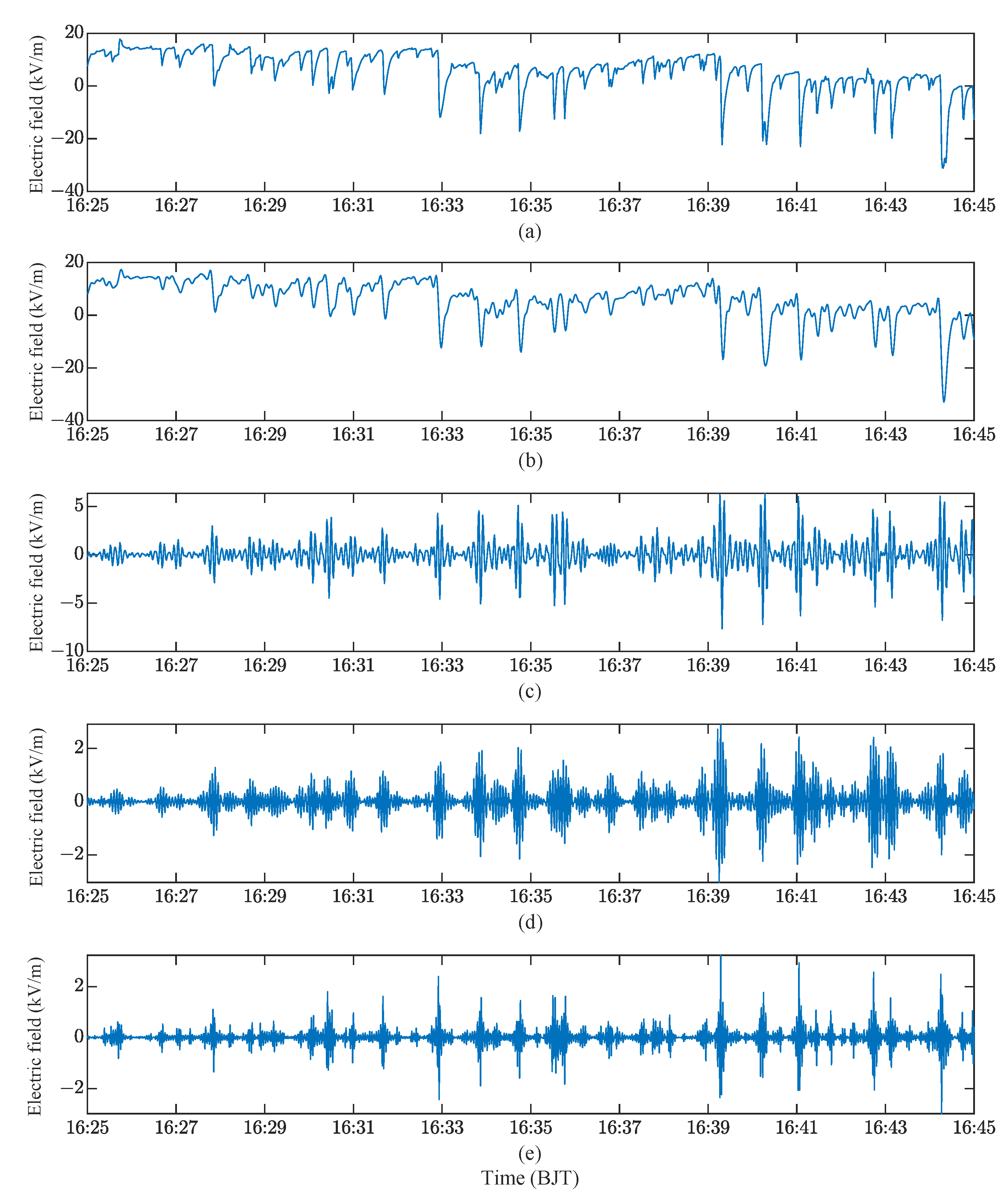
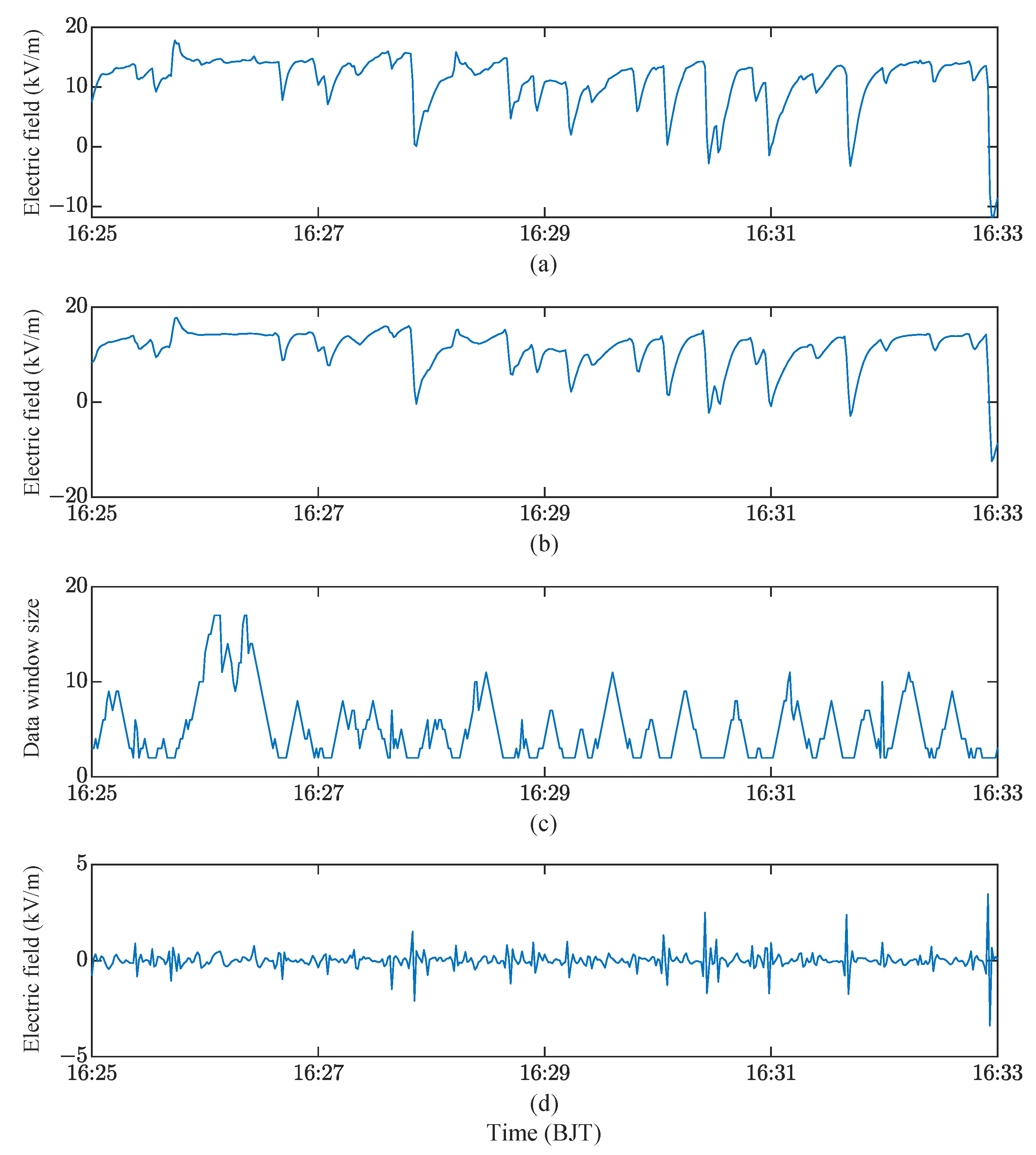
2.1. EEWT-ASG
2.2. Calculation of Global Trend Based on Morpho
- The flat top is classified as the upward region if both the left and right sides of the flat top are within the upward region;
- The flat top is designated as the downward region if both the left and right sides of the flat top are within the downward region;
- The remaining flat tops, identified as the complex region, have their trends disregarded.
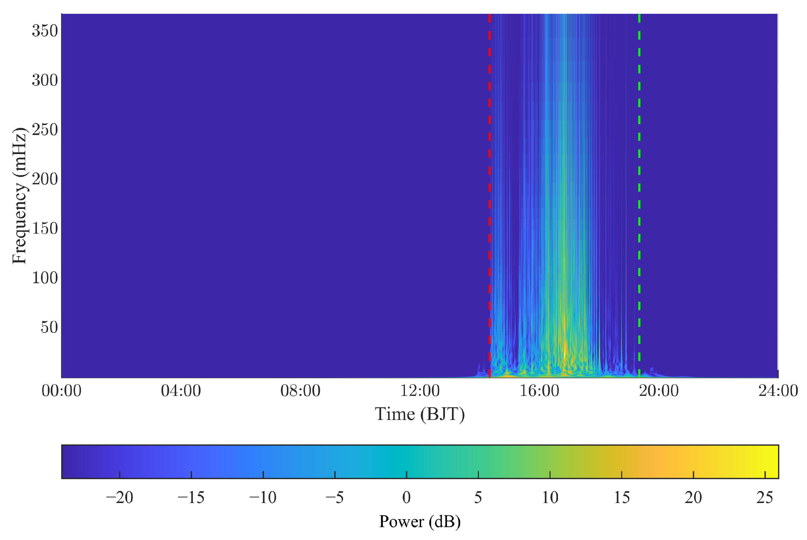
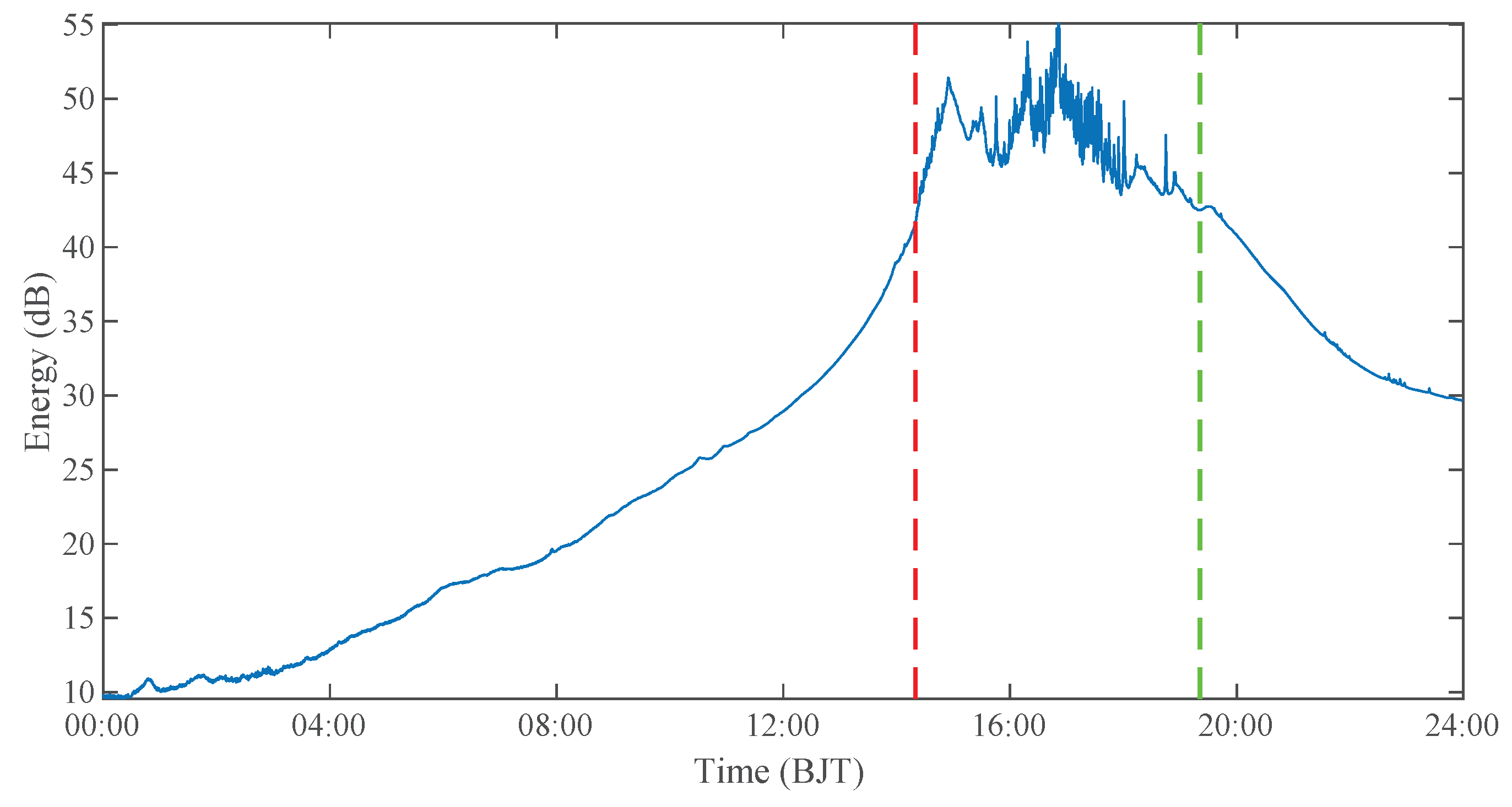
3. Time-Frequency Spectrum Feature Statistics
4. Lightning Risk Warning Method and Evaluation
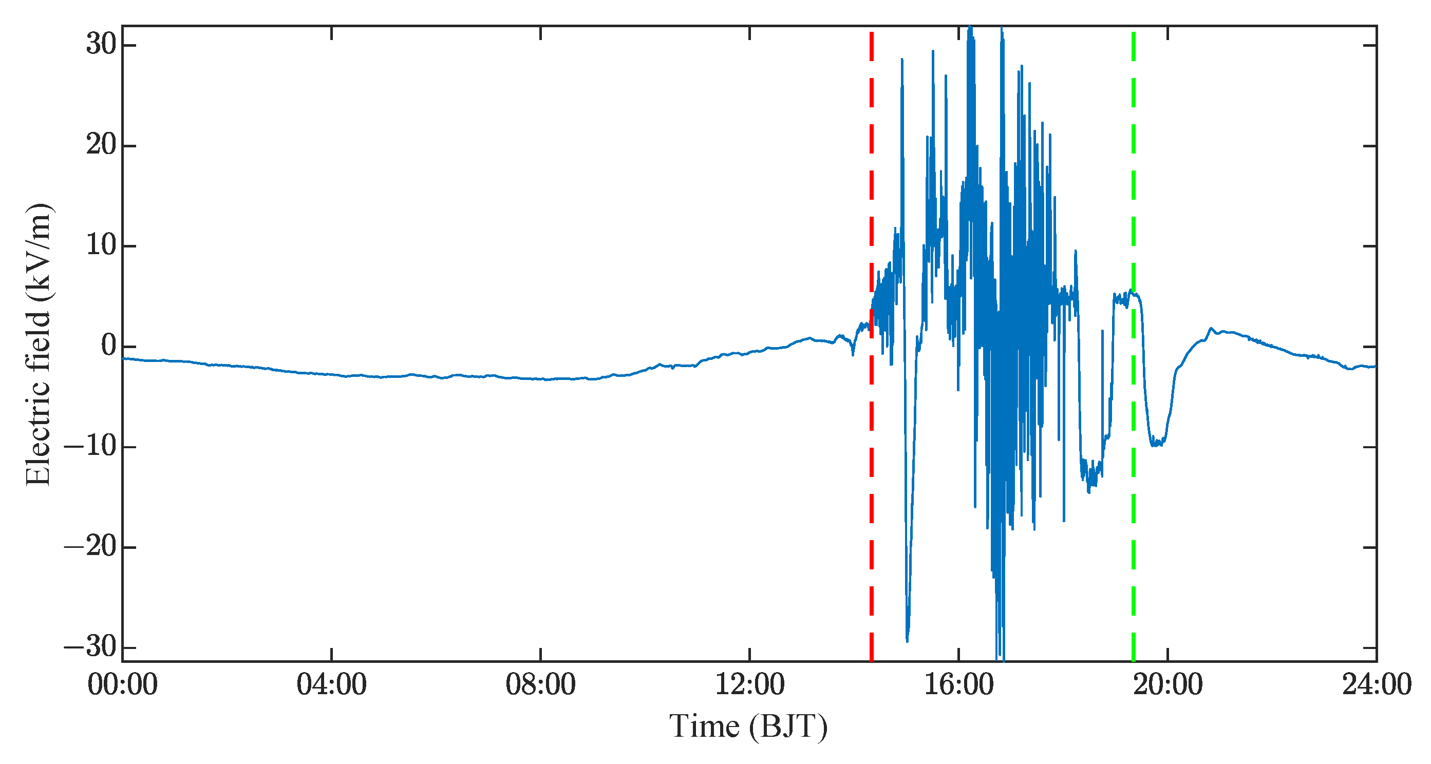
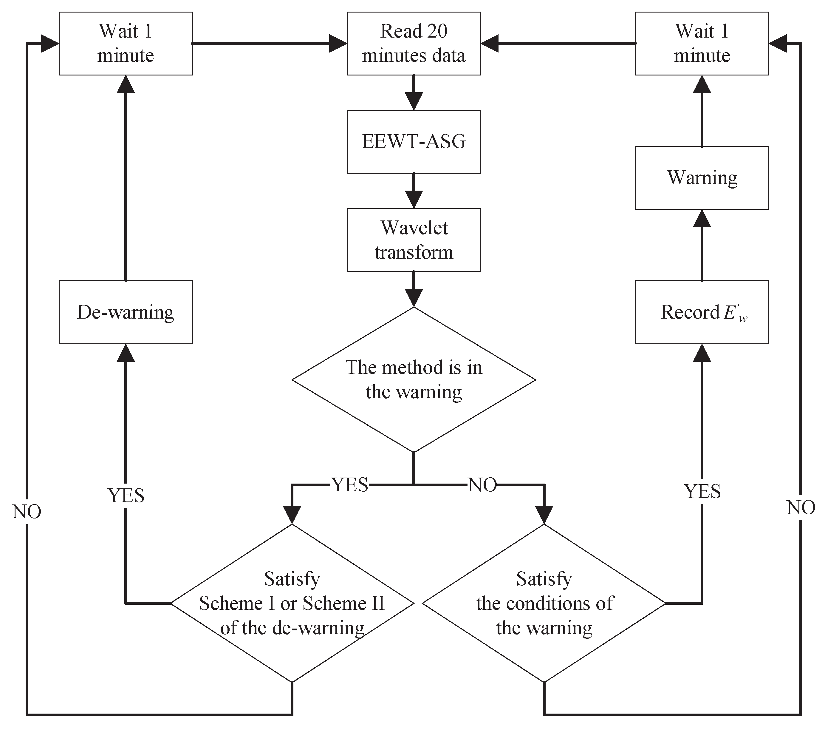
4.1. Lightning Risk Warning Method Based on AEF Signal
- and of the AEF signal show a global upward trend over 20 min;
- > 0.5 mHz, >− 20 dB, and > 0.5 kV/m in 10 min;
- and of the AEF signal show a global downward trend over 20 min;
- ≤ 1 dB and ≤ 1 kV/m in 10 min;
- The sum of the 10 judgments for was less than 0.1 mHz;
- ≤ 1 kV/m in 10 min;
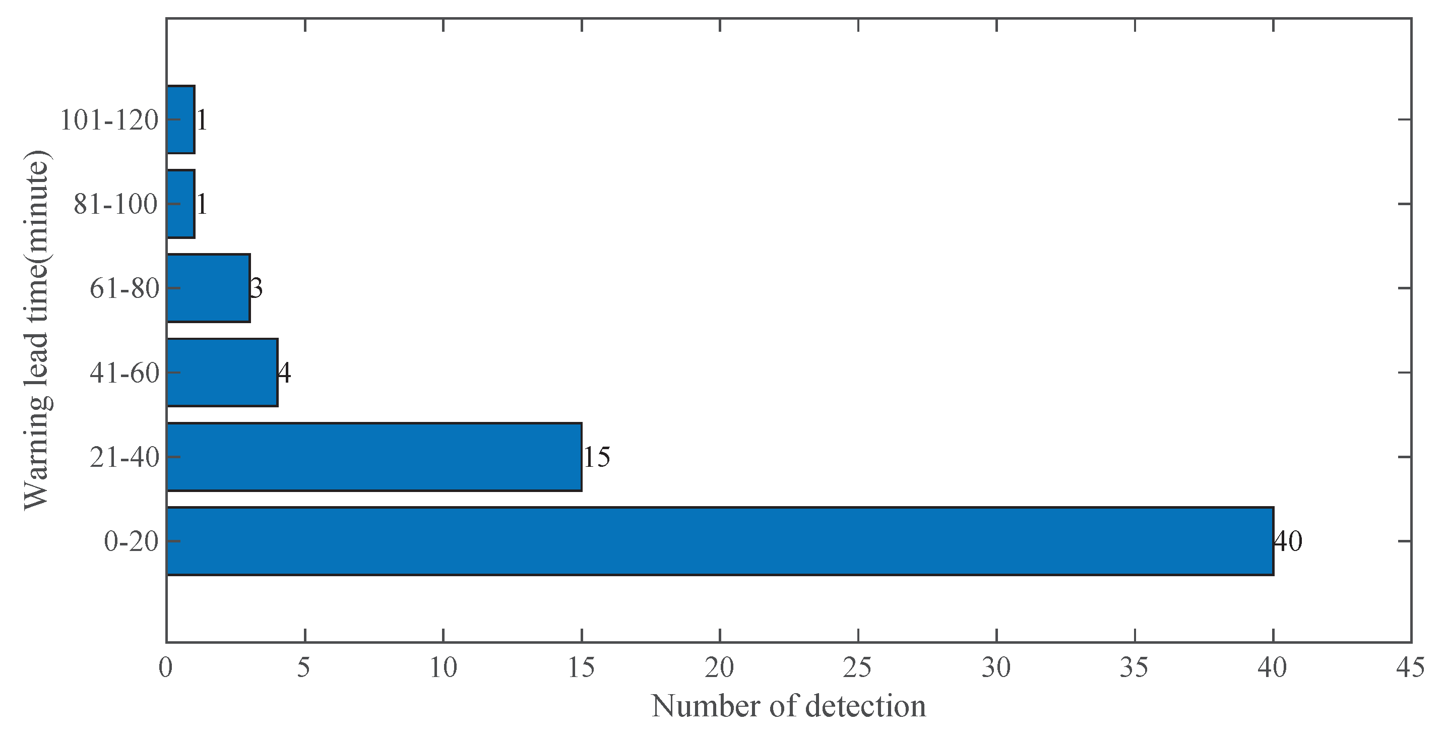
4.2. Evaluation Metrics
4.3. Results and Analysis
5. Discussions and Conclusions
- (1)
- We introduced the EEWT-ASG and morpho-based global trend calculation methods, specifically designed for lightning warning scenarios.
- (2)
- Employing Wavelet Transform (WT), we conducted a statistical analysis of the time-frequency spectral characteristics for both lightning and non-lightning events.
- (3)
- We proposed a lightning risk warning method that utilizes features from both time and frequency domains.
Author Contributions
Funding
Institutional Review Board Statement
Informed Consent Statement
Data Availability Statement
Conflicts of Interest
References
- Holle, R.L. A summary of recent national-scale lightning fatality studies. Weather Clim. Soc. 2016, 8, 35–42. [Google Scholar] [CrossRef]
- Yin, Q.; Liu, H.; Fan, X.; Zhang, Y.; Zhuang, Y.; Wang, F.; Du, H.; Huang, X.; Chen, S.; Chen, L. Lightning fatalities in China, 2009–2018. J. Agric. Meteorol. 2021, 77, 150–159. [Google Scholar]
- Bernard, M.; Underwood, S.J.; Berti, M.; Simoni, A.; Gregoretti, C. Observations of the atmospheric electric field preceding intense rainfall events in the Dolomite Alps near Cortina d’Ampezzo, Italy. Meteorol. Atmos. Phys. 2020, 132, 99–111. [Google Scholar] [CrossRef]
- Odzimek, A.; Baranski, P.; Kubicki, M.; Jasinkiewicz, D. Electrical signatures of Nimbostratus and Stratus clouds in ground-level vertical atmospheric electric field and current density at mid-latitude station Swider, Poland. Atmos. Res. 2018, 209, 188–203. [Google Scholar] [CrossRef]
- Hoeft, R.; Wakefield, C. Evaluation of the electric field mill as an effective and efficient means of lightning detection. In Proceedings of the International Aerospace and Ground Conference on Lightning and Static Electricity, National Interagency Coordinating Group, Atlantic City, NJ, USA, 6–8 October 1992. [Google Scholar]
- Montanya, J.; Bergas, J.; Hermoso, B. Electric field measurements at ground level as a basis for lightning hazard warning. J. Electrost. 2004, 60, 241–246. [Google Scholar] [CrossRef]
- Murphy, M.J.; Holle, R.L.; Demetriades, N.W. Cloud-to-ground lightning warnings using electric field mill and lightning observations. In Proceedings of the 20th International Lightning Detection Conference, Tucson, AZ, USA, 21–23 April 2008; pp. 21–23. [Google Scholar]
- Aranguren, D.; Montanya, J.; Sola, G.; March, V.; Romero, D.; Torres, H. On the lightning hazard warning using electrostatic field: Analysis of summer thunderstorms in Spain. J. Electrost. 2009, 67, 507–512. [Google Scholar] [CrossRef]
- Srivastava, A.; Mishra, M.; Kumar, M. Lightning alarm system using stochastic modelling. Nat. Hazards 2015, 75, 1–11. [Google Scholar] [CrossRef]
- Ying, L.I.; Wang, Z.; Xiao, W.; Zeng, Q.; Yang, T. FFT analysis on atmospheric electric field and the applications in thunderstorm prediction. J. Meteorol. Sci. 2013, 33, 66–70. [Google Scholar]
- Xu, D.; Wang, Z.; Zeng, Q.; Xue, A. EMD Based Analysis of Atmospheric Electric Field Data. Meteorol. Sci. Technol. 2013, 41, 170–176. (In Chinese) [Google Scholar]
- Kang, H.; Liu, C.; Jiang, X. Weather Recognition Algorithm Based on the Characteristics of Atmospheric Electric Field Signal. Comput. Simul. 2014, 31, 312–315. [Google Scholar]
- Lu, Y.; Zhou, Z.; Gu, S.; Wu, D.; Guo, J.; Tao, H. Research on lightning warning method based on the characteristics of atmospheric electric field. In Proceedings of the 2016 33rd International Conference on Lightning Protection (ICLP), Estoril, Portugal, 25–30 September 2016; pp. 1–5. [Google Scholar]
- Yang, X.; Xing, H.; Zhuang, L. A thunderstorm cloud point charge localization method based on CEEMDAN and SG filtering. IEEE Access 2021, 9, 17049–17059. [Google Scholar] [CrossRef]
- Torres, M.E.; Colominas, M.A.; Schlotthauer, G.; Flandrin, P. A complete ensemble empirical mode decomposition with adaptive noise. In Proceedings of the 2011 IEEE International Conference on Acoustics, Speech and Signal Processing (ICASSP), Prague, Czech Republic, 22–27 May 2011; pp. 4144–4147. [Google Scholar]
- Gilles, J. Empirical wavelet transform. IEEE Trans. Signal Process. 2013, 61, 3999–4010. [Google Scholar] [CrossRef]
- Gilles, J.; Heal, K. A parameterless scale-space approach to find meaningful modes in histograms—Application to image and spectrum segmentation. Int. J. Wavelets Multiresolut. Inf. Process. 2014, 12, 1450044. [Google Scholar] [CrossRef]
- Hu, Y.; Li, F.; Li, H.; Liu, C. An enhanced empirical wavelet transform for noisy and non-stationary signal processing. Digit. Signal Process. 2017, 60, 220–229. [Google Scholar] [CrossRef]
- Lee Rodgers, J.; Nicewander, W.A. Thirteen ways to look at the correlation coefficient. Am. Stat. 1988, 42, 59–66. [Google Scholar] [CrossRef]
- John, A.; Sadasivan, J.; Seelamantula, C.S. Adaptive Savitzky-Golay filtering in non-Gaussian noise. IEEE Trans. Signal Process. 2021, 69, 5021–5036. [Google Scholar] [CrossRef]
- Muthusivagami, R. A survey on ECG signal denoising using S-transform and SG filtering. Int. J. Adv. Res. 2020, 8, 332–336. [Google Scholar] [CrossRef]
- Gilles, J.; Tran, G.; Osher, S. 2D empirical transforms. Wavelets, ridgelets, and curvelets revisited. SIAM J. Imaging Sci. 2014, 7, 157–186. [Google Scholar] [CrossRef]
- Yang, P.; Peng, C.; Fang, D.; Wen, X.; Xia, S. Design, fabrication and application of an SOI-based resonant electric field microsensor with coplanar comb-shaped electrodes. J. Micromech. Microeng. 2013, 23, 055002. [Google Scholar] [CrossRef]
- Yang, P.; Chen, B.; Wen, X.; Peng, C.; Xia, S.; Hao, Y. A novel MEMS chip-based atmospheric electric field sensor for lightning hazard warning applications. In Proceedings of the 2015 IEEE SENSORS, Busan, Republic of Korea, 1–4 November 2015; pp. 1–4. [Google Scholar]
- Zhang, Y.; Lu, W.; Chen, L.; Wu, B.; Qi, Q.; Ma, Y.; Zhang, Y.; Zheng, D.; Yan, X.; Meng, Q. Evaluation of GHMLLS Performance Characteristics Based on Observations of Artificially Triggered Lightning. J. Appl. Meteorol. Sci. 2022, 33, 329–340. [Google Scholar]
- Zhou, J.; Zeng, Q.; Shah, A.B.; Jiao, X. A lighting warning algorithm using electric filed mills network and lightning locating system. In Proceedings of the 2016 12th International Conference on Natural Computation, Fuzzy Systems and Knowledge Discovery (ICNC-FSKD), Changsha, China, 13–15 August 2016; pp. 1631–1635. [Google Scholar]
- Li, X.; Hayawi, K.; Chen, Y.; Chang, S.Y.; Wen, H.; Ho, P.H.; Yang, L.; Yin, Q. False Data Injection Attack on Atmospheric Electric Field in Thunderstorm Warning. In Proceedings of the 2022 International Conference on Computing, Communication, Perception and Quantum Technology (CCPQT), Xiamen, China, 5–7 August 2022; pp. 219–223. [Google Scholar]
- Zeng, Q.; Wang, Z.; Guo, F.; Feng, M.; Zhou, S.; Wang, H.; Xu, D. The application of lightning forecasting based on surface electrostatic field observations and radar data. J. Electrost. 2013, 71, 6–13. [Google Scholar] [CrossRef]
- Cooper, M.A.; Holle, R.L. Reducing Lightning Injuries Worldwide; Springer: Berlin/Heidelberg, Germany, 2019. [Google Scholar]


| Category | Phase | Period | Index | Average | Range | |
|---|---|---|---|---|---|---|
| Min | Max | |||||
| Lightning | Warning | Before | 5.51 | 0.02 | 14.46 | |
| 225.54 | 0 | 368.28 | ||||
| 0 | 0 | 0 | ||||
| STD | 1.80 | 0.21 | 6.93 | |||
| After | 7.19 | 0.99 | 14.47 | |||
| 222.83 | 62.65 | 341.84 | ||||
| 0 | 0 | 0 | ||||
| STD | 5.73 | 0.22 | 59.06 | |||
| De-warning | Before | 6.10 | 0.08 | 16.50 | ||
| 212.06 | 13.88 | 368.28 | ||||
| 0 | 0 | 0 | ||||
| STD | 1.55 | 0.22 | 5.88 | |||
| After | 3.79 | 0 | 10.89 | |||
| 137.25 | 0 | 293.49 | ||||
| 0 | 0 | 0 | ||||
| STD | 1.59 | 0.18 | 6.77 | |||
| Non-lightning | 0.01 | 0 | 2.64 | |||
| 0.24 | 0 | 144.30 | ||||
| 0 | 0 | 0 | ||||
| STD | 0.06 | 0.01 | 4.80 | |||
| Filter | No Filter | CEEMDAN-SG | EEWT-ASG | ||||||
|---|---|---|---|---|---|---|---|---|---|
| Index | Average | Range | Average | Range | Average | Range | |||
| 12.96 | 5.33 | 38.08 | 12.23 | 4.07 | 34.94 | 12.48 | 4.07 | 34.97 | |
| 27.89 | 17.01 | 57.07 | 16.14 | 16.14 | 51.82 | 27.82 | 17.79 | 52.20 | |
| 1.91 | 0 | 16.72 | 2.18 | 0 | 17.21 | 2.07 | 0 | 17.48 | |
| 13.54 | 5.89 | 30.82 | 12.77 | 5.11 | 28.87 | 13.8 | 5.52 | 28.40 | |
| 34.36 | 20.98 | 59.54 | 31.95 | 22.23 | 54.56 | 37.39 | 25.06 | 54.77 | |
| 0.75 | 0 | 5.68 | 1.20 | 0 | 8.69 | 1.03 | 0 | 9.13 | |
| Method | Lightning | Non-Lightning | ||||
|---|---|---|---|---|---|---|
| POD | MAR | FAR | CSI | WLT (min) | POD | |
| EFAI [28] | 18.07% | 81.93% | 80.52% | 0.11 | 19.19 | 42.61% |
| EFDI [28] | 91.57% | 8.43% | 60.00% | 0.38 | 32.48 | 80.00% |
| Lu [13] | 18.07% | 81.93% | 70.59% | 0.13 | 10.04 | 98.26% |
| We proposed | 77.11% | 22.89% | 40.19% | 0.51 | 22.27 | 90.24% |
Disclaimer/Publisher’s Note: The statements, opinions and data contained in all publications are solely those of the individual author(s) and contributor(s) and not of MDPI and/or the editor(s). MDPI and/or the editor(s) disclaim responsibility for any injury to people or property resulting from any ideas, methods, instructions or products referred to in the content. |
© 2023 by the authors. Licensee MDPI, Basel, Switzerland. This article is an open access article distributed under the terms and conditions of the Creative Commons Attribution (CC BY) license (https://creativecommons.org/licenses/by/4.0/).
Share and Cite
Li, X.; Yang, L.; Yin, Q.; Yang, Z.; Zhou, F. Lightning Risk Warning Method Using Atmospheric Electric Field Based on EEWT-ASG and Morpho. Atmosphere 2023, 14, 1002. https://doi.org/10.3390/atmos14061002
Li X, Yang L, Yin Q, Yang Z, Zhou F. Lightning Risk Warning Method Using Atmospheric Electric Field Based on EEWT-ASG and Morpho. Atmosphere. 2023; 14(6):1002. https://doi.org/10.3390/atmos14061002
Chicago/Turabian StyleLi, Xiang, Ling Yang, Qiyuan Yin, Zhipeng Yang, and Fangcong Zhou. 2023. "Lightning Risk Warning Method Using Atmospheric Electric Field Based on EEWT-ASG and Morpho" Atmosphere 14, no. 6: 1002. https://doi.org/10.3390/atmos14061002
APA StyleLi, X., Yang, L., Yin, Q., Yang, Z., & Zhou, F. (2023). Lightning Risk Warning Method Using Atmospheric Electric Field Based on EEWT-ASG and Morpho. Atmosphere, 14(6), 1002. https://doi.org/10.3390/atmos14061002