Performance of Bayesian Model Averaging (BMA) for Short-Term Prediction of PM₁₀ Concentration in the Peninsular Malaysia

Abstract

In preparation for the Fourth Industrial Revolution (IR 4.0) in Malaysia, the government envisions a path to environmental sustainability and an improvement in air quality. Air quality measurements were initiated in different backgrounds including urban, suburban, industrial and rural to detect any significant changes in air quality parameters. Due to the dynamic nature of the weather, geographical location and anthropogenic sources, many uncertainties must be considered when dealing with air pollution data. In recent years, the Bayesian approach to fitting statistical models has gained more popularity due to its alternative modelling strategy that accounted for uncertainties for all air quality parameters. Therefore, this study aims to evaluate the performance of Bayesian Model Averaging (BMA) in predicting the next-day PM₁₀ concentration in Peninsular Malaysia. A case study utilized seventeen years’ worth of air quality monitoring data from nine (9) monitoring stations located in Peninsular Malaysia, using eight air quality parameters, i.e., PM₁₀, NO₂, SO₂, CO, O₃, temperature, relative humidity and wind speed. The performances of the next-day PM₁₀ prediction were calculated using five models’ performance evaluators, namely Coefficient of Determination (R²), Index of Agreement (IA), Kling-Gupta efficiency (KGE), Mean Absolute Error (MAE), Root Mean Squared Error (RMSE) and Mean Absolute Percentage Error (MAPE). The BMA models indicate that relative humidity, wind speed and PM₁₀ contributed the most to the prediction model for the majority of stations with (R² = 0.752 at Pasir Gudang monitoring station), (R² = 0.749 at Larkin monitoring station), (R² = 0.703 at Kota Bharu monitoring station), (R² = 0.696 at Kangar monitoring station) and (R² = 0.692 at Jerantut monitoring station), respectively. Furthermore, the BMA models demonstrated a good prediction model performance, with IA ranging from 0.84 to 0.91, R² ranging from 0.64 to 0.75 and KGE ranging from 0.61 to 0.74 for all monitoring stations. According to the results of the investigation, BMA should be utilised in research and forecasting operations pertaining to environmental issues such as air pollution. From this study, BMA is recommended as one of the prediction tools for forecasting air pollution concentration, especially particulate matter level.

1. Introduction

The concentration of PM₁₀ in Asian and Pacific cities remains the most problematic local air pollution issue [1,2], and has been classified as the most significant pollutant in Southeast Asia and Peninsular Malaysia [3,4]. The high amount of PM₁₀ emissions was significantly proportional to the increase in industry and the number of vehicles on-road which resulted in an increase in air pollution [5]. Air pollution continues to be a problem in developing nations such as China and India, and it places a burden not only on their health, but also on their economy, and on the billions of people who live in areas where the air quality is not up to the standards of safety established by the World Health Organization [6]. Particulate matter, often known as PM, is one of the major air pollutants found in metropolitan areas. It is one of the factors that contributes to the decline in air quality and poses a risk to human health. Most developing countries and megacities are struggling to deal with rising levels of ambient particulate matter, and are frequently in compliance with the international environmental regulations [7].

According to a study carried out by Carugno et al. [8], it was found that cardiovascular deaths exhibited a higher percentage of variance in association with nitrogen dioxide (NO₂), but the percentage of variation for respiratory deaths was highest in association with PM₁₀ [2,8]. Hospitalizations were also found to be linked with air pollution, with the biggest variances being for PM₁₀ and respiratory disorders [8]. According to a study conducted by Zoran et al. [9] and colleagues during COVID-19, daily outdoor exposure to air pollutions such as PM₂.₅ and PM₁₀, NO₂, sulphur dioxide (SO₂), carbon monoxide (CO) and radon are directly correlated with the daily incidence and mortality of COVID-19. This may contribute to the spread of the pandemic as well as its severity [9]. Climate change phenomena are those that are directly attributable to natural processes or indirectly attributable to manmade changes in the composition. There is a strong connection between climate change and the quality of the air. Pollutants can become more concentrated in the stratosphere (the lower layer of the atmosphere) because of climate change, which can make the air quality worse [10].

Air quality in Malaysia is also affected by transboundary pollution or haze. Several areas were struck by haze, especially in the West Coast of Peninsular Malaysia [11]. The sources of haze generally came from the land-use changes, slash and burn, burning within the oil palm plantation, peat combustion and local open-burning activities [12]. The high level of PM₁₀ concentrations has been shown to be related to adverse effects in agriculture, degradation of the environment and biodiversity [10,13]. The agricultural and tourism sectors also experienced heavy losses due to high concentrations of PM₁₀. The other impacts include the reduction in plant yield due to the level of light limitation [14]. Towards the Sustainable Development Goals (SDGs), the government holds the promise of a path to environmental sustainability, as well as the improvement of air quality status. Sustainable consumption and production (SCP) were introduced to achieve environmental sustainability [15], which is in line with SDG 11—sustainable cities and communities—and SDG 12, responsible consumption and production. It is essential to achieve net-zero emissions, since doing so is the most efficient approach to combat climate change and bring global temperatures down. Because the actions we take to limit emissions over the course of the next decade will have a significant impact on the future, it is imperative that every nation, industry, organisation and individual work together to discover ways to lessen the amount of carbon that we produce [16]. In response to the precarious state of the environment at the moment, a variety of forecasting models and methods have been developed to improve the statistical model for air pollutants applications [17]. The most recent research findings that were discussed make it very evident that ensemble and hybrid models should be prioritised over other models. When compared to all of the other models, the ensemble and hybrid models [17,18,19] provide a better prediction, with required time horizons ranging from minutes to several days [20]. Some examples of these models include the innovative coupled model [19] and the haze risk assessment, using the PCA-MEE and the ISPO-LightGBM model [21], and the volatility forecasting model using XGBoost-GARCH-MLP [22].

There is increasing concern due to rapid industrial planning, projected economic growth, and development that will increase the number of people, vehicles and industries, which will create environmental challenges and may deteriorate the air quality in Malaysia [5,13,23]. The statistical modelling is required to predict the future PM₁₀ concentrations in Malaysia since PM₁₀ is the most predominant pollutant [24]. There are numerous methods and model for PM₁₀ prediction such as principle component regression (PCR) [25,26], principle component analysis (PCA) [26,27,28], multiple linear regression (MLR) [13,25,26], feedforward backpropagation (FFBP) [24,28], probabilistic and distribution modelling [29], machine learning algorithms in artificial intelligence technologies [30,31] and the hybrid model [17,32,33]. The prediction models are an important tool because they are developed to minimize the autocorrelation or error in the model. The statistical modelling has the potential for high accuracy for PM₁₀ concentrations prediction [34]. The short-term prediction is a short period of prediction such as daily prediction (the next day), monthly prediction (next month) or yearly prediction (next year) of PM₁₀ concentration. The public must be informed when high PM₁₀ concentration conditions are present [34] and the administrations must attempt to reduce pollutant concentrations by limiting vehicular traffic on some days [35,36], industrial emission restriction and urban planning [37]. To prevent the risk of critical concentration levels, abatement actions such as traffic reduction should be planned at least one or two days in advance [38]. Therefore, a short-term prediction must be developed and used as a rapid alert system to inform the public of harmful air pollution events, as well as to adapt air pollution control strategies [22,36]. Clearly, accurate forecasts of air pollution concentrations are required [22].

In the beginning of many statistical scenarios, there are often several possible models that describe how the data are made. Often, when doing an analysis, the first step is to choose the best model based on some criteria, and then learn about the parameters of this chosen model. However, the most important thing about this approach is that the parameter estimates depend on the model that is chosen, and any uncertainty about how the model is chosen is ignored. One alternative is to learn the parameters for all candidate models and then combine the estimates based on the posterior probabilities of the associated models. This method is known as Bayesian model averaging (BMA), and is one of the widely used empirical strategies for handling model uncertainty during estimates [39,40], and as a method for merging the predictions produced by a number of different models into a single comprehensive set [41]. Numerous sectors, particularly economics, are plagued with unpredictability [40]. The practises of predicting and forecasting [42,43,44] are also performed when using epidemiology [44]. A measured quantity’s uncertainty can be thought of as a quantification of the levels of unpredictability that are attached to that quantity. The unpredictability of the results produced by the model can be portrayed as a probability distribution [45].

BMA is based on the idea that different models have different amounts of uncertainty. The Bayesian method is then used to change beliefs based on what has been seen. The BMA framework has a number of advantages over the single-model selection method. For example, BMA reduces the overconfidence that happens when model uncertainty is not taken into account [46]. If one proceeds with a single selected model $\widehat{H}$, one has essentially made the claim that $Pr\left(\widehat{H}|Data\right)$ = 1. This obviously never happens except in simulations [47]. The uncertainty about the models is taken into account in BMA-based analyses. BMA gives the best predictions under a number of loss functions, such as the logarithmic or squared error loss [47,48]. BMA keeps all model uncertainty until the final inference stage, which may or may not have a clear decision. Procedures based on choosing a single best model can lead to sudden changes in estimates when new data or repeating an experiment leads to a different best model being chosen [47]. Even the addition of a single new observation can cause the estimates to shift in a way that is both obvious and rapid. On the other hand, BMA only updates its estimations gradually when new data become available, and as a consequence, the model weights are consistently subject to change.

The BMA takes into consideration potential alternative models, averaging the estimates and standard errors across all of the alternatives, while also weighting them according to the posterior probabilities of the model. In the BMA, various alternative models are considered, and then the estimates and standard errors for each option are averaged and weighted according to the posterior probabilities of the model [43]. The posterior probabilities can be interpreted as follows: for posterior probabilities less than 50%, there is some evidence against the effect; for posterior probabilities between 50 and 75%, there is weak evidence for the effect; for posterior probabilities between 75 and 95%, there is positive evidence for the effect; for posterior probabilities between 95 and 99%, there is strong evidence for the effect; and for posterior probabilities greater than 99%, there is very strong evidence for the effect [43]. The BMA approach assigns a weight to each individual prediction based on the posterior model probability of that prediction; more weights are assigned to those forecasts that have a better track record. The BMA was used to build a model that was averaged, particularly in situations where many models have a posterior probability that is not zero [43,47]. BMA technique is a statistical procedure that provides the ideal combination of findings from a variety of models by weighting individual simulations based on probabilistic metrics. This procedure creates the optimal combination of outcomes from diverse models. The posterior probability density function, also known as the PDF, is defined by the BMA as a weighted average of the probability distributions of the different models. According to the findings of the statistical analysis, the application of the weights leads to a little improvement in the overall performance of the ensemble when compared to the performance of the median ensemble. Both statistical analysis and probabilistic evaluations show that the SLR and BMA approaches are the most successful ones [49].

Fang et al. [50] and Rodriguez et al. [51] had successfully offered a new application to analyse the link between PM₁₀ and respiratory mortality in time series investigations by using BMA in China and Europe. Pannullo et al. [44] offered a strategy based on the BMA methodology in order to combine the findings from a variety of statistical models, and produce a more accurate portrayal of the overall effect of pollution on health. Qi et al. [52] compared the concentrations of six pollutants predicted by three air quality models: the China Meteorological Administration Unified Atmospheric Chemistry Environment (CUACE) model, the Nested Air Quality Prediction (NAQP) model and the Community Multiscale Air Quality (CMAQ) model. Then, a multi-model ensemble BMA was built. The BMA model did well in predicting the peaks of the two most significant pollutants (PM_2.5 and O₃). After error correction, the BMA PM_2.5 concentration forecast was more steady and closer to the actual, leaving little room for improvement. BMA rectified all three models’ O₃ underestimations. The BMA forecast for PM_2.5 and PM₁₀ showed a 24 percent lower RMSE than the CUACE model, resulting in a more accurate prediction. The RMSEs for PM_2.5 and PM₁₀ projections were reduced by 22 and 16%, respectively. The BMA ensemble forecast approach outperformed single models and AVE because its RMSE was smaller [52].

However, very limited studies on BMA application towards PM₁₀ concentration prediction in Malaysia were performed. Dealing with air pollution data, many uncertainties need to be considered because of the dynamic nature of the system. The Bayesian approach has gained popularity to fit statistical models. The Bayesian methods offer an alternative modelling strategy because they have the ability to take account of all parameter uncertainties [53]. Thus, this research mainly aimed to apply BMA as a prediction tool for predicting and enhancing the accuracy of PM₁₀ prediction model in Peninsular Malaysia. The ability to accurately forecast levels of air pollution is therefore of critical importance. In the long run, environmental specialists expect to be able to accurately predict the overall changes in air pollution, which will make it easier for policymakers to formulate appropriate policies at the appropriate times [22]. The creation of alternative approaches for predicting PM₁₀ levels will contribute to an improvement in the quality of modelling predictions, which will, in turn, lead to an increase in the effectiveness of prediction models.

2. Methods

2.1. Air Quality Monitoring Stations

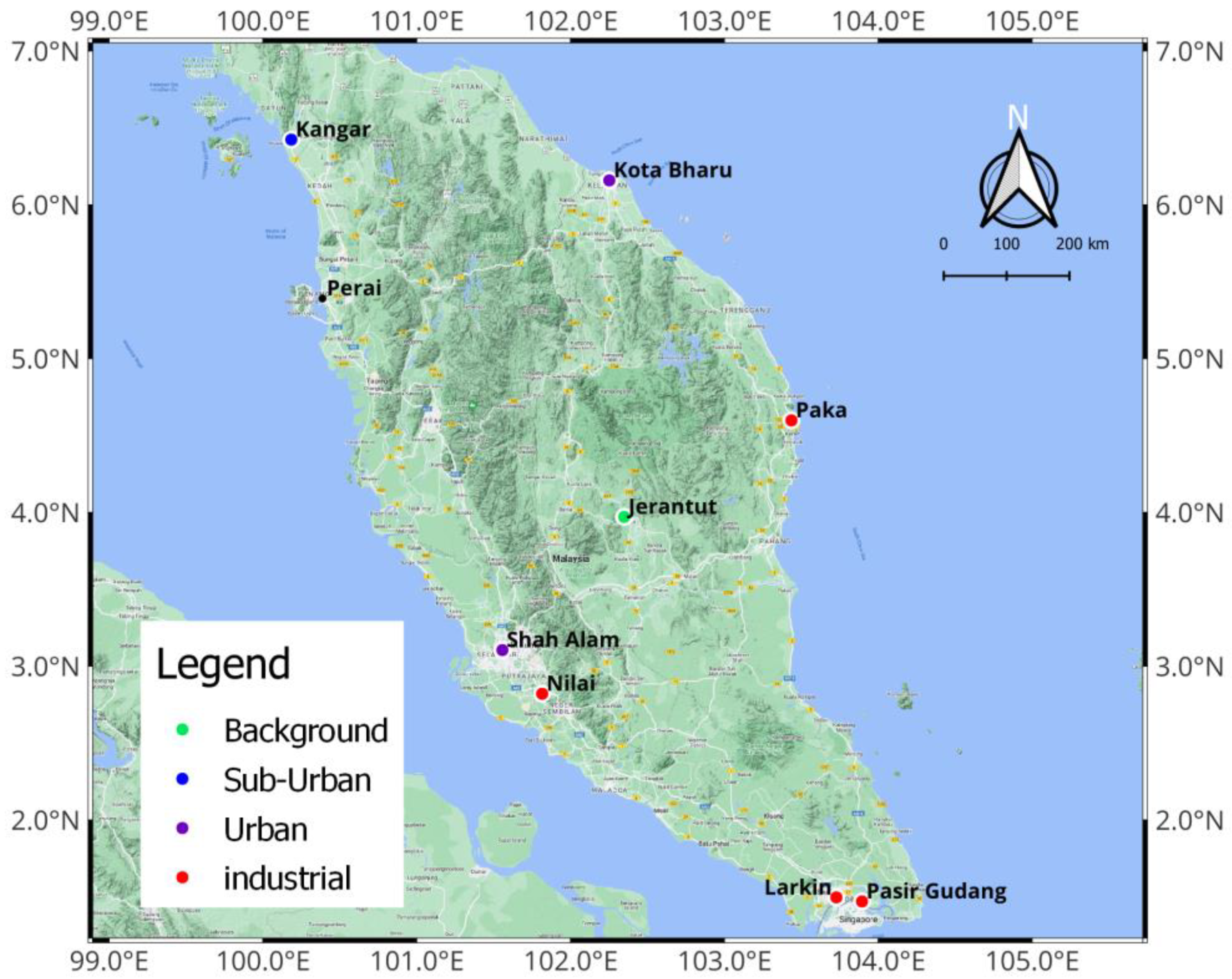
Nine monitoring stations were selected to represent Peninsular Malaysia. The research area covered the northern region (two monitoring stations), central region (two monitoring stations), southern region (two monitoring stations), eastern region (two monitoring stations) and background station (one station). The stations were Kangar, Perai, Shah Alam, Nilai, Larkin, Pasir Gudang, Paka, Kota Bharu and Jerantut, as illustrated in Figure 1. The coordinates and the details of the stations are summarized in Table 1.

Figure 1. Location of the nine monitoring stations.

Table 1. Detail description of the nine selected monitoring stations.

Station	State	Location	Coordinate	Region	Classification
Kangar	Perlis	Institut Latihan Perindustrian (ILP)	6°25.424′ N 100°11.046′ E	North	Sub-urban
Perai	Pulau Pinang	Sek. Keb. Cenderawasih, Taman Inderawasih	5°23.470′ N 100°23.213′ E		Industrial
Shah Alam	Selangor	Sek. Keb. Taman Tun Dr. Ismail Jaya	3°06.287′ N 101°33.368′ E	Centre	Urban
Nilai	Negeri Sembilan	Taman Semarak (Phase II)	2°49.246′ N 101°48.877′ E		Industrial
Larkin	Johor	Teacher Education Temenggong Ibrahim Campus	1°29.815′ N 103°43.617′ E	South	Industrial
Pasir Gudang	Johor	Sek. Men. Keb. Pasir Gudang 2	1°28.225′ N 103°53.637′ E		Industrial
Paka	Terengganu	Tenaga Nasional Berhad Quarters, Paka-Kertih	4°35.880′ N 103°26.096′ E	East	Industrial
Kota Bharu	Kelantan	Sek. Men. Keb. Tanjung Chat	6°09.520′ N 102°15.059′ E		Urban
Jerantut	Pahang	Meteorology Monitoring Station Batu Embun	3°58.238′ N 102°20.863′ E	-	Background

Kangar monitoring station is situated three kilometres away from a rice mill and a timber industry [54]. Mining quarries and landfills are the biggest potential sources of air pollution in Perlis. Perai is an administrative town that is situated on the south bank of the Perai River [55]. With a total area of 738 km², Perai is one of Peninsular Malaysia’s most densely populated districts. The Perai monitoring station is situated near heavily industrialised areas, where local industrial emissions and major road traffic emissions account for the majority of air pollution emissions [55].

With a large number of residential areas, educational facilities, commercial and industrial locations, Shah Alam is one of Malaysia’s most rapidly developing regions [56]. Shah Alam has a 290.3 km² area with a population of 700,000 [57]. According to Dominick et al. [27], there is a serious air quality problem in Shah Alam’s metropolitan area because of dust fallout and particulate matter on the jam-packed roadways, both of which are caused by vehicle emissions. Nilai is a quickly growing town that is surrounded by heavy traffic, periodic high particulate occurrences and industrial combustions, and it is located in a heavily industrialised part of the Malaysian central peninsular [28,58]. Larkin is a highly developed, densely populated industrial district that is encircled by important roadways, tourism destinations and other industrial areas [59]. The Tampoi and Larkin Industrial Park is within two kilometres of the Larkin monitoring station. A rising metropolis surrounded by residential and business areas, Larkin Sentral is not far from the Larkin monitoring station. The Pasir Gudang monitoring station is encircled by residential and business sectors within a two-to-three-kilometre range. The main industries are logistics and transportation, petrochemicals, fertiliser and cement manufacture, storage and distribution of palm oil, electroplating and a Tenaga Nasional Berhad power plant [57,59].

The Terengganu state town of Paka is located on the seaside. The monitoring station of Paka is located in a growing oil and gas region that is one-to-two kilometres from the important roads Kemaman-Dungun and Jerangau-Jabor Penghantar. Paka is an industrial zone including the PETRONAS Petrochemical Integrated Complex (PPIC), which connects the entire oil and gas value chain surrounding Paka [60]. Kota Bharu is the capital and largest city in the state of Kelantan with a total area of over 403 km². In Kota Bharu, the agricultural and industrial park Pengkalan Chepa is the main use of land. Vehicle emissions from nearby major roads have the biggest effects on the Kota Bharu monitoring station during morning and late afternoon rush hours [61,62]. Jerantut, the background station, is located in the center of Peninsular Malaysia. Natural woodland, agricultural terrain and Malaysian settlements surround the Jerantut station [63,64].

2.2. The Air Quality Monitoring Data

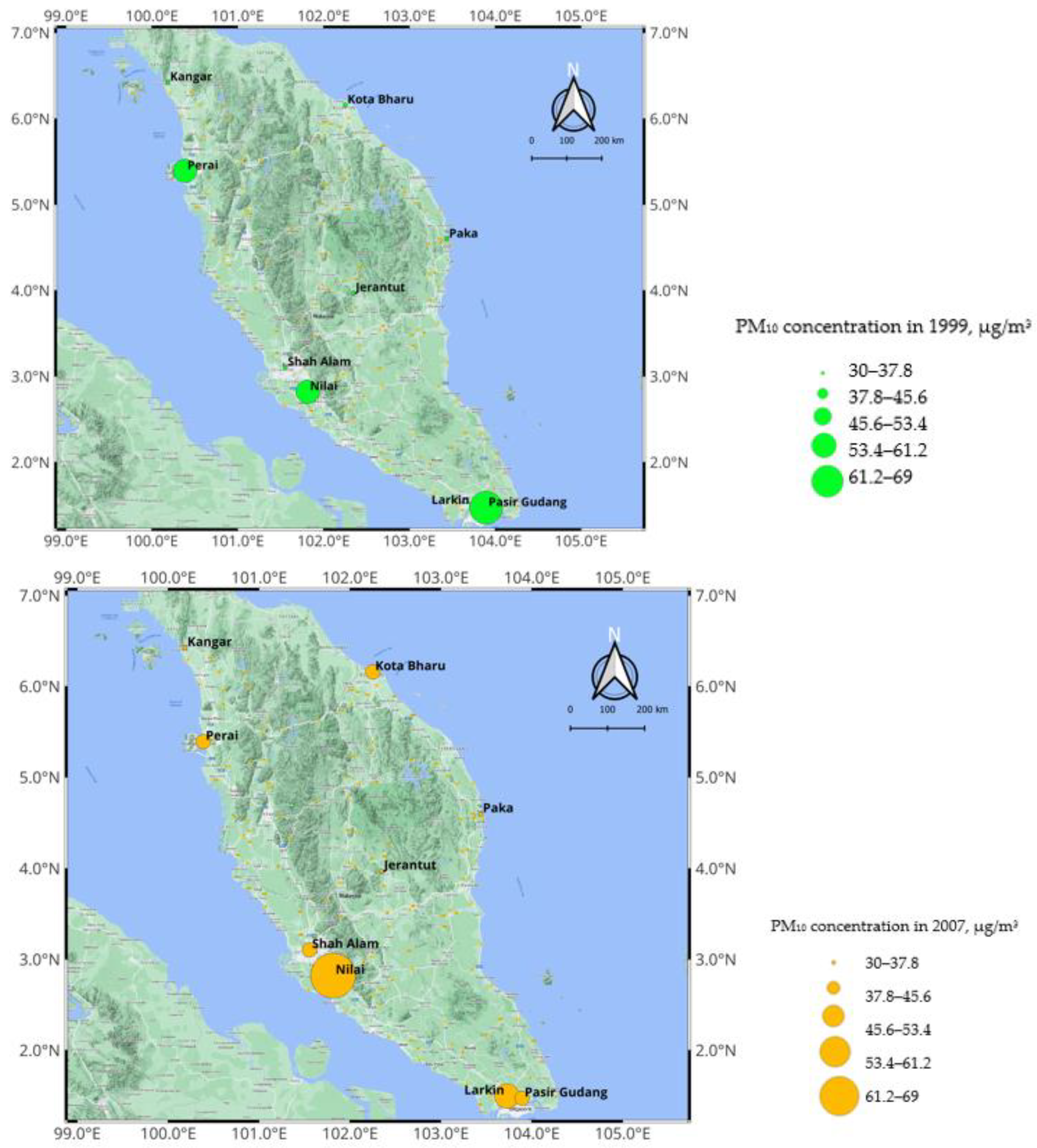
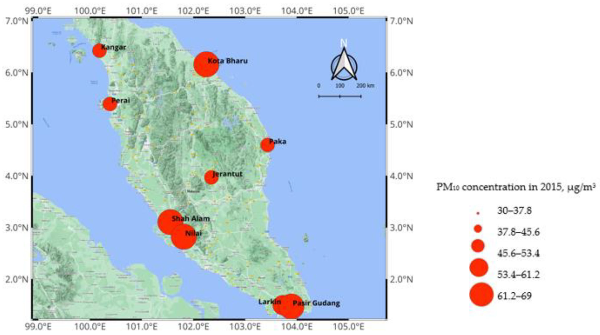
The Malaysian Department of Environment provided the data for the period of 1999 to 2015. The parameters used are the daily average of the particulate matter with an aerodynamic diameter less than 10 microns (PM₁₀; µg/m³) as a dependent parameter, while the independent parameters are nitrogen dioxide (NO_2; ppm), sulphur dioxide (SO₂; ppm), carbon monoxide (CO; ppm), ground-level ozone (O_3; ppm), temperature (T; °C), relative humidity (RH; %) and wind speed (WS; km/h). Table 2 summarises the dataset, and Figure 2 depicts the regional distribution of PM₁₀ concentrations for nine monitoring stations in 1999, 2007 and 2015.

Table 2. Air quality monitoring data.

Parameter	Symbol	Unit
Particulate matter	PM10	µg/m3
Nitrogen dioxide	NO2	ppm
Sulphur dioxide	SO2	ppm
Carbon monoxide	CO	ppm
Ground-level ozone	O3	ppm
Temperature	T; Temp	°C
Relative humidity	RH	%
Wind speed	WS	km/h

Figure 2. Spatial distribution of PM₁₀ concentrations in 1999, 2007 and 2015.

2.3. The Bayesian Model

Bayesian judgments are based on the Bayes theorem, a simple conclusion of conditional probability. The likelihood function, along with the parameter’s prior distribution, are multiplied to obtain the posterior distribution [65]. To calculate the parameter’s probability θ, the data D, the posterior distribution $Pr\left(\theta |D\right)$. The Bayes theorem is applied in the Bayesian statistics by using [53]

$$Pr(\left.\theta \right|D)=Pr(\left.D\right|\theta )\hspace{1em}\times \hspace{1em}\frac{Pr(\theta )}{Pr(D)}$$

(1)

where the evidence is

$$Pr(D)={\displaystyle \int d} \hspace{0.17em}\theta \hspace{0.17em}Pr(D\left|\theta )\right.\hspace{0.17em}Pr(\theta )$$

(2)

Posterior distribution, $Pr\left(\theta |D\right),$ is the belief in that parameter when data D is taken into account. The probability, $Pr\left(D|\theta \right),$ is the likelihood that the parameter θ may produce the data D. The prior, $Pr\left(\theta \right),$ is the initial probability of parameter θ without the data D [53,66]. The Bayesian theorem is as follows:

$$Pr (\mathrm{Posterior} \mathrm{distribution})\propto Pr \left(\mathrm{Likelihood}\right)\times Pr \left(\mathrm{Prior\; distribution}\right)$$

(3)

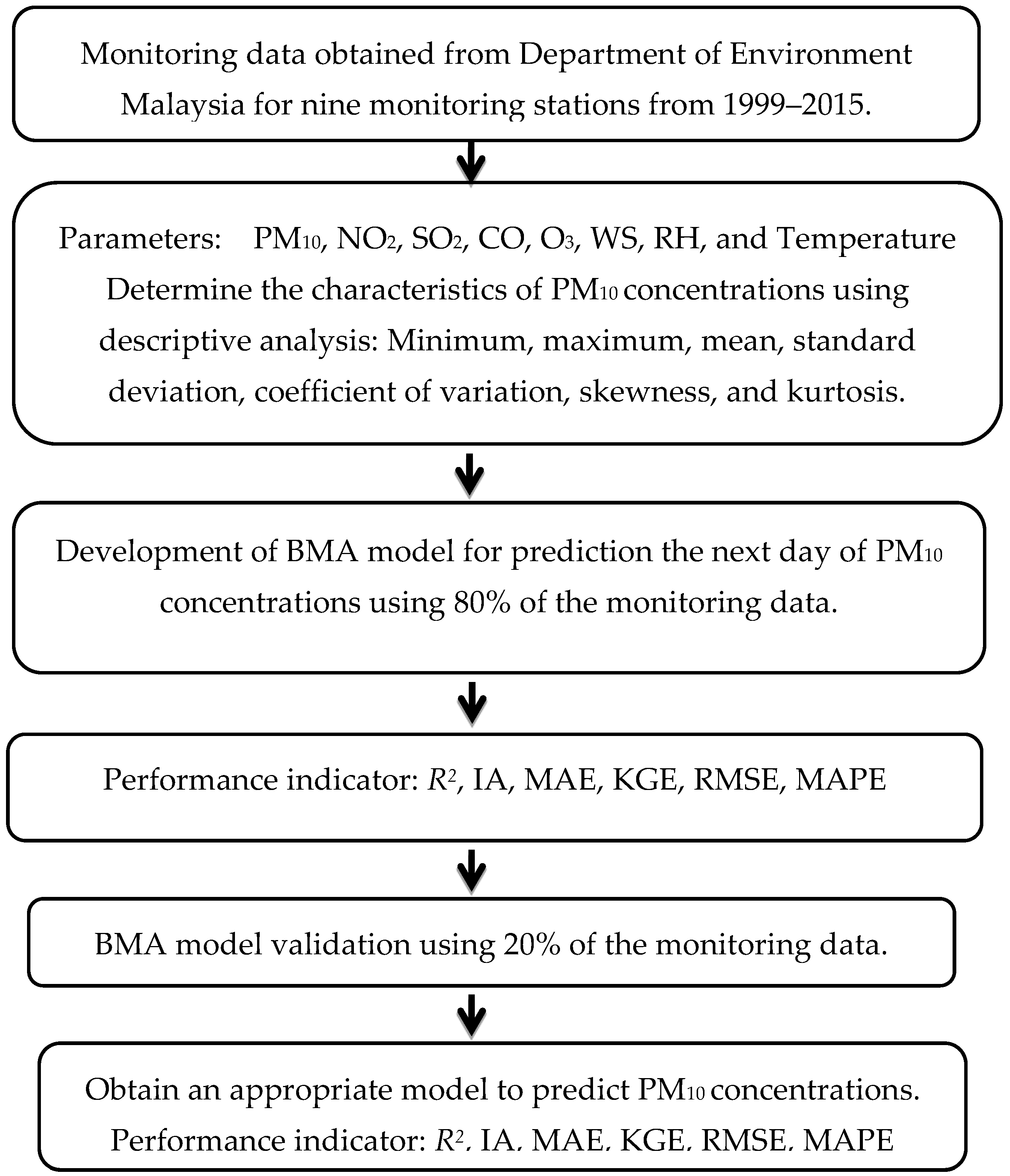
The Bayesian model averaging (BMA) technique is utilised so that PM₁₀ concentrations can be predicted. When making an inference, the BMA takes the parameter values from a large number of candidate models and uses the posterior distribution to calculate an average value for each model [67]. The concentrations of PM_10,D0, SO₂, NO₂, O₃, CO, temperature (T), wind speed (WS) and relative humidity (RH) are the model’s input variables. These data are provided to the model by the user. The first 80% of the monitoring data were utilised as training data in order to estimate the values of the model parameters, while the remaining 20% of the data were utilised for validation. Figure 3 depicts the research flowchart.

Figure 3. Research flowchart.

Priors can either be conjugate or informative depending on their function. When both the posterior distribution and the prior distribution have the same shape, a conjugate prior can be said to exist. Gamma and normal prior and likelihood distributions are employed for the analysis. The probability distribution function formula [57,68] is shown in Table 3, and the conjugate prior distributions that were employed and the resulting posterior distributions [68] are shown in Table 4.

Table 3. Probability distribution function formulas.

Distributions		Formula
Normal	pdf	$\begin{array}{l}f(x;\mu ,\sigma )=\frac{1}{\sigma \sqrt{2\pi }}\exp \left\{-\frac{1}{2}{\left(\frac{x-\mu }{\sigma }\right)}^2\right\}\\ for\hspace{0.33em}\sigma >0,\hspace{0.33em}x>-\infty \hspace{0.33em}and\hspace{0.33em}-\infty <\mu <\infty \end{array}$
	cdf	$\begin{array}{l}F(x;\mu ,\sigma )=\frac{1}{\sigma \sqrt{2\pi }}{\displaystyle \underset{-\infty }{\overset{x}{\int }}\exp }\left\{-\frac{1}{2}{\left(\frac{t-\mu }{\sigma }\right)}^2\right\}dt\\ for\hspace{0.33em}\sigma <0,\hspace{0.33em}x>-\infty \hspace{0.33em}and\hspace{0.33em}-\infty <\mu <\infty \end{array}$
Uniform	pdf	$f(x)=\left\{\begin{array}{l}\frac{1}{b-a}\\ 0\end{array}\right.\hspace{1em}\hspace{1em}a\le x\le b$
	cdf	$F(x)=\left\{\begin{array}{l}0\\ \frac{x-a}{b-a}\\ 1\end{array}\right.$$\begin{array}{l}\hspace{1em}\hspace{1em}x<0\\ \hspace{1em}\hspace{1em}a\le x\le b\\ \hspace{1em}\hspace{1em}x\ge b\end{array}$
Gamma	pdf	$f(x;\lambda ,\sigma )=\frac{1}{\sigma \Gamma (\lambda )}{\left(\frac{x}{\sigma }\right)}^{\lambda -1}\exp \left(-\frac{x}{\sigma }\right)$
	cdf	$\begin{array}{l}F(x;\lambda ,\sigma )=\frac{1}{\sigma \Gamma (\lambda )}{\left(\frac{x}{\sigma }\right)}^{\lambda -1}\exp \left(-\frac{x}{\sigma }\right)\\ for\hspace{0.33em}\sigma \ge 0\hspace{0.33em}\hspace{0.33em}and\hspace{0.33em}\hspace{0.33em}\sigma ,\lambda >0\end{array}$

$\mu$ is the location parameter; $\sigma$ is the scale parameter; $\lambda$ is the shape parameter; $\mathsf{\Gamma }$ is the gamma distribution.

Table 4. Prior distribution combined.

Conjugate Prior Distribution	Likelihood	Posterior Distribution
$N\left(\mu |{\mu }_0,\sum o\right)$	$N(\left.x\right|\mu ,\sum )$	$N\left(\mu {({\sum }_0^{-1}+n{\sum }^{-1})}^{-1}{({\sum }_0^{-1}{\mu }_0+n{\sum }^{-1}\overline{x})}^{-1},{({\sum }_0^{-1}+n{\sum }^{-1})}^{-1}\right)$
$Gamma\left.({\sigma }^{-2}\right|a,b)$	$N\left(x|\mu , {\sigma }^2\right)$	$Gamma\left({\sigma }^{-2}\right|a+n/2,b)+{\sum }_{i=1}^n{(x_i-\mu )}^2/2$

n is the number of monitoring data; $\overline{x}$ is the mean of $x$; ${\sigma }^2$ is the variance.

The posterior distributions of the top models are averaged to complete the BMA, which is the uncertainty model. The primary idea behind the BMA is to compare all potential models in order to choose the best one [69]. Leamer [67] suggested using the BMA to implement the linear regression model. Assume a regression model with a constant term, ${\beta }_0$, and the potential independent parameters, which are PM_10,D0, T, RH, WS, NO₂, SO₂, CO and O₃:

$${\mathrm{PM}}_{10,\mathrm{D}1}={\beta }_0+{\beta }_1{\mathrm{PM}}_{10,\mathrm{D}0}+{\beta }_2\mathrm{T}+{\beta }_3\mathrm{RH}+{\beta }_4\mathrm{WS}+{\beta }_5{\mathrm{NO}}_2+{\beta }_6{\mathrm{SO}}_2+{\beta }_7\mathrm{CO}+{\beta }_8{\mathrm{O}}_3+\epsilon$$

(4)

A weighted average of all models is calculated by BMA for all conceivable combinations of independent parameters. If independent parameters contain K potential parameter, this means estimating $2^k$ parameter combinations, and thus $2^k$ models. Given the number of regressors, $2^k$ different combinations of right-hand side parameters are indexed by $M_j$ for $j=1, 2, 3,\dots ,2^k$. The posterior distribution of any relevant coefficient, ${\beta }_h$, given the data D, is the following:

$$Pr({\beta }_h|D)={\displaystyle \sum _{j:{\beta }_{hy}\in M_j}^{}Pr({\beta }_h}|M_j,D)Pr(M_j|D)$$

(5)

The BMA uses each model’s posterior probability, $Pr\left(M_j|D\right),$ as weights. The posterior probability of $M_j$ is equal to the ratio of its likelihood to the sum of all likelihoods in the model [70]. This is the average posterior distribution under each model, weighted by the posterior probabilities of each model.

$$Pr(M_j|D)=Pr(D|M_j)\frac{Pr(M_j)}{Pr(D)}=Pr(D|M_j)\frac{Pr(M_j)}{{\displaystyle \sum _{i=1}^{2^k}Pr(D|M_i)}Pr(M_i)}$$

(6)

where,

$$Pr(D|M_j)={\displaystyle \int Pr(D|{\beta }^j,M_j)}\hspace{0.33em}Pr(\left.{\beta }^j\right|M_j)d{\beta }^j$$

(7)

and ${\beta }^j$ is the vector of parameters from model $M_j, Pr\left(B^j|M_j\right),$a prior probability distribution assigned to the parameters of model $M_j$, and $Pr\left(M_j\right)$ is the prior probability that $M_{j }$is the true model [39,48]. The estimated posterior means and standard deviations of $\widehat{\beta }=({\widehat{\beta }}_0,{\widehat{\beta }}_1,\dots ,{\widehat{\beta }}_k)$ are then constructed.

$$E\left[\widehat{\beta }|D\right]={\displaystyle \sum _{j=1}^{2^k}\widehat{\beta }Pr(M_i|D)},$$

(8)

$$V\left[\widehat{\beta }|D\right]={\displaystyle \sum _{j=1}^{2^k}\left(Var\left[\beta \left|D,M_j\right.\right]+{\widehat{\beta }}^2\right)Pr(M_j|D)}-E{\left[\beta |D\right]}^2$$

(9)

where,

$${\widehat{\beta }}_k=E\left[\widehat{\beta }\left|D,M_k\right.\right]$$

(10)

The BMA software performs BMA analysis using a simple BIC (Bayesian Information Criterion) to create the prior probability of regression coefficients [39,71]. Then, a specific BIC difference according to Table 5 is used to compare and identify models $M_j$, to $M_i$, which are more likely to be included in the final set of good models [39,72]. The remaining models are attributed to Occam’s Window.

Table 5. Evidence levels that match to BIC difference values for $M_j$, against $M_i$.

BIC (Bayesian Information Criterion) Difference	Evidence
0–2	Weak
3–6	Positive
7–10	Strong
>10	Very strong

The model component of the BMA model is chosen using the Occam’s Window technique as given in Equation (11). The Occam’s Window technique, according to Madigan and Raftery [72], chooses the BMA model component depending on the posterior probability of the model. A model must satisfy the following equation in order to be accepted.

$$A^{\prime }=\left\{M_j:\frac{{\max }_i(\mathrm{Pr}(M_i\left|D))\right.}{\mathrm{Pr}(M_j\left|D)\right.}\le \hspace{0.33em}C\right\}$$

(11)

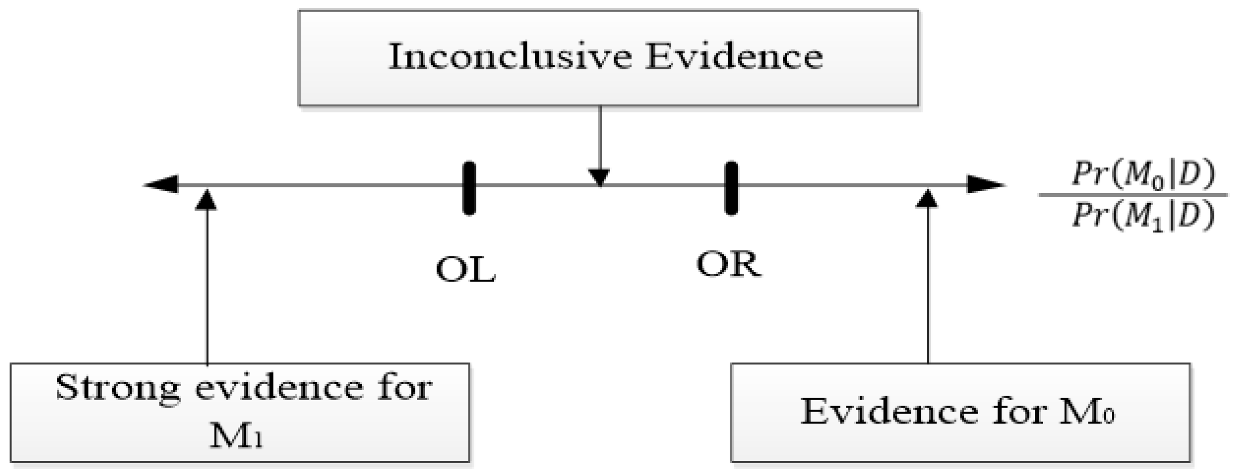
where $A^{\prime }$ is the posterior odds to the model j, and C values of 20 is equivalent to $\alpha =5\%$, using the test criteria with p-value [72]. A model is excluded from the BMA model and needs to be eliminated from the Equation (11) if its value is larger than 20. A model will be included in the BMA model in Equation (11) if its value is less than or equal to 20. The user can select a maximum ratio for excluding models in Occam’s Window (OR). The default value of the ratio is 20 [39,72]. Occam’s Window, which provides an interpretation of the posterior probability for the nested models, is shown in Figure 4. When comparing two models, the interpretation of the ratio of posterior model probabilities, $M_1$ and $M_0$ is as follows:

Figure 4. Interpreting the posterior chances for nested models using Occam’s Window. “Adapted from Madigan and Raftery [72].

1.

Consider $M_0$ instead of $M_1$ if the log posterior odd is positive (the data support the smaller model).

2.

If the log posterior odd is small and negative, which indicates that the evidence is weaker against the smaller model, then both models should be taken into consideration.

3.

Consider $M_1$ and reject $M_0$ if the log posterior odds are negative and large, (smaller than $O_L=-\log (C)$ where C is defined by Equation (11)) [48,72].

2.4. Performance Indicator

Calculating the performance indicators allows for an evaluation of the BMA model’s performance. Performance measures included the coefficient of determination (R²), index of agreement (IA), Kling-Gupta efficiency (KGE), normalised absolute error (NAE), root mean square error (RMSE) and mean absolute percentage error (MAPE). To choose a suitable BMA model for PM₁₀ concentration prediction, the acquired results were assessed. The performance indicator equation is shown in Table 6.

Table 6. Performance indicators [16,28,29].

Performance Indicator	Equation	Criteria
R2	$R^2={\left(\frac{1}{N}\frac{{\displaystyle \sum _{i=1}^N(P_i}-\overline{P})(O_i-\overline{O})}{S_{pred}.S_{obs}}\right)}^2$	Range between [0, 1] with the best value of 1.
IA	$IA=1-\left(\frac{{\displaystyle \sum _{i=1}^N(P_i}-O_i{)}^2}{{\displaystyle \sum _{i=1}^N\left|P_i-\overline{O}\right|+{\left|O_i-\overline{O}\right|}^2}}\right)$
KGE	$KGE=\sqrt{{\left(\gamma \prime - 1\right)}^2+{\left(\alpha - 1\right)}^2+{\left(\mathrm{r} - 1\right)}^2}$
MAE	$MAE=\frac{1}{N}{\displaystyle \sum _{i=1}^N\left|P_i\right.}-\left.O_i\right|$	The best model has the values closer to zero (0) or the smallest values.
RMSE	$RMSE=\sqrt{\frac{1}{N}{\displaystyle \sum _{i=1}^N\left(P_i\right.}-{\left.O_i\right)}^2}$
MAPE	$MAPE=\frac{{\displaystyle \sum _{i=1}^N\left|\frac{O_i-P_i}{O_i}\right|}}{N}\times 100$

$N$ is number of observations data; $O_i$ is the observed data; $\overline{O}$ is the mean of observed data; $P_i$ is the predicted data; $\overline{P}$ is the mean of predicted data; $S_{obs}$ is the standard deviation of observed data, $S_{pred}$ is the standard deviation of predicted data, γ′ is error in bias, α is the error in flow variability, and r is correlation.

3. Results and Discussion

3.1. Descriptive Statistics of PM₁₀ Level

The descriptive statistics were applied to the daily average of PM₁₀ concentrations data and the values are useful in determination of pollution status and characteristics of PM₁₀ concentrations at each monitoring station from 1999 to 2015. The data summary of PM₁₀ concentrations at all study areas is shown in Table 7. Overall, Jerantut, the background station, recorded the lowest mean value (38.4 μg/m³) compared to other areas. The PM₁₀ level in the east Peninsular Malaysia region (Paka and Kota Bharu) was observed to be less compared to the concentration in the centre (Shah Alam and Nilai) and north region (Kangar and Perai) of Peninsular Malaysia. The west coast region is more developed and urbanized compared to the east coast of Peninsular Malaysia, and it is separated by Banjaran Titiwangsa—a range of mountain where the Jerantut (the background station) is located. In addition, a higher variation of PM₁₀ level can be observed in the industrial areas (Perai, Shah Alam and Nilai) with the standard deviation ranging from 23.39 to 26.89, compared to other stations that recorded <20. All stations show a highly skewed distribution of PM₁₀ concentration, with the value of skewness >1.

Table 7. The descriptive statistics of daily average of PM₁₀ concentrations (μg/m³) from 1999 to 2015.

Station	Kangar	Perai	Shah Alam	Nilai	Larkin	Pasir Gudang	Paka	Kota Bharu	Jerantut
Number of data set	6209	6209	6209	6178	6209	6179	6209	6209	6209
Minimum	4	13	14	15	13	15	14	12	11
Maximum	363	317	587	327	349	461	238	189	271
Mean	40.74	53.77	53.61	59.19	43.17	51.21	37.34	42.06	38.35
Std. Deviation	16.50	24.80	26.89	23.39	18.54	19.54	13.81	15.63	15.99
Coefficient of variation	0.41	0.46	0.50	0.40	0.43	0.38	0.37	0.37	0.42
Skewness	3.09	1.67	4.64	3.15	4.05	4.65	4.30	1.82	3.19
Kurtosis	36.77	5.55	53.38	20.82	37.01	57.04	37.88	6.97	24.01

The annual average of PM₁₀ concentrations at nine monitoring stations from 1999–2015 is summarized in Table 8. The analysis provides a summary of the status of air quality in Peninsular Malaysia. The annual average of PM₁₀ concentrations for nine monitoring stations is compared to the Malaysian Ambient Air Quality Standard Interim Target 1 (2015), where the allowable limit for PM₁₀ concentrations is 50 µg/m³ per year. From the results, Shah Alam, Nilai, Larkin, Pasir Gudang, Paka and Kota Bharu exceeded the Interim Target limit in 2015. The unhealthy air quality is recorded in those areas due to the high level of PM₁₀ concentrations by the transboundary pollution and open-burning activities within the country, especially during the prolonged hot and dry periods. In the years 2005, 2006 and 2015 almost the entire country was affected by transboundary pollution resulting from forest and land fires in Sumatra, Indonesia [73,74,75]. The sources of air pollution over Malaysia are mostly motor vehicle emissions, industries, biofuel burning [76], heat and power plants and open combustion [13], thus favouring the accumulation of PM₁₀ concentrations around the urban and industrialized areas [77].

Table 8. The annual average of PM₁₀ concentrations for all locations from 1999–2015, Units = µg/m³.

Year	Kangar	Perai	Shah Alam	Nilai	Larkin	Pasir Gudang	Paka	Kota Bharu	Jerantut
1999	33	52 *	35	45	34	55 *	38	34	37
2000	37	55 *	39	59 *	34	50 *	37	40	32
2001	38	57 *	43	54 *	33	49	36	37	35
2002	44	74 *	78 *	59 *	37	49	42	37	36
2003	43	79 *	58 *	55 *	38	48	38	40	36
2004	54 *	91 *	67 *	61 *	50 *	46	33	47	44
2005	59 *	78 *	64 *	63 *	36	46	32	43	50 *
2006	43	50 *	56 *	63 *	56 *	47	34	40	45
2007	38	45	45	62 *	55 *	43	32	40	38
2008	34	38	54 *	56 *	40	51 *	38	38	42
2009	35	39	53 *	56 *	44	57 *	38	43	36
2010	36	40	48	56 *	42	49	35	42	34
2011	38	46	54 *	59 *	44	45	38	46	36
2012	35	42	48	61 *	41	51 *	32	39	34
2013	39	39	47	58 *	44	51 *	35	42	34
2014	39	42	55 *	64 *	45	50 *	44	41	33
2015	47	47	66 *	70 *	60 *	65 *	53 *	67 *	49

* denotes exceed Malaysia Ambient Air Quality Standard IT-1 (2015) of 50 µg/m³ per year, Malaysia Ambient Air Quality Standard IT-2 (2018) of 45 µg/m³ per year, Malaysia Ambient Air Quality Standard (2020) of 40 µg/m³ per year.

Peninsular Malaysia had experienced deterioration of air quality from August to September 2015 during southwest monsoon due to forest fires and massive land burning in Indonesia. An unhealthy air quality status was recorded in 34 areas in the country, the first time in Malaysia’s history since 1997. The API reading reached 200, and due to unhealthy air quality status, all schools in Kuala Lumpur, Selangor, Putrajaya, Negeri Sembilan and Melaka were closed on 15 September 2015 [78]. There were a number of forest and peatland fires that slightly deteriorated the air quality status in the country, but they were not prolonged due to the humid weather all year round. The PM₁₀ concentrations remained as the predominant pollutant that had caused unhealthy conditions due to forest and peatland fires [73].

3.2. Bayesian Model Averaging (BMA)

Table 9 shows the BMA models for nine study areas. The BMA models have been established and, in turn, validated. Generally, it can be observed that the previous PM₁₀ concentration (PM_10,D0) was the most contributed parameter regarding the PM_10,D1 prediction model for all areas. Weather parameters such as relative humidity and wind speed were significant parameters in the centre (Shah Alam, Nilai), south (Larkin) and east (Paka) of the Peninsular Malaysia, including Jerantut. Significant parameters are a positive coefficient in the model, indicating that if the value of the independent parameter increases, the mean of the dependent parameters tends to increase as well. A negative coefficient indicates that the dependent parameters tend to decrease as the independent variable increases. However, temperature was only listed in the BMA models of Shah Alam and Pasir Gudang. Gases pollutants such as NO₂, O₃ and CO were noticed in the BMA models of Kangar, Perai, Larkin, Pasir Gudang and Kota Bharu, most of them being industrial areas.

Table 9. Bayesian model averaging (BMA) model for prediction of the next-day PM₁₀ (PM_10,D1).

Region	Station	BMA Model
North	Kangar	PM10,D1 = 10.283 + 163.616O3 + 0.759PM10,D0
	Perai	PM10,D1 = 12.272 − 9.879CO + 0.893PM10,D0
Centre	Shah Alam	PM10,D1 = 89.618 + 1.044WS − 0.987T − 0.682RH + 0.764PM10,D0
	Nilai	PM10,D1 = 46.79 − 0.664WS − 0.480RH + 0.705PM10,D0
South	Larkin	PM10,D1 = 15.450 − 0.392WS − 4.143CO + 0.775PM10,D0
	Pasir Gudang	PM10,D1 = 7.923 + 0.371T + 261.238NO2 + 0.639PM10,D0
East	Paka	PM10,D1 = 4.016 + 0.283WS + 0.045RH + 0.743PM10,D0
	Kota Bharu	PM10,D1 = 12.910 − 0.131RH + 698.4NO2 + 275O3 − 4.194CO + 0.731PM10,D0
Background station	Jerantut	PM10,D1 = 24.154 − 1.191WS − 0.148RH + 0.796PM10,D0

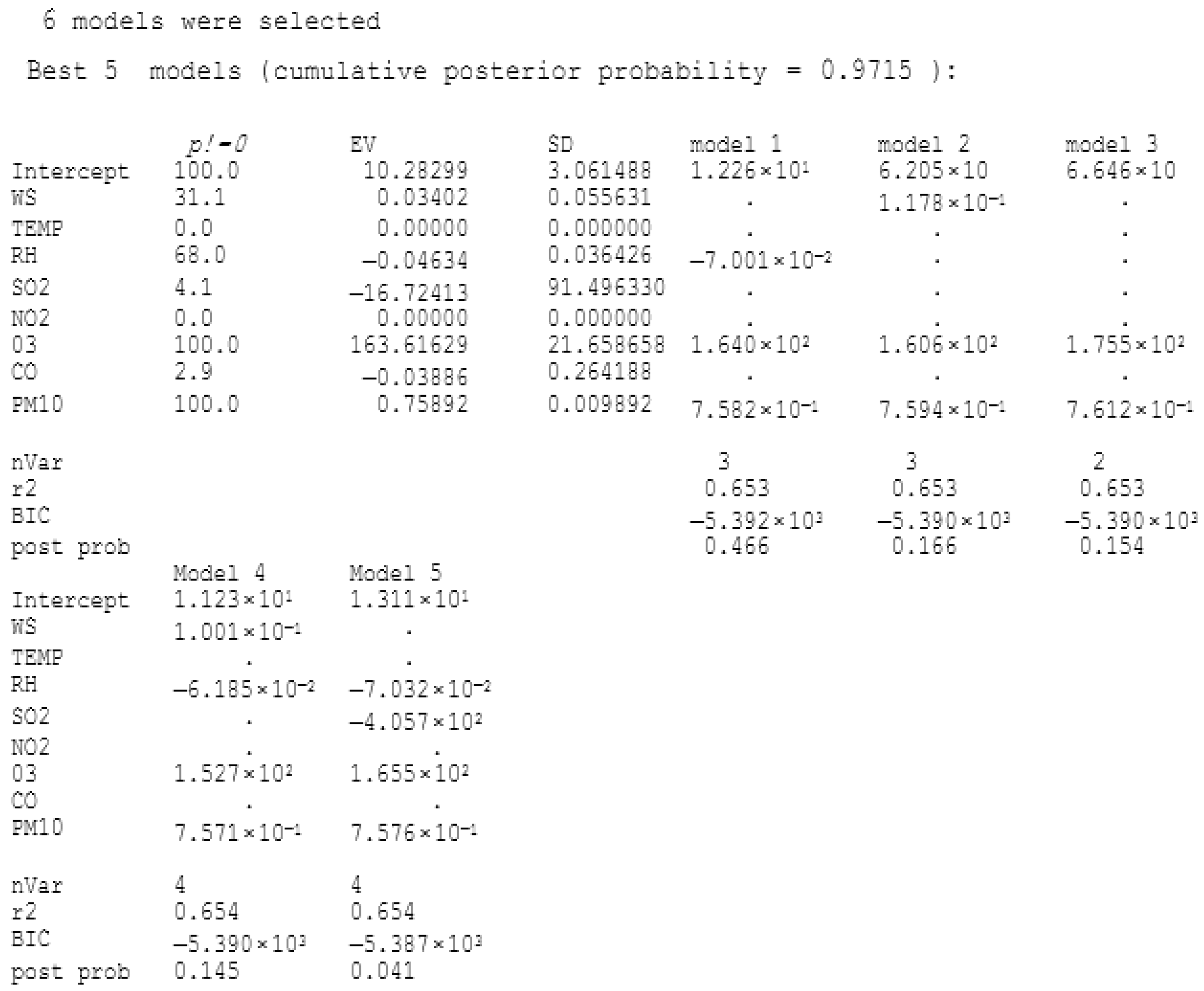
An overview of the BMA output for Kangar station is shown in Figure 3. The column labelled “p! = 0” in Figure 5 depicts the percentage of posterior probability that the parameter is included in the model. The “EV” column contains the BMA posterior mean. The posterior standard deviation for each parameter in the BMA is shown in the “SD” column. The parameter estimations for the five best models, when the parameters were present, are shown in the next five columns.

Figure 5. An overview of the BMA’s output for the Kangar.

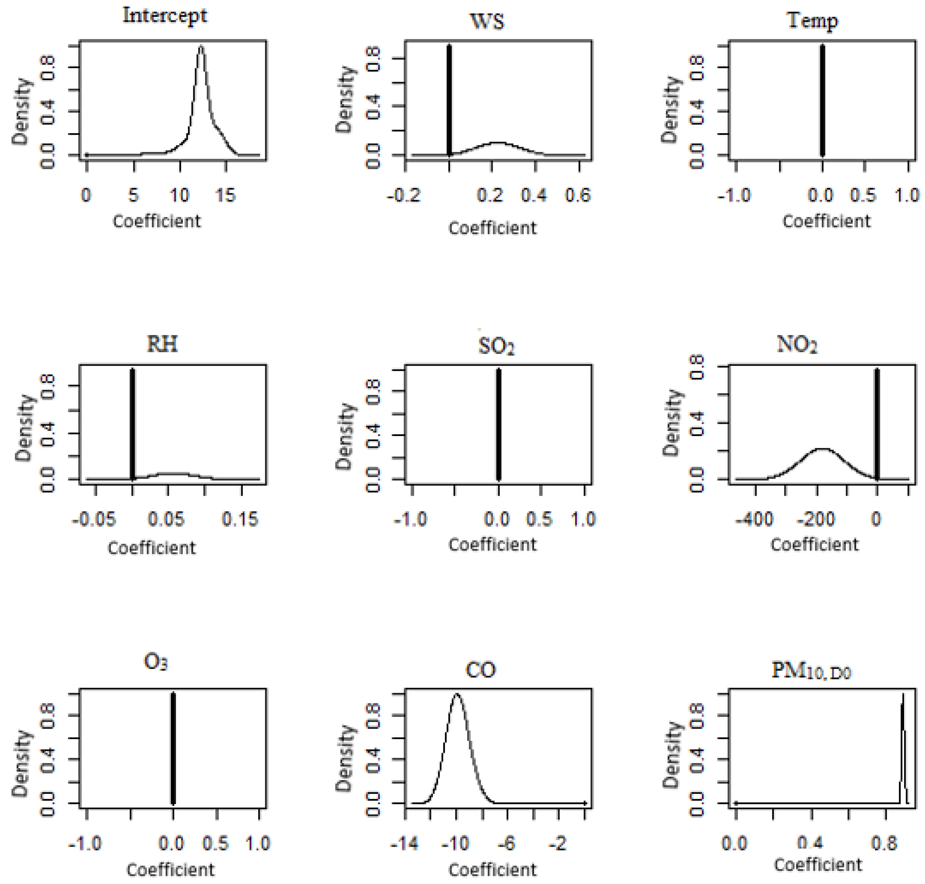
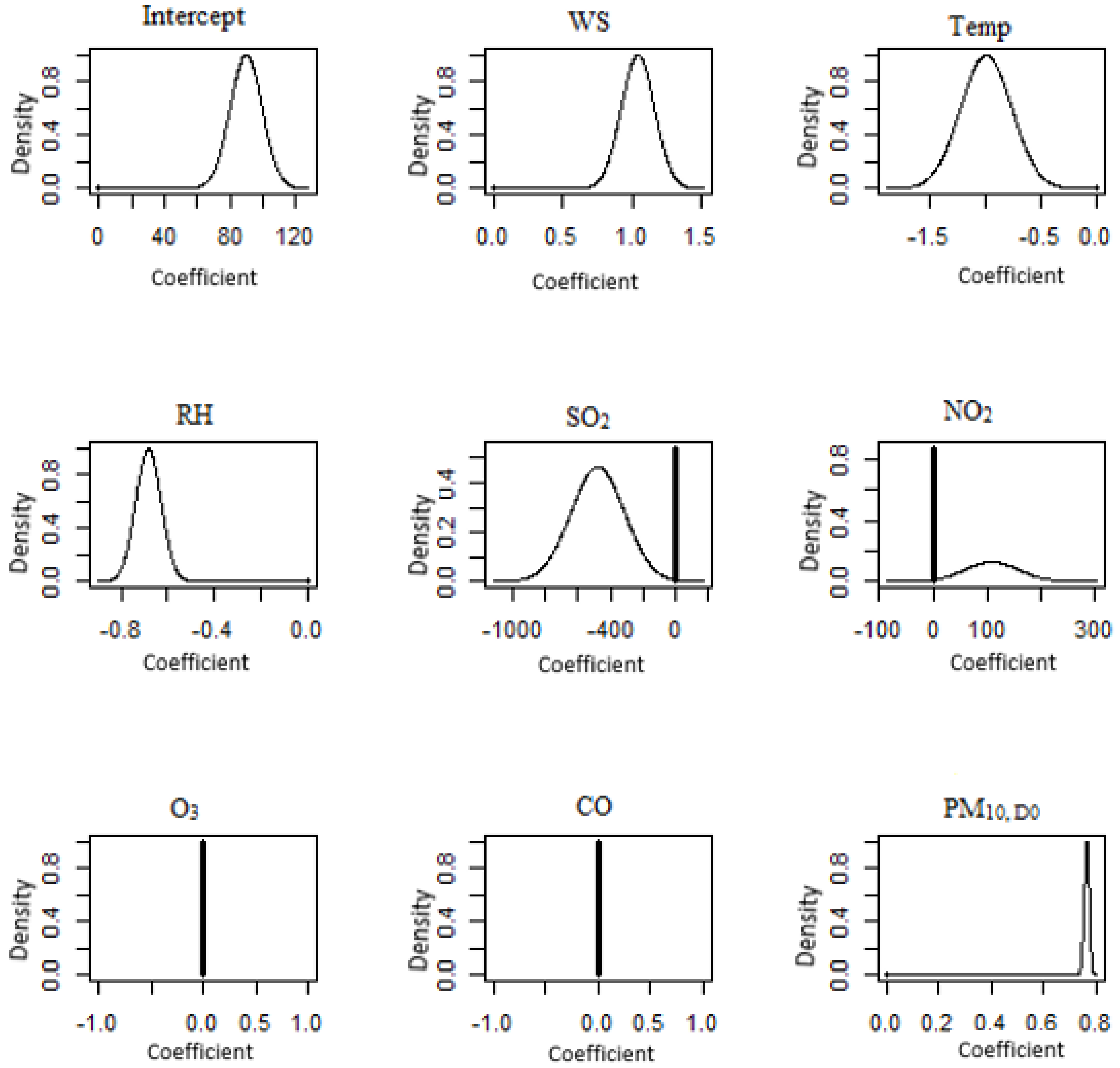
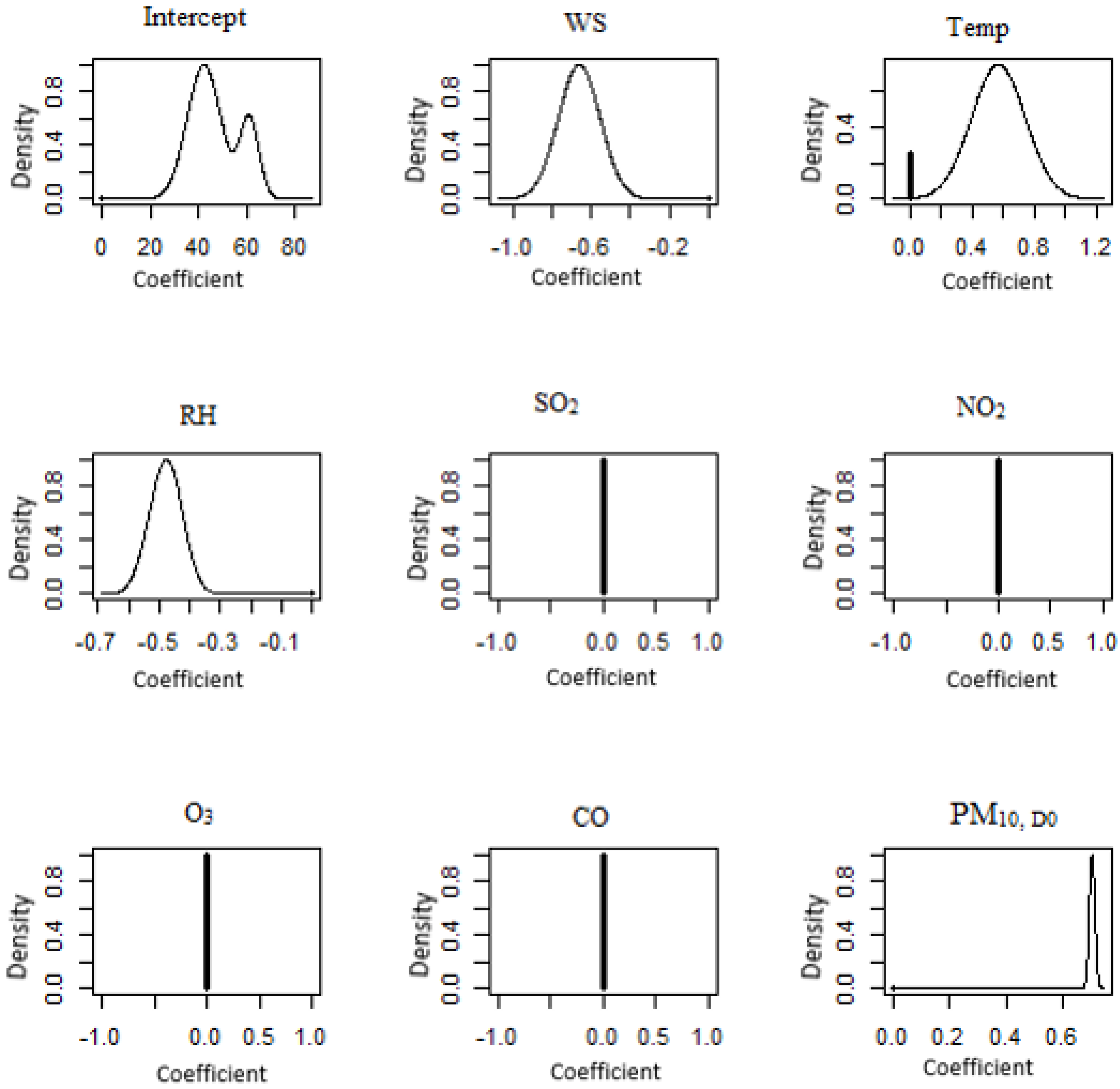
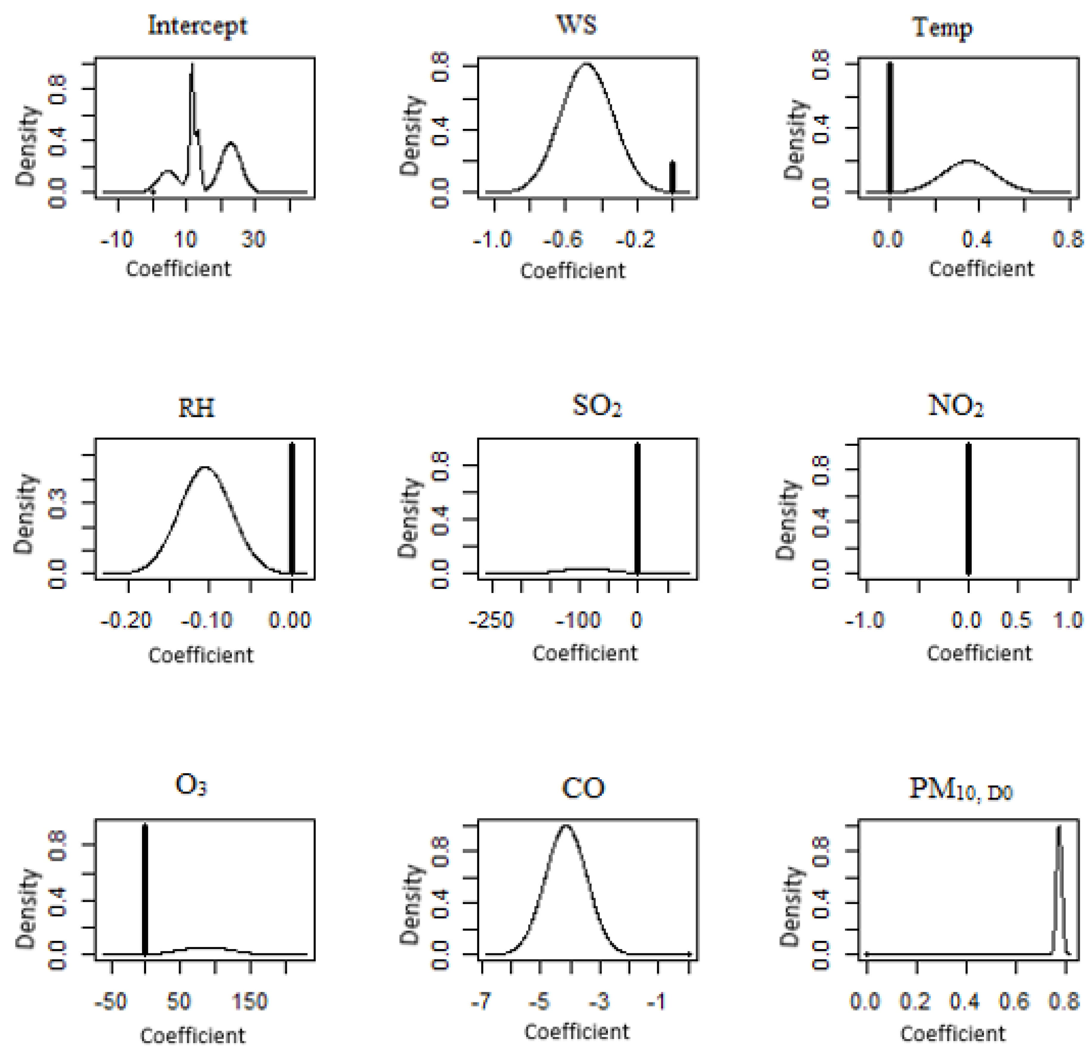
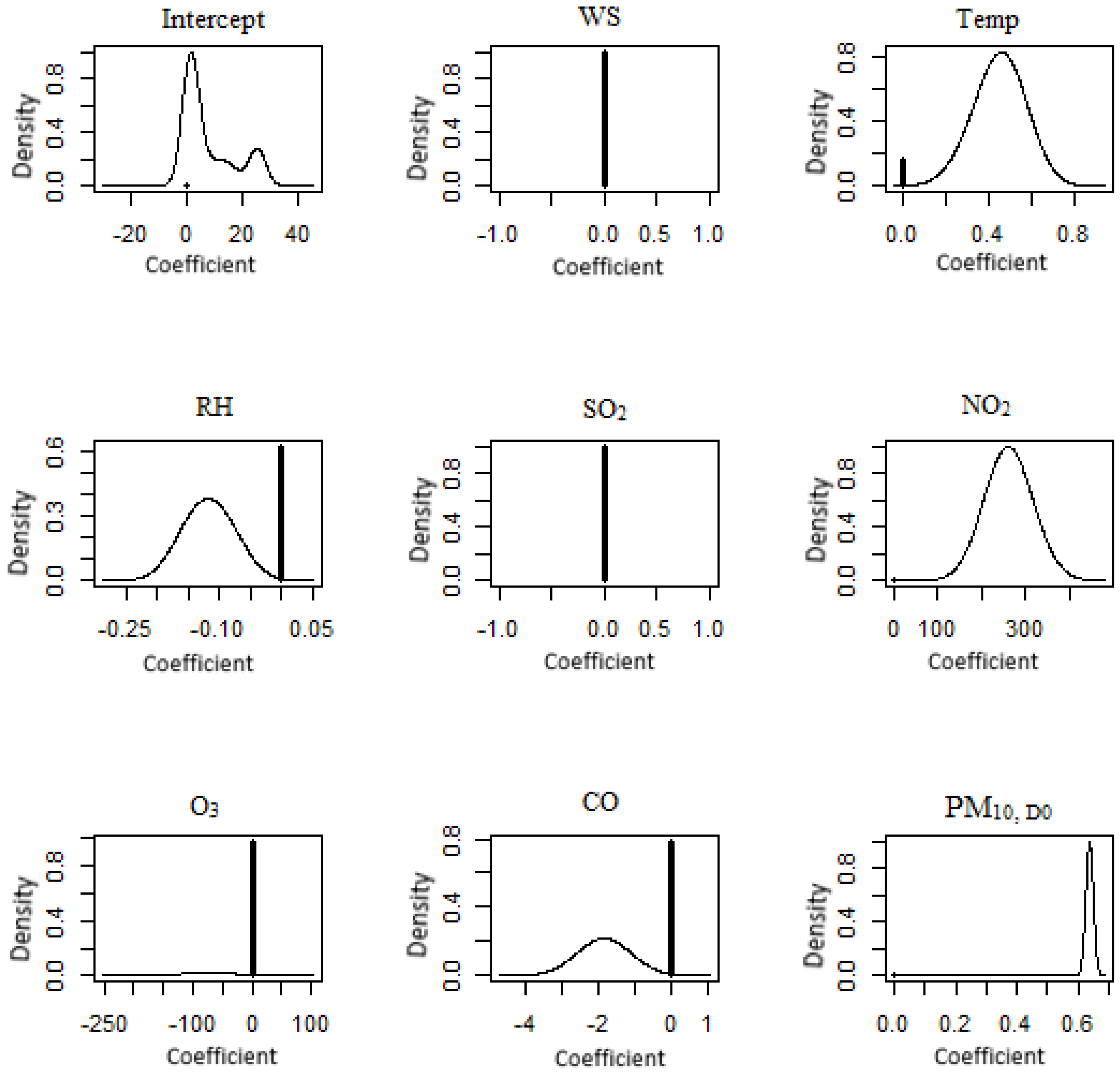
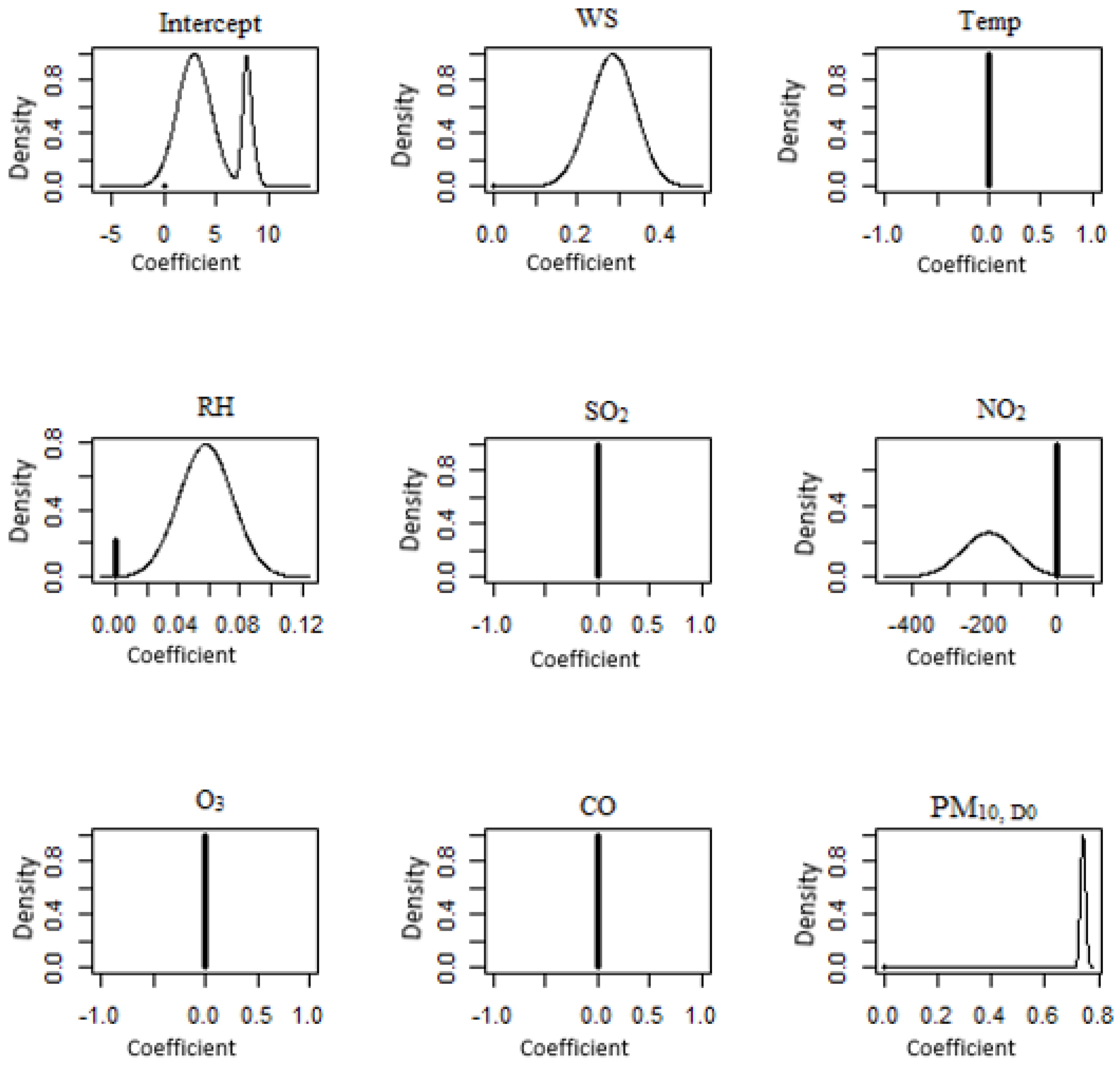
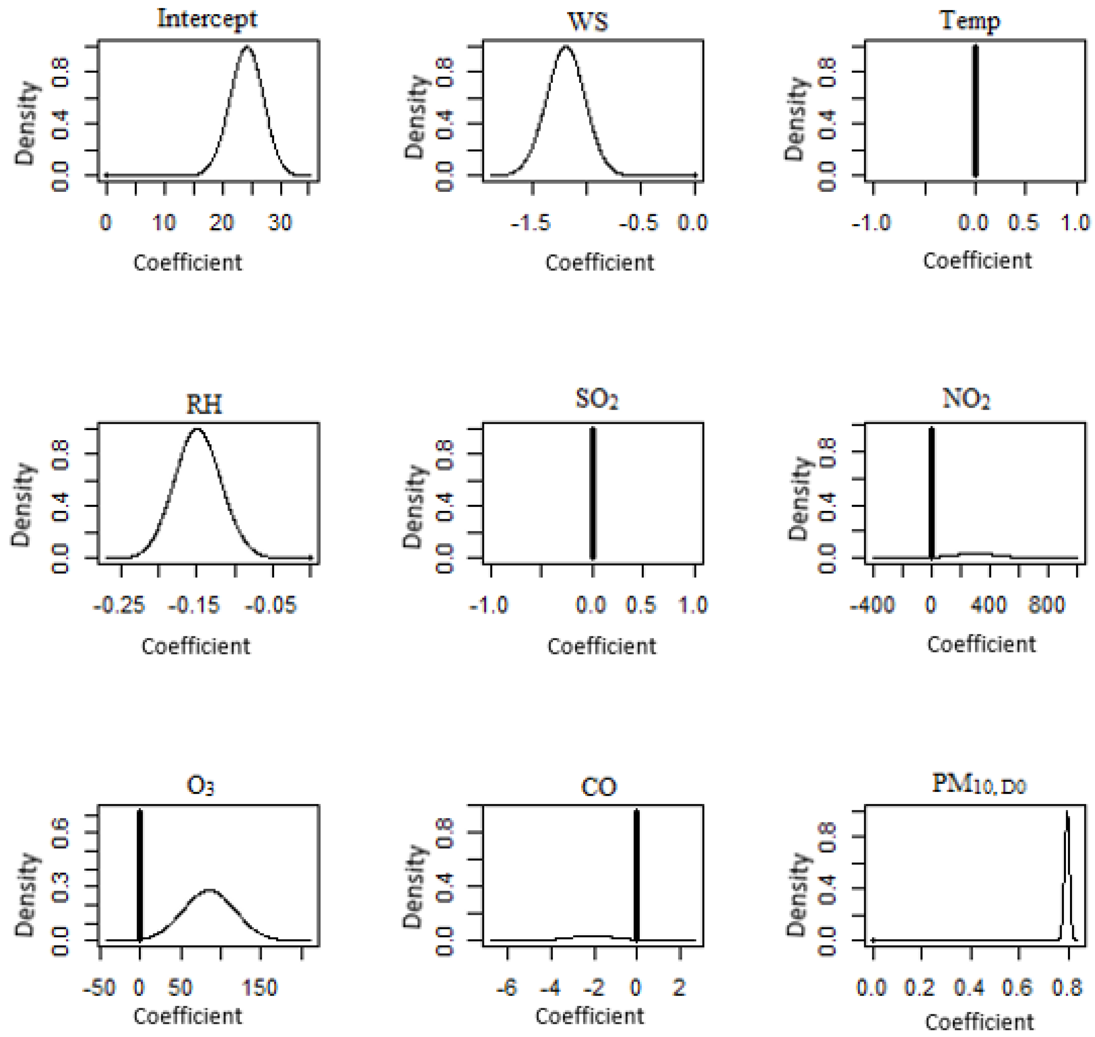
Figure 6, Figure 7, Figure 8, Figure 9, Figure 10, Figure 11, Figure 12, Figure 13 and Figure 14 provide an overview of the BMA posterior distribution for each monitoring station. The spike at zero indicates the possibility that the parameter is not included in the model. The peak at 0 represents the likelihood that the parameter does not exist in the model. Given that the parameter is included in the model, the curve displays its posterior density.

Figure 6. BMA posterior distributions for the northern region of Peninsular Malaysia (Kangar). Symbol ⁺ denotes the initial point of 0.

Figure 7. BMA posterior distributions for the northern region of Peninsular Malaysia (Perai). Symbol ⁺ denotes the initial point of 0.

Figure 8. BMA posterior distributions for the centre region of Peninsular Malaysia (Shah Alam). Symbol ⁺ denotes the initial point of 0.

Figure 9. BMA posterior distributions for the centre region of Peninsular Malaysia (Nilai). Symbol ⁺ denotes the initial point of 0.

Figure 10. BMA posterior distributions for the south region of Peninsular Malaysia (Larkin). Symbol ⁺ denotes the initial point of 0.

Figure 11. BMA posterior distributions for the south region of Peninsular Malaysia (Pasir Gudang). Symbol ⁺ denotes the initial point of 0.

Figure 12. BMA posterior distributions for the east region of Peninsular Malaysia (Paka). Symbol ⁺ denotes the initial point of 0.

Figure 13. BMA posterior distributions for the east region of Peninsular Malaysia (Kota Bharu). Symbol ⁺ denotes the initial point of 0.

Figure 14. BMA posterior distributions for the background station (Jerantut). Symbol ⁺ denotes the initial point of 0.

Wind speed, temperature, relative humidity, ozone, carbon monoxide and PM₁₀ make up the average of the elements that are included in the BMA posterior distribution for the next-day PM₁₀ level prediction. Rahman et al. [79] proved that PM₁₀ concentrations have a substantial association with both relative humidity and wind speed. It was determined that high wind speed has a substantial influence on lowering air pollutants, since it lessens the tendency of pollutants to accumulate and disperse in the air. This discovery was made possible by the fact that high wind speed creates more wind. In addition, Elbayoumi et al. [80] discovered that the temperature-related meteorological parameter has a substantial impact on the PM₁₀ concentration. Alterations in the temperature of the surrounding environment, on the other hand, have an impact on the weather’s predictability and, as a consequence, disrupt PM₁₀ concentrations.

The posterior BMA distributions for both the Kangar (Figure 6) and the Perai (Figure 7) show that the BMA posterior distribution of the coefficient of O₃ and PM₁₀ on that day is incorporated into the model, so that it can be applied to the Kangar monitoring station. After the harvesting season is through, open fires begin in the rice paddies over most of the district of Perlis. There is a possibility that the elevated PM₁₀ concentrations at the Kangar monitoring site were caused in part by the dispersion of particulate matter during days with strong winds [64]. The peak at 0 represents the chance that the model does not include the characteristics of wind speed, temperature, relative humidity, sulphur dioxide, nitrogen dioxide or carbon monoxide. The BMA posterior distribution of the coefficient of carbon monoxide and PM₁₀ for that day at the Perai monitoring station is included in the model. The spike at 0 shows that there is a possibility that the model does not contain the parameters for wind speed, temperature, relative humidity, sulphur dioxide, nitrogen oxide and oxygen.

The posterior BMA distributions for Shah Alam (Figure 8) and Nilai (Figure 9) included the parameters of wind speed, temperature, relative humidity and PM₁₀ concentration that made up the BMA posterior distribution of the coefficient in the model for the Shah Alam monitoring station. The likelihood is that the parameters that are missing from the model are sulphur dioxide, nitrogen dioxide, oxygen and carbon monoxide. According to Wong et al. [81], the PM₁₀ concentration in Shah Alam was greater from May to October. This could be owing to the station’s location, as it is surrounded by a busy road in a mixed residential and commercial neighbourhood. Furthermore, Shah Alam’s location on the southwest coast, close to Indonesia, generated scorching winds during the southwest monsoon [81]. The spike at 0 shows that there is a possibility that the Nilai monitoring station’s model does not take into account the parameters of temperature, SO₂, NO₂, O₃ and CO. For the next-day PM₁₀ level, the wind speed, relative humidity and PM₁₀ concentration were all included in the BMA posterior distribution of model parameters. This corroborates the findings of Ahmat et al. [57], who found that during the second and third quarters of the year, Malaysia experienced higher PM₁₀ concentrations as a result of a transboundary particulate event that occurred during the dry season. Transboundary haze events occur regularly throughout the dry season from July to October, and are extended to the southwest monsoon from February to March, which prolongs combustion activities due to less rainfall and drier land conditions [12,82] Furthermore, Ahmat et al. [57] discovered that this was due to a dry season transboundary particulate event (May through September). Thus, the findings in this observation were in line with the findings that were presented earlier.

As can be seen in Figure 10, the BMA posterior distribution of the coefficient for the Larkin monitoring station reveals that both carbon monoxide and PM₁₀ on that day are taken into account by the model. A spike at 0 implies that wind speed, temperature, relative humidity, SO₂, NO₂ and O₃, are not accounted for in the model. The BMA posterior distribution of the coefficient in the model for the Pasir Gudang monitoring station (Figure 11) was NO₂ and PM₁₀, and it was found that these two pollutants were the most prevalent. As for the east region of Peninsular Malaysia, the likelihood is that the parameters that were left out of the model were the wind speed, temperature, SO₂, NO₂, O₃ and CO. This probability is shown for both of these stations. The BMA posterior distribution of the coefficient for Paka (Figure 12) suggests that wind speed and PM₁₀ concentration were accounted for in the model. This is indicated by the fact that the BMA posterior distribution of the coefficient exists. According to Yang et al. [83], horizontal dispersion is a significant factor in determining the concentration of particulate matter, and the velocity of the wind in the surrounding areas can transport pollutants to other locations, hence increasing PM₁₀ concentrations. The BMA posterior distribution of the coefficients in the model for the Kota Bharu monitoring station (Figure 13) was updated to incorporate the relative humidity, NO₂, O₃ and PM₁₀ coefficients on that particular day. The likelihood is that the model’s missing parameters are the ones relating to the wind speed, temperature, and SO₂ concentration. The BMA posterior distribution of the coefficient for the Jerantut (Figure 14) demonstrates that the model takes into account the wind speed, relative humidity and PM₁₀ concentration. Since Jerantut is a background station, in addition to PM₁₀ concentration, only weather parameters were the significant parameters that made it up into the prediction model.

3.3. Performance of Bayesian Model Averaging (BMA)

Validating statistical models is necessary in order to determine how well prediction models function when applied to observed datasets. Five performance indicators (PI) were utilised in order to measure the prediction model. The results for PI are reported in Table 10.

Table 10. Performance Indicator for BMA models.

Station	PI for Training
	MAE	RMSE	MAPE	KGE	IA	R2
Kangar	7.290	12.355	17.699	0.730	0.898	0.699
Perai	7.878	13.555	18.105	0.728	0.889	0.667
Shah Alam	13.255	22.560	24.322	0.691	0.877	0.655
Nilai	13.522	21.180	21.652	0.669	0.871	0.654
Larkin	8.584	14.933	16.973	0.692	0.905	0.748
Pasir Gudang	9.747	18.091	17.726	0.609	0.877	0.749
Paka	8.874	15.764	22.704	0.638	0.857	0.632
Kota Bharu	9.127	13.247	20.701	0.706	0.887	0.677
Jerantut	7.164	13.012	18.204	0.740	0.897	0.696
Station	PI for Validation
	MAE	RMSE	MAPE	KGE	IA	R2
Kangar	8.028	12.790	18.406	0.732	0.889	0.696
Perai	8.581	14.508	19.361	0.732	0.883	0.638
Shah Alam	12.767	21.462	21.538	0.692	0.890	0.676
Nilai	16.011	23.725	31.718	0.666	0.843	0.661
Larkin	8.268	14.653	15.681	0.702	0.907	0.749
Pasir Gudang	10.373	17.473	16.963	0.614	0.884	0.752
Paka	7.736	14.505	17.328	0.636	0.875	0.663
Kota Bharu	8.933	12.714	18.763	0.706	0.883	0.703
Jerantut	6.911	12.823	16.690	0.737	0.897	0.692

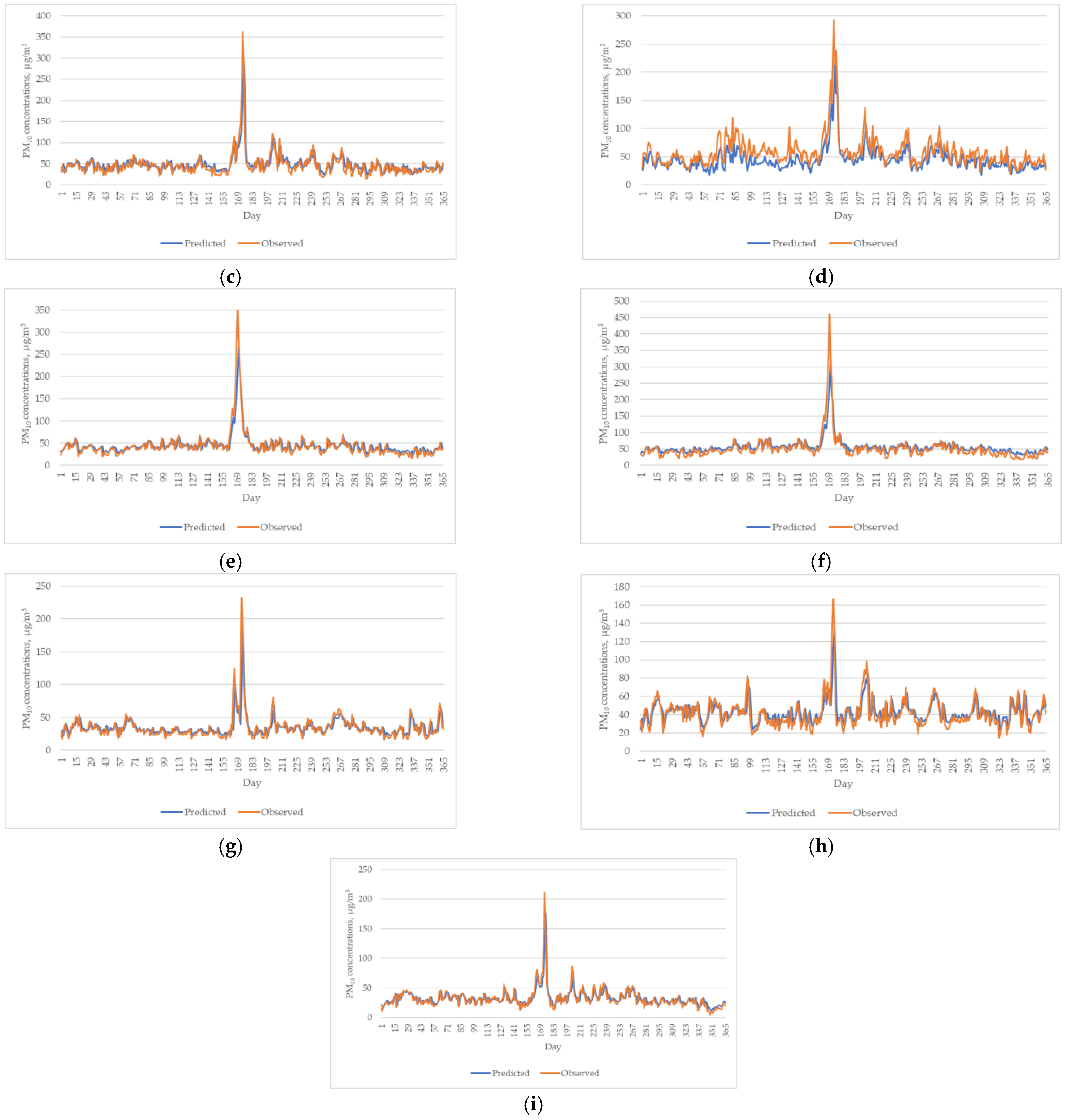
Overall, the BMA model is capable of making accurate estimates of the PM₁₀ concentrations for all monitoring stations, with the IA ranging from 0.884 to 0.907 and the rate of R² ranging from 63% to 75%. The BMA model obtained from the Pasir Gudang can be considered the most reliable model, followed by those obtained from the Kota Bharu and Larkin monitoring stations. Figure 15 shows the plot of predicted and observed PM₁₀ levels for all study areas. Generally, the BMA model successfully predicted the next-day PM₁₀ concentrations for all study areas. It can be seen that the predicted PM₁₀ concentration is capable of mimicking the variation of observed PM₁₀. However, the BMA model is observed to slightly underestimate the PM₁₀ level in Nilai and overestimate it in Kangar. The capacity of the models to make accurate forecasts changed depending on the quantities of pollution. In order to take into consideration the uncertainty associated with the models, BMA computes a weighted average for the quantity of interest based on a subset of all possible models that has been predetermined [48]. One of the benefits of using BMA is that it allows all predictor variables to be included in the model; however, the variables that are less important have smaller weights. The posterior probability can be interpreted for posterior probability below 50%, and there is some evidence opposing the impact. This demonstrates that the high RMSE at Nilai in comparison to Jerantut was caused by pollution concentrations, which resulted in a drop in the model’s ability to accurately forecast outcomes. Table 11 provides a summary and overview of the findings from other researchers who used BMA for forecasting data pertaining to air pollution.

Figure 15. Predicted vs. observed PM₁₀ concentration in all study areas. (a) Kangar, (b) Perai, (c) Shah Alam, (d) Nilai, (e) Larkin, (f) Pasir Gudang, (g) Paka, (h) Kota Bharu and (i) Jerantut.

Table 11. An overview of BMA model performance from different researchers.

Case Study	Parameter and Data	Result
Northern China [50]	PM10, CO, NOx, temperature, relative humidity, wind speed and pressure (2009–2010)	- In the absence of information, the uniform distribution was used as a non-informative prior in the investigation. - The BMA + GAMM technique for single pollutant evaluates the influence of PM10 on daily respiratory death rate, with an increase in PM10 concentration equivalent to 0.87 % to 1.38 %. - The BMA could be useful for modelling uncertainty in time series studies.
Europe [51]	NO2, PM10 and SO2, number of fragments, shares of artificial, agricultural, wetland, forest areas, population density, population decentralization (2006)	- The optimum model specification was chosen by adding variables with posterior inclusion probabilities equal to or greater than 0.5. - The urban structure has a considerable impact on the concentration of pollution. - According to the BMA model, the proportion of agricultural, artificial areas and temperature all have a major impact on pollution concentration.
West Central, Scotland [44]	NO2, 2089 disease data (2006–2012)	- The BMA averaged the estimated effect sizes from the 42 models. - The calculated relative risk was 1.011. - Cardio-respiratory mortality rose by an estimated 1.1% for every 5 µg/m3 increase in NO2 concentrations. - The likelihood that the relative risk is greater than one is 0.884.
Portugal [84]	O3 and PM10 (July 2006)	- Various ensemble techniques, including the Median Ensemble (MED), Static Linear Regression (SLR), Dynamic Linear Regression (DLR) and BMA, were utilized and compared. - Improvements in RMSE and correlation coefficient for PM10 were 18% and 11%, respectively. - The same statistical analysis, combined with probabilistic metrics, revealed that the SLR and BMA approaches performed well.
Seoul, South Korea [85]	PM10, O3, NO2, CO and SO2 (2005–2015)	- The findings revealed that pneumonia was strongly linked to air pollution, with R2 = 0.46 for BMA and R2 = 0.51 for PCR. - The greater posterior probability was 0.47. PM10 concentrations were the major parameter linked with substantial health risk, with the maximum posterior inclusion probability ranging from 80.2% to 100% and a positive correlation coefficient (0.14 to 0.34). - The study found that BMA and PCR provided substantial results, as well as the reliability and usability of these procedures in the study.
Henan Province, China [52]	PM2.5, PM10, O3, NO2, CO and SO2 (2017–2019)	- CUACE, NAQP, and CMAQ pollutant concentration forecast performance in Henan Province, China. - For PM2.5 concentrations with a 24-h lead time, the RMSE of BMA dropped by 35, 37, 68 and 50 percent in winter, spring, summer and autumn relative to the CUACE model, while the normalised mean bias decreased by 67, 83, 94 and 55% for O3. - Compared with the CMAQ model, the RMSE of the SO2, NO2 and CO forecasts by BMA were reduced by 29, 33 and 39%, respectively. - The BMA-predicted concentrations of the six contaminants during a significant pollution event matched measurements.

Researchers such as Wang et al. [86] used BMA and ensemble learning (BMA-EL) for forecasting a hybrid wind power, which indicates that the hybrid wind power forecasting approach based on BMA-EL has very good forecasting performance. The approach that was suggested possesses a low overall error and a high dependability, and it is able to precisely and reliably anticipate a wide range of weather and power situations. From this findings, BMA model was made possible to estimate PM₁₀ concentrations in examinations of air quality.

BMA does have some limits, for example, if it is given an infinite amount of data, the Bayesian inference will pick one model as the true model [47]. The outcomes of BMA depend on the candidate models’ prior probabilities, which are commonly overlooked. Different approaches are feasible and will alter the outcomes. The most common assumption is that all candidate models are equally plausible a priori [87]. Models with several parameters may be given less prior weight than models with few parameters. As is usually the case in Bayesian inference, one may specify different prior model probabilities and examine the degree to which the BMA results are qualitatively robust to changes in the prior. This is a good thing if one of the models under consideration is the real model that makes the data [88]. If this is not the case, however, BMA will not find the right model. Model selection and averaging are not always about finding the true model. Instead, they are about finding the model that should trust the most given the assumptions. This last belief is supported by both the data and the models. BMA is particularly useful when researchers are interested in a particular parameter, but do not know exactly how this parameter relates to the observations. In other words, they are uncertain about the underlying model. Future research will incorporate seasonal data in the BMA model for training and forecasting, and BMA could be beneficial for modelling uncertainty in time series investigations.

4. Conclusions

The purpose of this work was to obtain predictions of PM₁₀ concentrations in Malaysia for a total of nine monitoring stations by employing a total of eight parameters including temperature, relative humidity, wind speed, NO₂, SO₂, CO and O₃. The data collected over the course of seventeen years of air monitoring, beginning in 1999 and continuing through 2015, served as the foundation for these forecasts. Some of the monitoring stations that are involved are Kangar, Perai, Shah Alam, Nilai, Larkin, Pasir Gudang, Paka, Kota Bharu and Jerantut. This investigation’s goal is to determine how accurately Bayesian model averaging (BMA) can anticipate the next-day PM₁₀ concentration. The relative humidity, the wind speed and the PM₁₀ concentrations were the most important parameters that contributed to the forecast model on that day for the majority of stations, as indicated by the BMA models. The BMA model works the best for the Pasir Gudang monitoring station with R² = 0.752. Furthermore, the BMA models demonstrated good prediction model performance, with an IA ranging from 0.84 to 0.91, R² ranging from 0.64 to 0.75 and KGE ranging from 0.61 to 0.74 for all monitoring stations. According to the results of the investigation, BMA should be utilised in research and forecasting operations pertaining to environmental issues such as air pollution. When comparing competing models, BMA ensures that uncertainty receives the attention it deserves, which, in the end, leads to more accurate forecasts. Particulate matter, particularly the dangerous PM₁₀ pollutant, must be forecasted during transboundary haze occurrences in order to determine and comprehend its dispersion behaviour in the atmosphere. This can give concerned citizens with information and raise their awareness to decrease outdoor activities in the impacted areas.

References

1. United Nations. Air Pollution and Air Climate Change. In Statistical Yearbook for Asia and the Pacific; UN ESCAP: Beirut, Lebanon, 2011; pp. 79–84. [Google Scholar]
2. Zhou, M.; Liu, Y.; Wang, L.; Kuang, X.; Xu, X.; Kan, H. Particulate Air Pollution and Mortality in a Cohort of Chinese Men. Environ. Pollut. 2014, 186, 1–6. [Google Scholar] [CrossRef] [PubMed]
3. Mohamed Noor, N.; Yahaya, A.S.; Abdullah, M.; Sandu, A.V. Variation of Air Pollutant (Particulate Matter-PM10) in Peninsular Malaysia Study in the Southwest Coast of Peninsular Malaysia. Rev. Chim. 2015, 66, 1443–1447. [Google Scholar]
4. Latif, M.T.; Dominick, D.; Ahamad, F.; Khan, M.F.; Juneng, L.; Hamzah, F.M.; Nadzir, M.S.M. Long Term Assessment of Air Quality from a Background Station on the Malaysian Peninsula. Sci. Total Environ. 2014, 482–483, 336–348. [Google Scholar] [CrossRef] [PubMed]
5. Jamalani, M.A.; Abdullah, A.M.; Azid, A.; Ramli, M.F.; Baharudin, M.R.; Chng, K.; Elhadi, R.E.; Yusof, K.M.K.K.; Gnadimzadeh, A.; Quality, A.; et al. PM10 emission inventory of industrial and road transport emission inventory of industrial and road transport vehicles in Klang Valley, Peninsular Malaysia. J. Fundam. Appl. Sci. 2018, 10, 313–324. [Google Scholar] [CrossRef]
6. Wang, L.; Shi, T.; Chen, H. Air Pollution and Infant Mortality: Evidence from China. Econ. Hum. Biol. 2023, 49, 101229. [Google Scholar] [CrossRef]
7. Azhari, A.; Halim, N.D.A.; Mohtar, A.A.A.; Aiyub, K.; Latif, M.T.; Ketzel, M. Evaluation and Prediction of PM10 and PM2.5 from Road Source Emissions in Kuala Lumpur City Centre. Sustainability 2021, 13, 5402. [Google Scholar] [CrossRef]
8. Carugno, M.; Consonni, D.; Randi, G.; Catelan, D.; Grisotto, L.; Bertazzi, P.A.; Biggeri, A.; Baccini, M. Air Pollution Exposure, Cause-Specific Deaths and Hospitalizations in a Highly Polluted Italian Region. Environ. Res. 2016, 147, 415–424. [Google Scholar] [CrossRef]
9. Zoran, M.A.; Savastru, R.S.; Savastru, D.M.; Tautan, M.N. Impacts of Exposure to Air Pollution, Radon and Climate Drivers on the COVID-19 Pandemic in Bucharest, Romania: A Time Series Study. Environ. Res. 2022, 212, 113437. [Google Scholar] [CrossRef]
10. Hassan, N.A.; Hashim, Z.; Hashim, J.H. Impact of Climate Change on Air Quality and Public Health in Urban Areas. Asia Pac. J. Public Health 2014, 28, 38S–48S. [Google Scholar] [CrossRef]
11. Samsuddin, N.A.C.; Khan, M.F.; Maulud, K.N.A.; Hamid, A.H.; Munna, F.T.; Rahim, M.A.A.; Latif, M.T.; Akhtaruzzaman, M. Local and Transboundary Factors’ Impacts on Trace Gases and Aerosol during Haze Episode in 2015 El Niño in Malaysia. Sci. Total Environ. 2018, 630, 1502–1514. [Google Scholar] [CrossRef]
12. Latif, M.T.; Othman, M.; Idris, N.; Juneng, L.; Abdullah, A.M.; Hamzah, W.P.; Khan, M.F.; Nik Sulaiman, N.M.; Jewaratnam, J.; Aghamohammadi, N.; et al. Impact of Regional Haze towards Air Quality in Malaysia: A Review. Atmos. Environ. 2018, 177, 28–44. [Google Scholar] [CrossRef]
13. Abdullah, S.; Ismail, M.; Ahmed, A.N.; Abdullah, A.M. Forecasting Particulate Matter Concentration Using Linear and Non-Linear Approaches for Air Quality Decision Support. Atmosphere 2019, 10, 667. [Google Scholar] [CrossRef]
14. Sulong, N.A.; Latif, M.T.; Khan, M.F.; Amil, N.; Ashfold, M.J.; Wahab, M.I.A.; Chan, K.M.; Sahani, M. Source Apportionment and Health Risk Assessment among Specific Age Groups during Haze and Non-Haze Episodes in Kuala Lumpur, Malaysia. Sci. Total Environ. 2017, 601–602, 556–570. [Google Scholar] [CrossRef]
15. Akenji, L.; Bengtsson, M. Making Sustainable Consumption and Production the Core of Sustainable Development Goals. Sustainability 2014, 6, 513–529. [Google Scholar] [CrossRef]
16. Said, Z.; Sharma, P.; Elavarasan, R.M.; Tiwari, A.K.; Rathod, M.K. Exploring the Specific Heat Capacity of Water-Based Hybrid Nanofluids for Solar Energy Applications: A Comparative Evaluation of Modern Ensemble Machine Learning Techniques. J. Energy Storage 2022, 54, 105230. [Google Scholar] [CrossRef]
17. Shaziayani, W.N.; Ahmat, H.; Razak, T.R.; Zainan Abidin, A.W.; Warris, S.N.; Asmat, A.; Noor, N.M.; Ul-Saufie, A.Z. A Novel Hybrid Model Combining the Support Vector Machine (SVM) and Boosted Regression Trees (BRT) Technique in Predicting PM10 Concentration. Atmosphere 2022, 13, 2046. [Google Scholar] [CrossRef]
18. Plocoste, T.; Laventure, S. Forecasting PM10 Concentrations in the Caribbean Area Using Machine Learning Models. Atmosphere 2023, 14, 134. [Google Scholar] [CrossRef]
19. Qiao, W.; Wang, Y.; Zhang, J.; Tian, W.; Tian, Y.; Yang, Q. An Innovative Coupled Model in View of Wavelet Transform for Predicting Short-Term PM10 Concentration. J. Environ. Manag. 2021, 289, 112438. [Google Scholar] [CrossRef]
20. Sudharshan, K.; Naveen, C.; Vishnuram, P.; Krishna Rao Kasagani, D.V.S.; Nastasi, B. Systematic Review on Impact of Different Irradiance Forecasting Techniques for Solar Energy Prediction. Energies 2022, 15, 6267. [Google Scholar] [CrossRef]
21. Dai, H.; Huang, G.; Zeng, H.; Yu, R. Haze Risk Assessment Based on Improved PCA-MEE and ISPO-LightGBM Model. Systems 2022, 10, 263. [Google Scholar] [CrossRef]
22. Dai, H.; Huang, G.; Zeng, H.; Zhou, F. PM2.5 Volatility Prediction by XGBoost-MLP Based on GARCH Models. J. Clean Prod. 2022, 356, 131898. [Google Scholar] [CrossRef]
23. Department of Statistics Malaysia. Monthly Statistical Bulletin Malaysia; Department of Statistics Malaysia: Putrajaya, Malaysia, 2018. [Google Scholar]
24. Ul-Saufie, A.Z.; Yahaya, A.S.; Ramli, N.A.; Hamid, H.A. PM10 Concentrations Short Term Prediction Using Feedforward Backpropagation and General Regression Neural Network in a Sub-Urban Area. J. Environ. Sci. Technol. 2015, 8, 59–73. [Google Scholar] [CrossRef]
25. Fong, S.Y.; Abdullah, S.; Ismail, M. Forecasting of Particulate Matter (PM10) Concentration Based on Gaseous Pollutants and Meteorological Factors for Different Monsoons of Urban Coastal Area in Terengganu. J. Sustain. Sci. Manag. Spec. Issue Number 2018, 5, 3–18. [Google Scholar]
26. Abdullah, S.; Ismail, M.; Fong, S.Y.; Mahfoodh, A.; Ahmed, A.N. Evaluation for Long Term PM10 Concentration Forecasting Using Multi Linear Regression (MLR) and Principal Component Regression (PCR) Models. Environ. Asia 2016, 9, 101–110. [Google Scholar] [CrossRef]
27. Dominick, D.; Juahir, H.; Latif, M.T.; Zain, S.M.; Aris, A.Z. Spatial Assessment of Air Quality Patterns in Malaysia Using Multivariate Analysis. Atmos. Environ. 2012, 60, 172–181. [Google Scholar] [CrossRef]
28. Ul-Saufie, A.Z.; Yahaya, A.S.; Ramli, N.A.; Rosaida, N.; Hamid, H.A. Future Daily PM10 Concentrations Prediction by Combining Regression Models and Feedforward Backpropagation Models with Principle Component Analysis (PCA). Atmos. Environ. 2013, 77, 621–630. [Google Scholar] [CrossRef]
29. Hamid, H.A. Probabilistic and Distribution Modelling for Predicting PM10 Concentration in Malaysia; Universiti Sains Malaysia: George Town, Malaysia, 2013. [Google Scholar]
30. Bozdağ, A.; Dokuz, Y.; Gökçek, Ö.B. Spatial Prediction of PM10 Concentration Using Machine Learning Algorithms in Ankara, Turkey. Environ. Pollut. 2020, 263, 114635. [Google Scholar] [CrossRef]
31. Kumar, K.; Pande, B.P. Air Pollution Prediction with Machine Learning: A Case Study of Indian Cities. Int. J. Environ. Sci. Technol. 2022, 1–16. [Google Scholar] [CrossRef]
32. Suleiman, A.; Tight, M.R.; Quinn, A.D. Hybrid Neural Networks and Boosted Regression Tree Models for Predicting Roadside Particulate Matter. Environ. Model. Assess. 2016, 21, 731–750. [Google Scholar] [CrossRef]
33. Qin, S.; Liu, F.; Wang, J.; Sun, B. Analysis and Forecasting of the Particulate Matter (PM) Concentration Levels over Four Major Cities of China Using Hybrid Models. Atmos. Environ. 2014, 98, 665–675. [Google Scholar] [CrossRef]
34. Shahraiyni, H.T.; Sodoudi, S. Statistical Modeling Approaches for PM10 Prediction in Urban Areas; A Review of 21st-Century Studies. Atmosphere 2016, 7, 15. [Google Scholar] [CrossRef]
35. Stadlober, E.; Hörmann, S.; Pfeiler, B. Quality and Performance of a PM10 Daily Forecasting Model. Atmos. Environ. 2008, 42, 1098–1109. [Google Scholar] [CrossRef]
36. Brunelli, U.; Piazza, V.; Pignato, L.; Sorbello, F.; Vitabile, S. Two-Days Ahead Prediction of Daily Maximum Concentrations of SO2, O3, PM10, NO2, CO in the Urban Area of Palermo, Italy. Atmos. Environ. 2007, 41, 2967–2995. [Google Scholar] [CrossRef]
37. Paschalidou, A.K.; Karakitsios, S.; Kleanthous, S.; Kassomenos, P.A. Forecasting Hourly PM10 Concentration in Cyprus through Artificial Neural Networks and Multiple Regression Models: Implications to Local Environmental Management. Environ. Sci. Pollut. Res. 2011, 18, 316–327. [Google Scholar] [CrossRef]
38. Baklanov, A.; Hänninen, O.; Slørdal, L.H.; Kukkonen, J.; Bjergene, N.; Fay, B.; Finardi, S.; Hoe, S.C.; Jantunen, M.; Karppinen, A.; et al. Integrated Systems for Forecasting Urban Meteorology, Air Pollution and Population Exposure. Atmos. Chem. Phys. 2007, 7, 855–874. [Google Scholar] [CrossRef]
39. Amini, S.M.; Parmeter, C.F. Bayesian Model Averaging in R. Comput. Stat. Data Anal. 2011, 56, 1–35. [Google Scholar] [CrossRef]
40. Lee, Y.S. Management of a Periodic-Review Inventory System Using Bayesian Model Averaging When New Marketing Efforts Are Made. Int. J. Prod. Econ. 2014, 158, 278–289. [Google Scholar] [CrossRef]
41. Gibbons, J.M.; Cox, G.M.; Wood, A.T.A.; Craigon, J.; Ramsden, S.J.; Tarsitano, D.; Crout, N.M.J. Applying Bayesian Model Averaging to Mechanistic Models: An Example and Comparison of Methods. Environ. Model. Softw. 2008, 23, 973–985. [Google Scholar] [CrossRef]
42. Zhang, W.; Yang, J. Forecasting Natural Gas Consumption in China by Bayesian Model Averaging. Energy Rep. 2015, 1, 216–220. [Google Scholar] [CrossRef]
43. Li, G.; Shi, J. Application of Bayesian Model Averaging in Modeling Long-Term Wind Speed Distributions. Renew. Energy 2010, 35, 1192–1202. [Google Scholar] [CrossRef]
44. Pannullo, F.; Lee, D.; Waclawski, E.; Leyland, A.H. How Robust Are the Estimated Effects of Air Pollution on Health? Accounting for Model Uncertainty Using Bayesian Model Averaging. Spat. Spatio-Temporal Epidemiol. 2016, 18, 53–62. [Google Scholar] [CrossRef] [PubMed]
45. Benke, K.K.; Lowell, K.E.; Hamilton, A.J. Parameter Uncertainty, Sensitivity Analysis and Prediction Error in a Water-Balance Hydrological Model. Math. Comput. Model. 2008, 47, 1134–1149. [Google Scholar] [CrossRef]
46. Fragoso, T.M.; Bertoli, W.; Louzada, F. Bayesian Model Averaging: A Systematic Review and Conceptual Classification. Int. Stat. Rev. 2018, 86, 1–28. [Google Scholar] [CrossRef]
47. Hinne, M.; Gronau, Q.F.; van den Bergh, D.; Wagenmakers, E.J. A Conceptual Introduction to Bayesian Model Averaging. Adv. Methods Pract. Psychol. Sci. 2020, 3, 200–215. [Google Scholar] [CrossRef]
48. Hoeting, J.A.; Madigan, D.; Raftery, A.E.; Volinsky, C.T. Bayesian Model Averaging: A Tutorial. Stat. Sci. 1999, 14, 382–417. [Google Scholar]
49. Monteiro, A.; Ribeiro, I.; Tchepel, O.; Sá, E.; Ferreira, J.; Carvalho, A.; Martins, V.; Strunk, A.; Galmarini, S.; Elbern, H.; et al. Bias Correction Techniques to Improve Air Quality Ensemble Predictions: Focus on O3 and PM Over Portugal. Environ. Model. Assess. 2013, 18, 533–546. [Google Scholar] [CrossRef]
50. Fang, X.; Li, R.; Kan, H.; Bottai, M.; Fang, F.; Cao, Y. Bayesian Model Averaging Method for Evaluating Associations between Air Pollution and Respiratory Mortality: A Time-Series Study. BMJ Open 2016, 6, e011487. [Google Scholar] [CrossRef]
51. Cárdenas Rodríguez, M.; Dupont-Courtade, L.; Oueslati, W. Air Pollution and Urban Structure Linkages: Evidence from European Cities. Renew. Sustain. Energy Rev. 2016, 53, 1–9. [Google Scholar] [CrossRef]
52. Qi, H.; Ma, S.; Chen, J.; Sun, J.; Wang, L.; Wang, N.; Wang, W.; Zhi, X.; Yang, H. Multi-Model Evaluation and Bayesian Model Averaging in Quantitative Air Quality Forecasting in Central China. Aerosol Air Qual. Res. 2022, 22, 210247. [Google Scholar] [CrossRef]
53. Evans, S. Bayesian Regression Analysis; University of Louisville: Louisville, KY, USA, 2012. [Google Scholar]
54. Ismail, A.S.; Abdullah, A.M.; Samah, M.A.A. Environmetric Study on Air Quality Pattern for Assessment in Northern Region of Peninsular Malaysia. J. Environ. Sci. Technol. 2017, 10, 186–196. [Google Scholar] [CrossRef]
55. Mohtar, Z.A.; Faizah, N.; Yusof, F.; Ramli, N.A.; Yahya, A.S. Comparison of Particulate Matter (PM10) Monitoring Using Beta Attenuation Monitor (BAM) and Simple Instrument. Int. J. Eng. Technol. 2013, 3, 358–367. [Google Scholar]
56. Mohd Zahid, A.Z.; Abdul Malik, N.N.A.; Kassim, J. Particulate Matter Study at Residential and Educational Areas in Shah Alam, Malaysia. MATEC Web Conf. 2018, 06010, 1–16. [Google Scholar] [CrossRef]
57. Ahmat, H. Prediction of PM10 Concentrations Using Extreme Value Distributions (EVD): Classical and Bayesian Approaches; Universiti Sains Malaysia: George Town, Malaysia, 2016. [Google Scholar]
58. Noor, N.M.; Abdullah, M.M.A.; Tan, C.Y.; Ramli, N.A.; Yahay, A.S.; Fitri, N.F.M.Y. Modelling of PM10 Concentration for Industrialized Area in Malaysia: A Case Study in Shah Alam. Phys. Procedia 2011, 22, 318–324. [Google Scholar] [CrossRef]
59. Amin, N.A.M.; Adam, M.B.; Aris, A.Z. Bayesian Extreme for Modeling High PM10 Concentration in Johor. Procedia Environ. Sci. 2015, 30, 309–314. [Google Scholar] [CrossRef]
60. AhmadIsiyaka, H.; Juahir, H.; Toriman, M.E.; Gasim, B.M.; Azid, A.; Amri, M.K.; Ibrahim, A.; Usman, U.N.; Rano, A.R.; Garba, M.A. Spatial Assessment of Air Pollution Index Using Environmetric Modeling Techniques. Adv. Environ. Biol. 2014, 8, 244–256. [Google Scholar]
61. Ismail, A.S.; Latif, M.T.; Azmi, S.Z.; Juneng, L.; Jemain, A.A. Variation of Surface Ozone Recorded at the Eastern Coastal Region of the Malaysian Peninsula. Am. J. Environ. Sci. 2010, 6, 560–569. [Google Scholar] [CrossRef]
62. Awang, N.R.; Elbayoumi, M.; Ramli, N.A.; Yahaya, A.S. The Influence of Spatial Variability of Critical Conversion Point (CCP) in Production of Ground Level Ozone in the Context of Tropical Climate. Aerosol Air Qual. Res. 2016, 16, 153–165. [Google Scholar] [CrossRef]
63. Banan, N.; Latif, M.T.; Juneng, L.; Ahamad, F. Characteristics of Surface Ozone Concentrations at Stations with Different Backgrounds in the Malaysian Peninsula. Aerosol Air Qual. Res. 2013, 13, 1090–1106. [Google Scholar] [CrossRef]
64. Awang, N.R.; Ramli, N.A.; Mohammed, N.I.; Yahaya, A.S. Time Series Evaluation of Ozone Concentrations in Malaysia Based on Location of Monitoring Stations Time Series Evaluation of Ozone Concentrations in Malaysia Based on Location of Monitoring Stations. Int. J. Eng. Technol. 2013, 3, 390–394. [Google Scholar]
65. Kery, M. Introduction to WinBUGS for Ecologists: A Bayesian Approach to Regression, ANOVA, Mixed Models and Related Analyses, 1st ed.; Elsevier Inc.: Amsterdam, The Netherlands, 2010; ISBN 978-0-12-378605-0. [Google Scholar]
66. Kruschke, J.K. Doing Bayesian Data Analysis: A Tutorial with R and BUGS, 1st ed.; Academic Press: Cambridge, MA, USA, 2010; ISBN 0123814855. [Google Scholar]
67. Leamer, E.E. Specification Searches: Ad Hoc Inference with Nonexperimental Data, 1st ed.; John Wiley & Sons: New York, NY, USA, 1978; ISBN 0471015202. [Google Scholar]
68. Tzikas, D.G.; Likas, A.C.; Galatsanos, N.P. The Variational Approximation for Bayesian Inference. IEEE Signal Process. Mag. 2008, 25, 131–146. [Google Scholar] [CrossRef]
69. Adrian Raftery, A.; Hoeting, J.; Volinsky, C.; Painter, I.; Yeung, K. Package “BMA”: Bayesian Model Averaging; 2015. Available online: https://cran.r-project.org/web/packages/BMA/BMA.pdf (accessed on 4 December 2020).
70. Amini, S.M.; Parmeter, C.F. Bayesian Model Averaging in R. J. Econ. Soc. Meas. 2011, 36, 253–287. [Google Scholar] [CrossRef]
71. Sloughter, J.M.; Gneiting, T.; Raftery, A.E. Probabilistic Wind Speed Forecasting Using Ensembles and Bayesian Model Averaging. J. Am. Stat. Assoc. 2010, 105, 25–35. [Google Scholar] [CrossRef]
72. Madigan, D.; Raftery, A.E. Model Selection and Accounting in Graphical Models for Model Uncertainty Using Occam’s Window. J. Am. Stat. Assoc. 1994, 89, 1535–1546. [Google Scholar] [CrossRef]
73. Department of Environment Malaysia. Malaysia Annual Report 2015; Department of Environment Malaysia: Putrajaya, Malaysia, 2015. [Google Scholar]
74. Department of Environment Malaysia. Malaysia Environmental Quality Report 2006; Department of Environment Malaysia: Putrajaya, Malaysia, 2007. [Google Scholar]
75. Department of Environment Malaysia. Malaysia Environmental Quality Report 2005; Department of Environment Malaysia: Putrajaya, Malaysia, 2006. [Google Scholar]
76. Afroz, R.; Hassan, M.N.; Ibrahim, N.A. Review of Air Pollution and Health Impacts in Malaysia. Environ. Res. 2003, 92, 71–77. [Google Scholar] [CrossRef]
77. Kamarul Zaman, N.A.F.; Kanniah, K.D.; Kaskaoutis, D.G. Estimating Particulate Matter Using Satellite Based Aerosol Optical Depth and Meteorological Variables in Malaysia. Atmos. Res. 2017, 193, 142–162. [Google Scholar] [CrossRef]
78. Department of Environment Malaysia Chronology of Haze Episodes in Malaysia. Available online: www.doe.gov.my/en/2021/10/26/chronology-of-haze-episodes-in-malaysia-2/ (accessed on 15 January 2022).
79. Rahman, A.S.R.; Ismail, S.N.S.; Ramli, M.F.; Latif, M.T.; Abidin, E.Z.; Praveena, S.M. The Assessment of Ambient Air Pollution Trend in Klang Valley. World Environ. 2015, 5, 1–11. [Google Scholar] [CrossRef]
80. Elbayoumi, M.; Ramli, N.A.; Yusof, N.F.F.; Yahaya, A.S.; Al Madhoun, W.; Ul-Saufie, A.Z. Multivariate Methods for Indoor PM10 and PM2.5 Modelling in Naturally Ventilated Schools Buildings. Atmos. Environ. 2014, 94, 11–21. [Google Scholar] [CrossRef]
81. Wong, Y.K.; Mohamed Noor, N.; Mohamad Hashim, N.I. Temporal Variation of Ambient PM10 Concentration within an Urban-Industrial Environment. In Proceedings of the E3S Web of Conferences, Penang, Malaysia, 19 March 2018; EDP Sciences: Les Ulis, France, 2018; Volume 34. [Google Scholar]
82. Kusumaningtyas, S.D.A.; Aldrian, E. Impact of the June 2013 Riau Province Sumatera Smoke Haze Event on Regional Air Pollution. Environ. Res. Lett. 2016, 11, 075007. [Google Scholar] [CrossRef]
83. Yang, Q.; Yuan, Q.; Li, T.; Shen, H.; Zhang, L. The Relationships between PM2.5 and Meteorological Factors in China: Seasonal and Regional Variations. Int. J. Environ. Res. Public Health 2017, 14, 1510. [Google Scholar] [CrossRef]
84. Monteiro, A.; Ribeiro, I.; Tchepel, O.; Carvalho, A.; Martins, H.; Sá, E.; Ferreira, J.; Martins, V.; Galmarini, S.; Miranda, A.I.; et al. Ensemble Techniques to Improve Air Quality Assessment: Focus on O3 and PM. Environ. Model. Assess. 2013, 18, 249–257. [Google Scholar] [CrossRef]
85. Tran, H.; Kim, J.; Kim, D.; Choi, M.; Choi, M. Impact of Air Pollution on Cause-Specific Mortality in Korea: Results from Bayesian Model Averaging and Principle Component Regression Approaches. Sci. Total Environ. 2018, 636, 1020–1031. [Google Scholar] [CrossRef]
86. Wang, G.; Jia, R.; Liu, J.; Zhang, H. A Hybrid Wind Power Forecasting Approach Based on Bayesian Model Averaging and Ensemble Learning. Renew. Energy 2020, 145, 2426–2434. [Google Scholar] [CrossRef]
87. Consonni, G.; Fouskakis, D.; Liseo, B.; Ntzoufras, I. Prior Distributions for Objective Bayesian Analysis. Bayesian Anal. 2018, 13, 627–679. [Google Scholar] [CrossRef]
88. Vehtari, A.; Simpson, D.P.; Yao, Y.; Gelman, A. Limitations of “Limitations of Bayesian Leave-One-out Cross-Validation for Model Selection. ” Comput. Brain Behav. 2019, 2, 22–27. [Google Scholar] [CrossRef]
Disclaimer/Publisher’s Note: The statements, opinions and data contained in all publications are solely those of the individual author(s) and contributor(s) and not of MDPI and/or the editor(s). MDPI and/or the editor(s) disclaim responsibility for any injury to people or property resulting from any ideas, methods, instructions or products referred to in the content.
Article Metrics
Citations
Article Access Statistics
Multiple requests from the same IP address are counted as one view.