Simulations of Summertime Ozone and PM_2.5 Pollution in Fenwei Plain (FWP) Using the WRF-Chem Model

Abstract

In recent years, ozone and PM${}_{2.5}$ pollution has often occured in the Fenwei Plain due to heavy emission and favorable geographical conditions. In this study, we used the weather research and forecasting/chemistry (WRF-Chem) model to reproduce the complex air pollution of the ozone and PM${}_{2.5}$ in the Fenwei Plain (FWP) from 20 May to 29 May 2015. By comparing the simulation results with the observed data, we found that although in some cities there was a bias between the simulated values and observed data, the model captured the trend of pollutants generally. Moreover, according to the assessment parameters, we validated that the deviations are acceptable. However, according to these parameters, we found that the WRF-Chem performed better on ozone simulation rather than PM${}_{2.5}$. Based on the validation, we further analyzed the pollutant distribution during the contaminated period. Generally speaking, the polluted area is mainly located in the cities of the Shanxi province and Henan province. Moreover, in this time period, pollution mainly occurred on 27 May and 28 May. In addition, due to different formation conditions of ozone and PM${}_{2.5}$ pollution, the distribution characteristics of these two pollutants were also found to be different. Ozone pollution mainly occurred north of FWP due to the prevailing wind and the chemistry of ozone production. As for PM${}_{2.5}$, the pollution occurred at night and the polluted area was located in the FWP. Furthermore, high PM${}_{2.5}$ areas were closed to emission sources in the FWP, showing a high correlation with primary emissions.

1. Introduction

In China, pollutants including ozone and PM${}_{2.5}$ (particulate matter with aerodynamic diameter ≤ 2.5 $\mathsf{\mu }$m) can both affect air quality and cause serious pollution. Rapidly developing city clusters including the Yangtze River Delta, Pearl River Delta, North China Plain, and Fenwei Plain all face heavy ozone pollution in the summer and severe haze pollution in the autumn and winter [1,2]. Surface ozone is related to climate change and atmospheric oxidation, and surface PM${}_{2.5}$ is linked to atmospheric visibility. Moreover, these two pollutants both harm human health. In recent years, ozone and PM${}_{2.5}$ pollution often occur at the same time, and these two pollutants sometimes show a positive correlation in summertime [3,4].

Previous studies have investigated the characteristics of ozone and PM${}_{2.5}$ pollution in China. Deng et al. [2] concluded that annual mean ozone and PM${}_{2.5}$ concentrations show significant spatial clustering characteristics; the substantial increase of ozone mainly occurs in Beijing–Tianjin–Hebei (BTH), the Yangtze River midstream urban cluster (YRMR), Yangtze River Delta (YRD), and Pearl River Delta (PRD). As for high-level PM${}_{2.5}$ pollution, it was observed mainly in BTH, Fenwei Plain (FWP), the northern slope of the Tianshan Mountains urban cluster (NSTM), Sichuan Basin (SCB), and YRD. These polluted areas mentioned above are characterized by large emissions and favorable terrains for pollutant accumulations. In addition, the air pollution is closely related to meteorological conditions. Ozone pollution in China is usually accompanied with high temperatures, low wind speeds, and low relative humidity; PM${}_{2.5}$ pollution is accompanied by surface temperature inversion, low wind speed, high relative humidity, and low temperatures [5,6,7]. In addition, there are interactions between the ozone and PM${}_{2.5}$. On the one hand, photochemical processes involving ozone can enhance the atmospheric oxidation, thus promoting the formation of secondary aerosol, which is an important composition of PM${}_{2.5}$ [4]. On the other hand, aerosol attenuates solar radiation effectively and thus reduces ozone-related photochemical reaction rates [8].

The weather research and forecasting with chemistry model (WRF-Chem) is one of the numerical models that is commonly applied in ozone simulations in China [9,10,11]. Due to its high correlation coefficient and low bias with observed data, ozone simulation by WRF-Chem is credible and can be used for further research. Furthermore, WRF-Chem has been widely used for studying the temporal and spatial variation of aerosols; the PM${}_{2.5}$ simulation is dependable, but it does not perform as well as ozone simulation, and the overestimation of nitrate concentration and the simulated PBL mixing at night of the model are probable reasons [12,13,14]. In previous studies, WRF-Chem has been employed to predict meteorological conditions and pollutants in China to investigate the causes for the pollution formation. In general, studies have mainly focused on meteorological conditions and anthropogenic emissions. For instance, in the study of pollution in North China based on model results, Lv et al. [7] indicated that meteorological parameters, including relative humidity (RH) and wind speed, accounted for 47.8% of pollution. In addition, it is suggested that anthropogenic emission and PBL mixing intensity also play important roles in simulating the diurnal variation of pollutants [15]. However, most of the existing studies focused on areas with key air quality problems such as the North China Plain, and few studies focus on pollution characteristics and causes in the Fenwei Plain [5,16].

Fenwei Plain (FWP), a region with a large population, is one of the most polluted city clusters in China [17]. FWP is located in a coal-based area in Northern China and combines Fenhe Plain, Weihe Plain, and the surrounding terrace in the Yellow River Basin. FWP contains twelve cities in the Shanxi province, Henan province, and Shaanxi province. In FWP, contaminants and precursors of coal industry mainly come from cities in the Shanxi province and are the largest contributor to local VOCs [5,18]. Numerical simulations of pollutions in FWP are also limited. In addition, most of the previous studies based on WRF-Chem model mainly focused on the spatial distribution and seasonal variation of pollutants in urban clusters with key air quality problems in China such as North China Plain. Very few studies focused on the model performance of simulating the variation of ozone and PM${}_{2.5}$ during the complex pollution of the two pollutants. In order to address this issue, in this study, we employed WRF-Chem to investigate the performance of the model in simulating the complex air pollution in FWP. Furthermore, we also explored the characteristics of ozone and PM${}_{2.5}$ pollution occurring in FWP in May 2015. Deng et al. [19] has indicated that pollution in FWP shows a trend of contiguous spreading, which may be closely related to the coal-energy dominated consumption structure in FWP. Thus, the production of pollutants in FWP is driven by anthropogenic emissions and natural conditions such as local climate and topography, which are also influence factors that this study focuses on. This study can improve the understanding of the air pollution in FWP, and helps provide ideas for future research.

In Section 2, we describe the observed data and assessment parameters we used and the model configurations, including physical parameterization schemes and gas-phase mechanism. In Section 3 we evaluate the model performance in simulating meteorological parameters and pollutant concentrations. Furthermore, we analyze the model results to investigate pollution characteristics to find out the causes of the pollution. Finally, in Section 4, we list the major conclusions and prospects for future work.

2. Methodology

In this study, we selected a period from 20 May to 29 May 2015 to investigate the pollution in FWP. During this period, based on the observed pollutant concentrations, ozone in most cities in FWP was high, and PM${}_{2.5}$ was also high in cities such as Luoyang, Yuncheng, Jinzhong, Sanmenxia, and Lvliang. We employed the weather research and forecasting/chemistry (WRF-Chem) model to simulate the pollution episode. Then, the model results, including meteorological parameters and contaminants, were quantitatively evaluated by assessment parameters. After that, we analyzed the model results to discuss the pollution characteristics in FWP and explored the cause of pollution.

2.1. Observed Data

In this research, we used observed data of stations in cities in FWP to evaluate the model results. Cities located in FWP include Taiyuan (TY), Jinzhong (JZ), Lvliang (LL), Linfen (LF), Yuncheng (YC), Xi’an (XA), Baoji (BJ), Xianyang (XY), Weinan (WN), Tongchuan (TC), Luoyang (LY), and Sanmenxia (SMX), belonging to the Shanxi, Shaanxi and Henan provinces. The locations of these cities are listed in

Table 1. Locations of cities in Fenwei Plain.

City	Longitude	Latitude
Taiyuan (TY)	112.50	37.80
Xi’an (XA)	108.90	34.27
Baoji (BJ)	107.15	34.38
Luoyang (LY)	112.44	34.70
Linfen (LF)	111.50	36.08
Yuncheng (YC)	110.97	35.03
Jinzhong (JZ)	112.75	37.68
Xianyang (XY)	108.07	34.28
Weinan (WN)	109.58	34.95
Tongchuan (TC)	108.93	34.90
Sanmenxia (SMX)	111.19	34.76
Lvliang (LL)	111.12	37.51

and marked on Figure 1. We obtained the meteorological data (i.e., surface temperature, wind speed, and wind direction) of these cities from the National Climate Data Center (https://www.ncdc.noaa.gov/, accessed on 4 December 2022) [20]. The time resolution of meteorological parameters is one hour in TY, LY, and XY, and three hours in JZ, LL, LF, YC, XA, BJ, WN, TC, and SMX. In addition, pollutant concentrations (i.e., ozone and PM${}_{2.5}$) were provided by the National Urban Air Quality Real-time Release Platform of China Environmental Monitoring Station (http://www.cnemc.cn/, accessed on 4 December 2022) [21]. The time resolution of pollutants was one hour in all twelve cities. By analyzing the contaminant variation of the cities in FWP, we found that from 20 May to 29 May 2015, the ozone was mostly high in the twelve cities under investigation, and in some cities, ozone pollution was accompanied with high-level PM${}_{2.5}$. Thus, we selected this polluted episode to study.

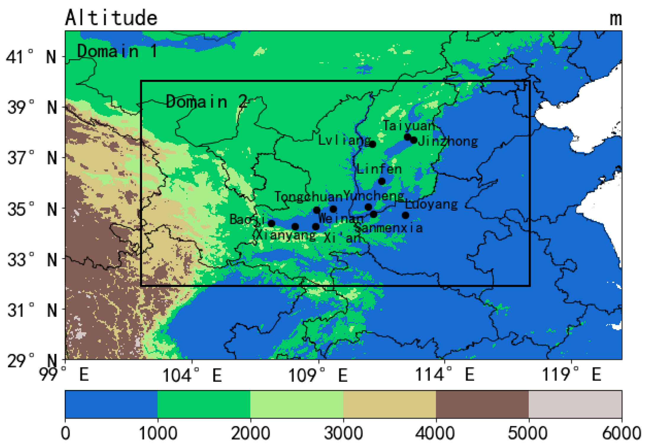
2.2. Model Configurations

In the study, we used version 3.9.1 of the weather research and forecasting/chemistry (WRF-Chem) model to reproduce the pollution in FWP. WRF-Chem was developed by research institutions including NOAA, DOE/PNNL, and NCAR [22]. WRF-Chem is a model which couples air quality and meteorological parameters, and it was confirmed to perform well on ozone prediction [23]. In the model, we set the simulation area on the Lambert projection and the center of the simulation area as 36.05° N, 110.02° E. As shown in Figure 1, we set two nested domains in the simulation. Domain 1 covers most of North China, and nested domain 2 covers FWP and the surrounding three provinces (Shanxi province, Shaanxi province, and Henan province). In the innermost domain, the simulation area has 214 grid points in the east-west direction, 145 grid points in the north-south direction, and 38 vertical layers. The physical parameterizations employed in this study are listed in

Table 2. Options used for parameterizations of atmospheric processes in the WRF-Chem model.

Process	Option	Reference
Cloud microphysics	Morrison 2-moment	Morrison et al. [24]
Longwave radiation	Rapid radiative transfer model (RRTM)	Mlawer et al. [25]
Shortwave radiation	Goddard	Chou et al. [26]
Surface layer	Monin–Obukhov scheme	Monin and Obukhov [27], Janić [28]
Land-surface physics	Noah land surface model	Chen and Dudhia [29], Ek et al. [30]
Urban surface physics	Urban canopy	Saijo et al. [31]
Planetary boundary layer	Yonsei University Scheme (YSU)	Hong et al. [32]
Cumulus parameterization	Grell 3D	Grell and Dévényi [33]

.

As for the simulation of chemical processes, we used the Statewide Air Pollution Research Center (SAPRC99) as the gas-phase mechanism, which has the ability to individually characterize the atmospheric reaction of 400 VOCs and estimate the reactivity of 550 VOCs [34]. Coupled with SAPRC99, we employed the model for simulating aerosol interactions and chemistry (MOSAIC) as the aerosol module, with a volatility basis set (VBS) of 8 sectional bins as the gas-particle distribution scheme. Moreover, to support the normal run of SAPRC99, the chemical mechanism is generated by the kinetic preprocessor (KPP), in which equations are solved using a Rosenbrock-type solver [35,36,37].

Due to the important role of meteorology in simulating pollutants, during the simulation, we employed a four-dimensional data assimilation (FDDA) to accurately reproduce the meteorological field by improving the initialization of the model. In the assimilation, we used the fifth generation ECMWR reanalysis data with the resolution of 0.25° × 0.25° as the initial field to drive the FDDA.

In the simulation, the anthropogenic emissions of pollutants (i.e., NOx, VOC, PM${}_{2.5}$, PM${}_{10}$) in the model were estimated by the 2015 emission inventory from the multi-resolution Emission Inventory for China (MEIC). In this emission inventory, emissions are classified as sectors of electricity, industry, civil society, transportation, and culture. Moreover, the temporal resolution of the emission data is monthly and the spatial resolution is 0.25°. As for the biological emissions, we used the model of emissions of gases and aerosols from nature (MEGAN), and it was calculated online based on weather and land-use data [38].

2.3. Assessment Parameters

To evaluate the model performance in predicting meteorological parameters and contaminants, we calculated the deviation between simulated results and observed data based on assessment parameters. The parameters applied in this study include correlation coefficient (R), index of agreement (IOA), mean bias (MB), and normalized mean bias (NMB). R, IOA, and MB were used to evaluate the simulated meteorological parameters, and R, IOA, and NMB were applied to validate the simulated pollutants [39,40]. Theses parameters were calculated as follows:

$$\mathrm{R}=\frac{{\sum }_{i=1}^n(P_i-\overline{P})(O_i-\overline{O})}{\sqrt{{\sum }_{i=1}^n{(P_i-\overline{P})}^2}\sqrt{{\sum }_{i=1}^n{(O_i-\overline{O})}^2}}$$

(1)

$$\mathrm{IOA}=1-\frac{{\sum }_{i=1}^n{(P_i-O_i)}^2}{{\sum }_{i=1}^n\left(\right|P_i-\overline{O}|+|O_i-\overline{O}{\left|\right)}^2}$$

(2)

$$\mathrm{MB}=\frac{{\sum }_{i=1}^n(P_i-O_i)}{n}$$

(3)

$$\mathrm{NMB}=\frac{{\sum }_{i=1}^n(P_i-O_i)}{{\sum }_{i=1}^n{O}_i}$$

(4)

In these formulas, n is the total number of data, P${}_i$ is the simulated value at the ith time point, and O${}_i$ is the observed value at the ith time point. $\overline{P}$ and $\overline{O}$ are time-averaged values in the simulations and observations, respectively.

3. Results and Discussion

We employed WRF-Chem to simulate the polluted episode from 20 May to 29 May 2015 to study the pollution in FWP. In this section, we evaluate the deviation between the simulated results and observed data and analyzed the pollution characteristics in FWP based on the simulated result.

3.1. Model Validation

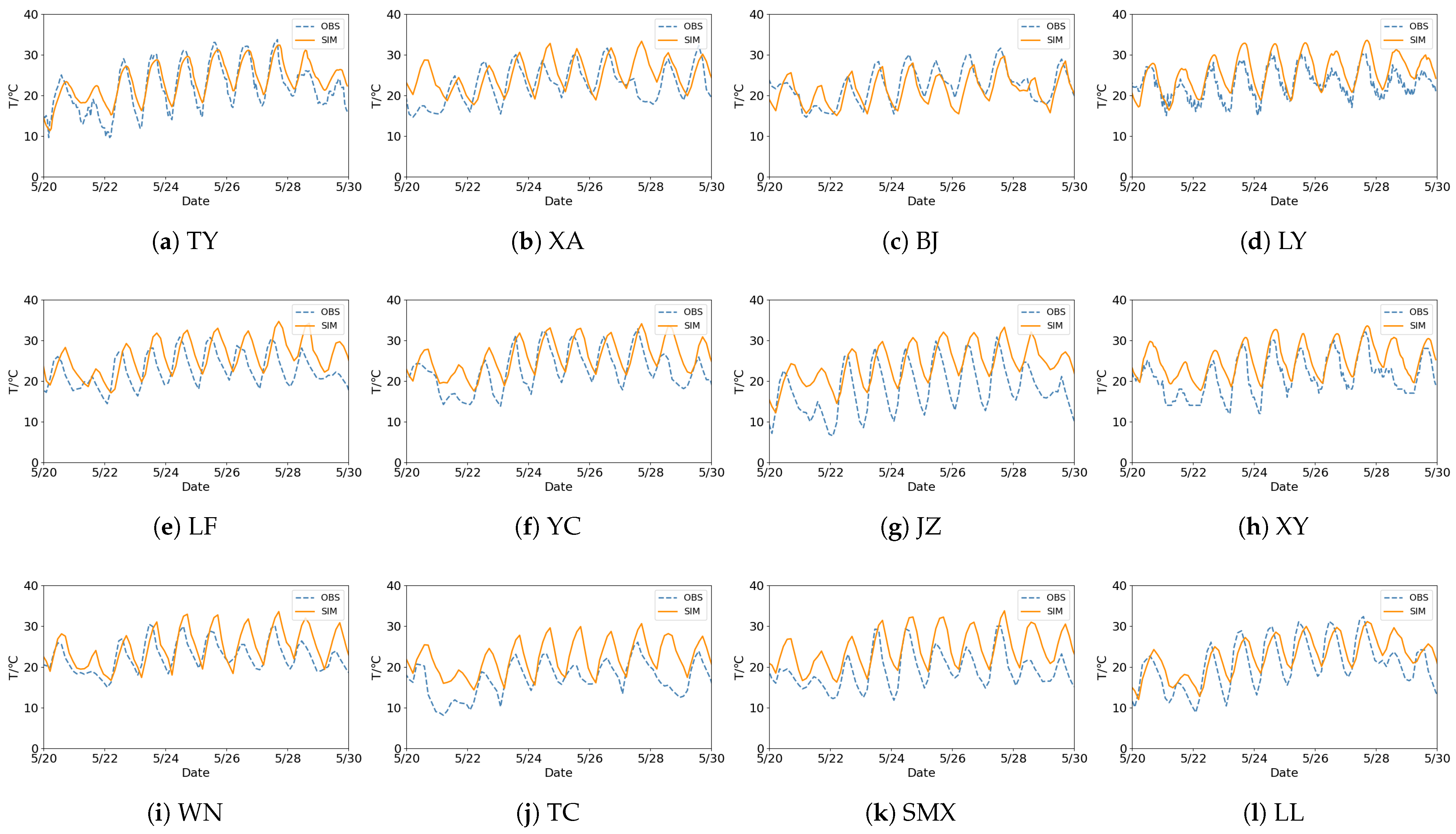
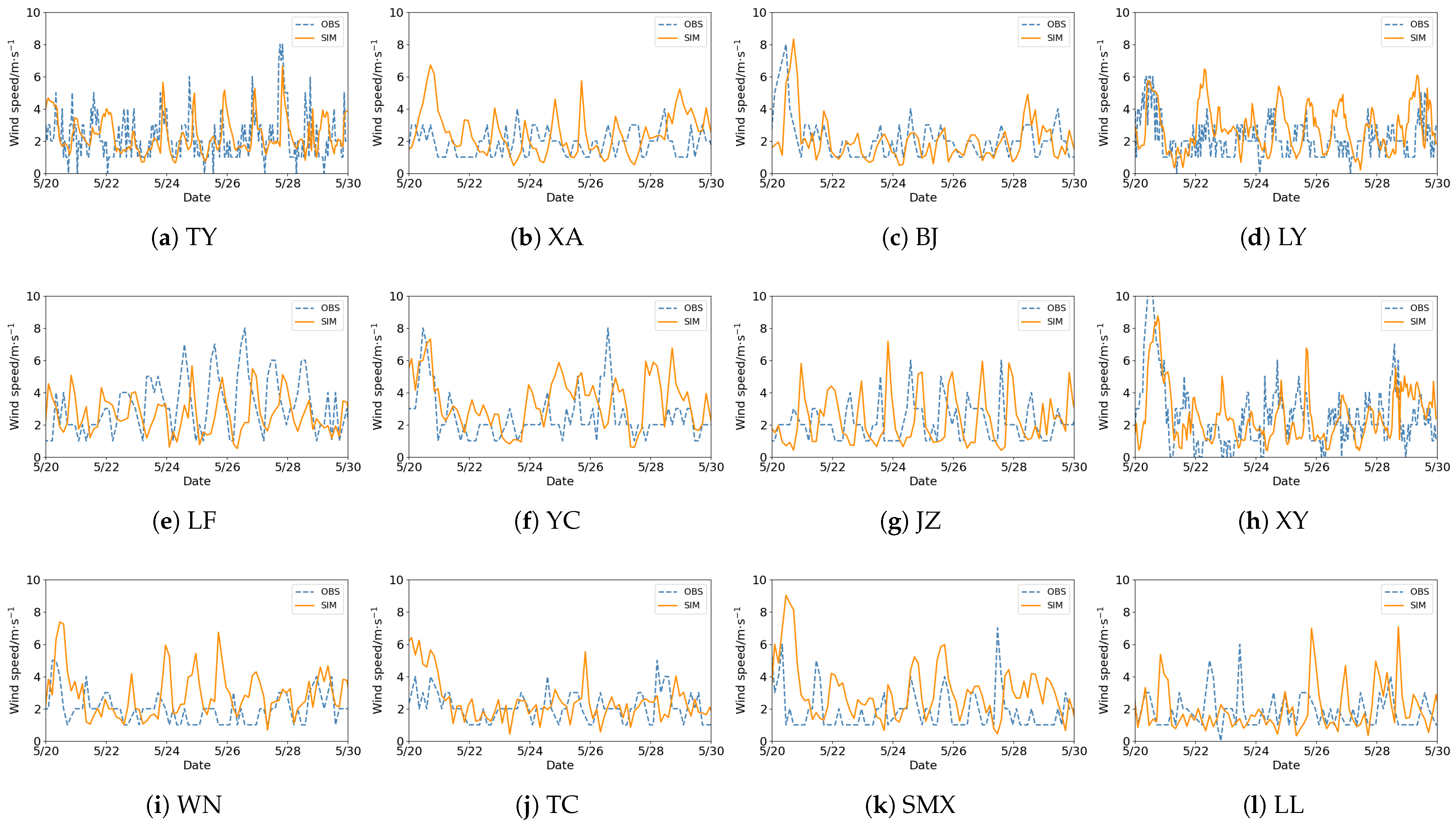
3.1.1. Simulated Meteorological Parameters

The variation of pollutant concentration is closely related to meteorological parameters such as temperature, wind speed, and wind direction. Thus, we applied the four-dimensional data assimilation (FDDA) to improve the prediction of meteorological parameters such as temperature and wind by the model. To validate the accuracy of pollutant results, we first compared the simulated results of meteorological parameters with the observed data. Figure 2 shows the model performance in simulating temperature at 2 m. It can be seen that in these cities in FWP, the observed maximum temperature in the afternoon reached a peak on 27 May and then began to decrease due to the precipitation. Based on the simulated results and assessment parameters, our model captured the change of temperature well, with high values of correlation coefficient (R) and index of agreement (IOA), indicating a high agreement between the simulated and observed results (see

Table 3. Assessment parameters for temperature predictions.

City	R	IOA	MB
Taiyuan (TY)	0.87	0.90	1.71
Xi’an (XA)	0.97	0.63	2.45
Baoji (BJ)	0.98	0.82	−1.11
Luoyang (LY)	0.77	0.78	2.70
Linfen (LF)	0.98	0.60	3.29
Yuncheng (YC)	0.97	0.71	3.33
Jinzhong (JZ)	0.93	0.62	6.00
Xianyang (XY)	0.80	0.74	3.96
Weinan (WN)	0.98	0.76	2.42
Tongchuan (TC)	0.96	0.61	5.10
Sanmenxia (SMX)	0.96	0.66	5.23
Lvliang (LL)	0.95	0.80	2.10

). Particularly, in XA, BJ, LF, YC, WN, and LL, the daily maximum and minimum values were both well reproduced, with R greater than 0.9 and MB less than 4.0. In addition, temperature results in LY and XY have a bias with the observed data. However, the biggest mean biases (MBs) in these cities are all within 6.0 and the R are all greater than 0.7, which means that the temperature simulation results are reliable, generally.

In addition to the temperature associated with photochemical reactions, we also validated the simulated wind speed and direction, which can heavily influence the pollutant dispersion. The comparison between the simulated wind and observed data is given in Figure 3. According to the observed wind, we found that wind speed values in this period in the twelve cities were all within 10 m·s${}^{-1}$, and the wind speed exhibited a significant diurnal variation. Based on the result comparison and the calculated parameters (see

Table 4. Assessment parameters for wind speed predictions.

City	R	IOA	MB
Taiyuan (TY)	0.25	0.55	0.06
Xi’an (XA)	0.69	0.23	0.56
Baoji (BJ)	0.74	0.56	−0.12
Luoyang (LY)	0.20	0.49	0.57
Linfen (LF)	0.73	0.39	−0.55
Yuncheng (YC)	0.80	0.55	0.90
Jinzhong (JZ)	0.60	0.25	0.16
Xianyang (XY)	0.46	0.69	−0.05
Weinan (WN)	0.77	0.39	0.89
Tongchuan (TC)	0.81	0.48	0.35
Sanmenxia (SMX)	0.64	0.35	1.07
Lvliang (LL)	0.61	0.30	0.12

), we found that the wind speed in BJ, LF, YC, WN, and TC was simulated relatively well, with R greater than 0.7 and MB less than 0.9. As for the result in TY, LY, and XY, we suggest that the bias might be caused by the one-hour monitoring interval, which is too fine, leading to the uncertainty of wind variation. In general, we believe that the simulated wind is also reliable in this study.

We then output the temporal variations of ozone and PM${}_{2.5}$ and calculated the assessment parameters between simulated and observed concentrations. In Figure 4, the observed ozone is high in the afternoon and reached a peak on 27 May in TY, XA, BJ, XY, TC, and SMX, and then began to decline, which is correlated with the change of temperature in Figure 2. In these cities of the FWP, hourly ozone reached up to 140 ppb in TY and XY on 27 May and formed high-level ozone pollution. Furthermore, except LL, the ozone exceeded up to 80 ppb during this period in another 9 cities and began to fall until 28 May. By comparing the observed and simulated ozone, we found that the model reproduced the variation of ozone during this period, and it both captured the trend and the peak value. However, we found that the model tended to underestimate ozone at night, which is maybe due to the difficulty in predicting the vertical profiles of ozone and NO${}_x$ at night [41]. Based on the assessment parameters (see

Table 5. Assessment parameters for ozone predictions.

City	R	IOA	NMB
Taiyuan (TY)	0.83	0.89	−0.15
Xi’an (XA)	0.40	0.61	0.39
Baoji (BJ)	0.37	0.58	0.36
Luoyang (LY)	0.63	0.78	−0.09
Linfen (LF)	0.44	0.49	0.94
Yuncheng (YC)	0.39	0.63	−0.06
Jinzhong (JZ)	0.79	0.88	−0.08
Xianyang (XY)	0.41	0.61	0.35
Weinan (WN)	0.34	0.56	0.46
Tongchuan (TC)	0.72	0.84	0.05
Sanmenxia (SMX)	0.35	0.6	0.12
Lvliang (LL)	0.78	0.64	0.81

), the model performed the best on ozone simulation in TY, with R of 0.83 and IOA of 0.89, which shows a high agreement with the observed data. Meanwhile, the simulated ozone in most of the other cities were also in good agreement with the measurements, with high R and IOA. Thus, although WRF-Chem predicted low levels of night-time ozone, we believe that the model results are credible.

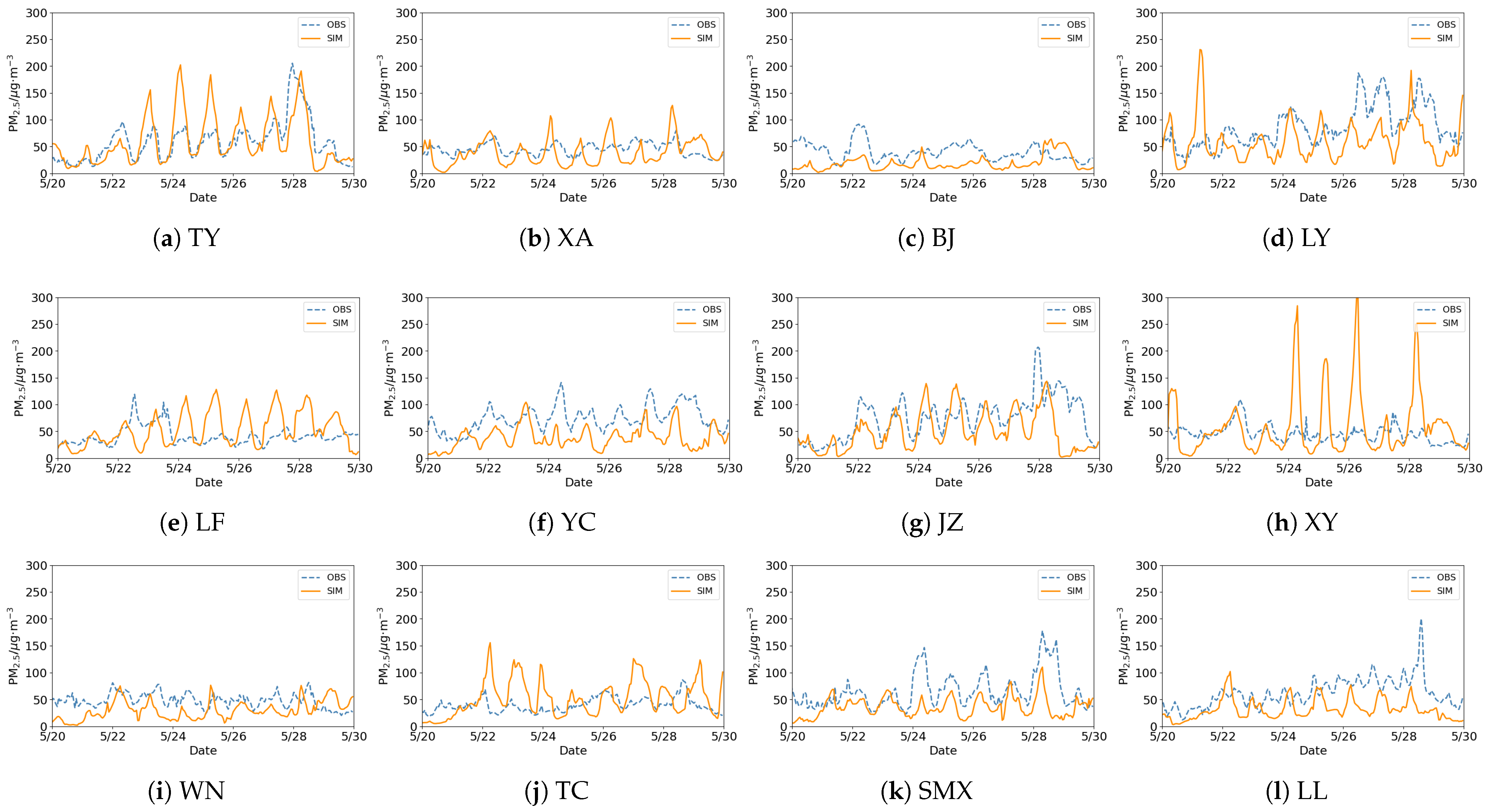
3.1.2. Simulated Pollutants

We also validated the simulated PM${}_{2.5}$ by comparing it to measurements and calculated the parameters. As shown in Figure 5, observed PM${}_{2.5}$ also shows an obvious diurnal behavior in heavily polluted cites such as TY, LY, YC, JZ, and SMX. In addition, in TY, LY, JZ, and SMX, high-level PM${}_{2.5}$ pollution occurred on 27 May and 28 May, and the concentrations exceeded 100 $\mathsf{\mu }$g·m${}^{-3}$ and reached up to 200 $\mathsf{\mu }$g·m${}^{-3}$ in TY and JZ. Dai et al. [42] indicated that the co-pollution of ozone and PM${}_{2.5}$ were often accompanied with high surface temperature. In this simulation, we found that the simulation results have the same rule and the peak values of pollutants and temperature appeared mainly from 27 May to 28 May. As for the simulated PM${}_{2.5}$, except BJ, the concentrations all show regular diurnal variation, which might be caused by the regularity of anthropogenic emission inventory we employed. Moreover, according to the comparison shown in Figure 5a–l, WRF-Chem tends to overestimate the peak concentration of PM${}_{2.5}$, but generally captured the variation of PM${}_{2.5}$. This may be due to the simulated high nitrate and low PBL height [12,13]. In

Table 6. Assessment parameters for PM${}_{2.5}$ predictions.

City	R	IOA	NMB
Taiyuan (TY)	0.66	0.79	0.02
Xi’an (XA)	0.24	0.47	−0.14
Baoji (BJ)	0.06	0.42	−0.54
Luoyang (LY)	0.23	0.49	−0.30
Linfen (LF)	0.05	0.29	0.25
Yuncheng (YC)	0.28	0.47	0.49
Jinzhong (JZ)	0.45	0.64	−0.34
Xianyang (XY)	0.07	0.20	0.29
Weinan (WN)	−0.07	0.32	−0.39
Tongchuan (TC)	0.06	0.30	0.30
Sanmenxia (SMX)	0.27	0.51	−0.46
Lvliang (LL)	0.33	0.52	−0.49

, the lower R and the higher MB show that the model performance of PM${}_{2.5}$ prediction is worse than that of the ozone. However, these parameters also demonstrate that the model performed well on PM${}_{2.5}$ prediction in TY, JZ, and LL.

The performances of WRF-Chem on simulating ozone and PM${}_{2.5}$ are quite different. Firstly, ozone is a secondary pollutant, which is generated by the reaction of precursors under solar radiation conditions. As for PM${}_{2.5}$, it contains emitted primary particles and secondary particles, and shows higher requirements on the emission inventory. Secondly, it has been proved that the gas-phase mechanism in WRF-Chem can predict ozone well, but there are problems with PM${}_{2.5}$ simulation, where it may overestimate the concentration of nitrate. What is more, because the PM pollution often occurs at night, the PM${}_{2.5}$ simulation is affected by the simulation of PBL mixing at night, and the underestimation of mixing intensity may lead to the overestimation of the peak value of the pollutant. However, the PBL mixing only influences the minimum night-time ozone concentration. In addition, the uncertainties in the gas-phase chemical mechanism, meteorological parameters, and emission inventory may also lead to biases in simulations [12,43].

3.2. Analysis of Pollution Distribution

In order to further explore the characteristics of ozone and PM${}_{2.5}$ pollutions in FWP, we continued to output the simulated distributions of pollutants in the innermost domain. We exhibited daily-averaged concentrations of ozone and PM${}_{2.5}$ during the heavily polluted period (i.e., 25 May to 28 May).

As shown in Figure 6, from 25 May to 28 May, FWP cities in the Shanxi province (TY, LF, YC, JZ, and LL) all experienced serious ozone pollution, and ozone in most areas in Shanxi exceeded 60 ppb, with the most severe areas (JZ, LF, and YC) exceeding 90 ppb. Due to the expansion of the contaminated area, pollution also occurred in the northern Henan cities on 26 May and in central Shaanxi cities on 27 May. Particularly, on 27 May, ozone concentration reached the peak and the polluted area reached its maximum extent, then ozone pollution influenced all cities in FWP. However, the ozone concentration on 28 May began to decrease due to the precipitation.

Combining the ozone distribution with the geographical condition shown in Figure 1, we found that ozone was not exactly concentrated in places with heavy emissions in FWP. In our simulations, high ozone was often found to be distributed both in the plain and the high-altitude regions, indicating that ozone pollution is not only related to anthropogenic emissions, but also affected by other factors such as meteorological conditions. For instance, in high-altitude areas, the solar radiation is relatively strong, which is favorable for ozone formation. In addition, during the Asia summer monsoon season (from May to September), wind fields in China are characterized by prevailing southwesterly-southeasterly winds, leading to the northward transportation of precursors and pollutants [44]. Meanwhile, due to the long lifetime of ozone in the troposphere, it can be affected by the wind field, being transported over long distances [45]. In general, being affected by the local chemistry, emissions, and meteorological conditions, the polluted area of ozone was not exactly located in places where the precursors are released in FWP, but was in fact further north.

As for the PM${}_{2.5}$ distribution shown in Figure 7, the PM${}_{2.5}$ pollution was relatively severe from 25 May to 28 May in FWP cities in Shanxi and Henan with a large polluted area, and PM${}_{2.5}$ exceeded 120 $\mathsf{\mu }$g·m${}^{-3}$ in heavily polluted areas. However, for cities in Shaanxi, the increase of PM${}_{2.5}$ was found to be delayed, occurring on 26 May, and the polluted area was relatively small, mainly located in XA (Xi’an) and XY (Xianyang).

Different from the ozone pollution we mentioned above, PM${}_{2.5}$ pollution mainly occurred in FWP and the North China Plain to the east of Shanxi. There are a large amount of pollution sources are located in these places, emitting primary pollutants and precursors of secondary pollutants. Generally speaking, pollution in FWP is influenced by local coal-based industry, and the polluted areas are close to emission sources [19]. In addition, as shown in Figure 5, high PM${}_{2.5}$ pollution in FWP cities occurred mainly at night, when the atmospheric boundary layer height is low and the turbulent mixing is weak. It is suggested that the PM${}_{2.5}$ simulation of WRF-Chem is primarily controlled by planetary boundary layer-mixing and emission variations [15]. Thus, at night, it is conducive to the local accumulation of pollutants, leading to the formation of PM pollution. Therefore, we suggest that the PM${}_{2.5}$ pollution in this period in FWP is mainly affected by anthropogenic primary emission and unfavorable diffusion conditions at night. In addition, as shown in Figure 7, the locations of many stations in these cities are close, so a small-scale pollution may have a large impact on simulations, leading to the bias of simulated results. This is also one of the possible reasons for the overestimation of pollutants in some cities we mentioned earlier.

4. Conclusions

In this study, we employed WRF-Chem to reproduce the ozone and PM${}_{2.5}$ pollution in FWP from 20 May to 29 May 2015. Based on the comparison of simulated results and the observed data, we found that WRF-Chem performed well on meteorological parameters and ozone concentration simulations; only the bias of PM${}_{2.5}$ simulation was larger than that of ozone. Based on the comparison of simulated results and observed data and the assessment parameters, we found the model results to be generally credible.

Furthermore, we investigated the distribution of pollutants based on the daily averaged pollutants from 25 May to 28 May 2015. During this period, ozone pollution first occurred in cities in the Shanxi province, and expanded to cities in Shaanxi and Henan. Moreover, ozone in cities with high altitude was at a similar level with that in other cities in FWP, indicating that ozone pollution is not only related to emission sources, but also affected by other meteorological and geographical conditions. In addition, due to the chemistry of ozone production and the prevailing wind in this period, the distribution of ozone was northerly to FWP. Different from the ozone, PM${}_{2.5}$ pollution in this time period mainly occurred in FWP. As we have mentioned, PM pollution always occurs at night, when the PBL condition is unfavorable to pollutant diffusion. Moreover, due to the economic structure in this area, there is a large amount of emission from the coal industry in FWP which contributes both primary particles and precursors of secondary particles that form PM${}_{2.5}$ pollution. Thus, PM${}_{2.5}$ in this period was mainly due to local emissions and weak diffusion conditions.

There are still some limitations in this study. For instance, the model performance on wind and PM${}_{2.5}$ simulations can be further improved by adjusting the boundary layer parameterization scheme. In addition, improving the understanding on air pollution in FWP is worthy of future study. To realize this purpose, we plan to simulate the variation of pollutant levels in different seasons in FWP. Moreover, we will adjust the model settings and select the appropriate parameterization scheme to obtain results that are reliable for further investigations.

References

1. Zong, L.; Yang, Y.; Gao, M.; Wang, H.; Gao, Z. Large-scale synoptic drivers of co-occurring summertime ozone and PM2.5 pollution in eastern China. Atmos. Chem. Phys. 2021, 21, 9105–9124. [Google Scholar] [CrossRef]
2. Deng, Y.; Inomata, S.; Sato, K.; Ramasamy, S.; Morino, Y.; Enami, S.; Tanimoto, H. Temperature and acidity dependence of secondary organic aerosol formation from α-pinene ozonolysis with a compact chamber system. Atmos. Chem. Phys. 2021, 21, 5983–6003. [Google Scholar]
3. Jia, M.; Zhao, T.; Cheng, X.; Gong, S.; Zhang, X.; Tang, L.; Liu, D.; Wu, X.; Wang, L.; Chen, Y. Inverse relations of PM2.5 and O3 in air compound pollution between cold and hot seasons over an urban area of east China. Atmosphere 2017, 8, 59. [Google Scholar] [CrossRef]
4. Li, J.; Cao, L.; Gao, W.; He, L.; Yan, Y.; He, Y.; Pan, Y.; Ji, D.; Liu, Z.; Wang, Y. Seasonal variations in the highly time-resolved aerosol composition, sources and chemical processes of background submicron particles in the North China Plain. Atmos. Chem. Phys. 2021, 21, 4521–4539. [Google Scholar] [CrossRef]
5. Wang, P.; Shen, J.; Xia, M.; Sun, S.; Zhang, Y.; Zhang, H.; Wang, X. Unexpected enhancement of ozone exposure and health risks during National Day in China. Atmos. Chem. Phys. 2021, 21, 10347–10356. [Google Scholar] [CrossRef]
6. Xie, B.; Zhang, H.; Wang, Z.; Zhao, S.; Fu, Q. A modeling study of effective radiative forcing and climate response due to tropospheric ozone. Adv. Atmos. Sci. 2016, 33, 819–828. [Google Scholar] [CrossRef]
7. Lv, Z.; Wei, W.; Cheng, S.; Han, X.; Wang, X. Meteorological characteristics within boundary layer and its influence on PM2.5 pollution in six cities of North China based on WRF-Chem. Atmos. Environ. 2020, 228, 117417. [Google Scholar] [CrossRef]
8. Ma, X.; Huang, J.; Zhao, T.; Liu, C.; Zhao, K.; Xing, J.; Xiao, W. Rapid increase in summer surface ozone over the North China Plain during 2013–2019: A side effect of particulate matter reduction control? Atmos. Chem. Phys. 2021, 21, 1–16. [Google Scholar] [CrossRef]
9. Dang, R.; Liao, H.; Fu, Y. Quantifying the anthropogenic and meteorological influences on summertime surface ozone in China over 2012–2017. Sci. Total Environ. 2021, 754, 142394. [Google Scholar] [CrossRef]
10. Ni, R.; Lin, J.; Yan, Y.; Lin, W. Foreign and domestic contributions to springtime ozone over China. Atmos. Chem. Phys. 2018, 18, 11447–11469. [Google Scholar]
11. Sun, L.; Xue, L.; Wang, Y.; Li, L.; Lin, J.; Ni, R.; Yan, Y.; Chen, L.; Li, J.; Zhang, Q.; et al. Impacts of meteorology and emissions on summertime surface ozone increases over central eastern China between 2003 and 2015. Atmos. Chem. Phys. 2019, 19, 1455–1469. [Google Scholar] [CrossRef]
12. Yang, J.; Zhao, Y. Performance and application of air quality models on ozone simulation in China—A review. Atmos. Environ. 2022, 293, 119446. [Google Scholar] [CrossRef]
13. Gao, M.; Carmichael, G.R.; Wang, Y.; Ji, D.; Liu, Z.; Wang, Z. Improving simulations of sulfate aerosols during winter haze over Northern China: The impacts of heterogeneous oxidation by NO2. Front. Environ. Sci. Eng. 2016, 10, 1–11. [Google Scholar] [CrossRef]
14. Fu, X.; Wang, S.; Chang, X.; Cai, S.; Xing, J.; Hao, J. Modeling analysis of secondary inorganic aerosols over China: Pollution characteristics, and meteorological and dust impacts. Sci. Rep. 2016, 6, 35992. [Google Scholar] [CrossRef] [PubMed]
15. Du, Q.; Zhao, C.; Zhang, M.; Dong, X.; Chen, Y.; Liu, Z.; Hu, Z.; Zhang, Q.; Li, Y.; Yuan, R.; et al. Modeling diurnal variation of surface PM2.5 concentrations over East China with WRF-Chem: Impacts from boundary-layer mixing and anthropogenic emission. Atmos. Chem. Phys. 2020, 20, 2839–2863. [Google Scholar] [CrossRef]
16. Akdi, Y.; Gölveren, E.; Ünlü, K.D.; Yücel, M.E. Modeling and forecasting of monthly PM2.5 emission of Paris by periodogram-based time series methodology. Environ. Monit. Assess. 2021, 193, 1–15. [Google Scholar] [CrossRef]
17. Bi, J.; Knowland, K.E.; Keller, C.A.; Liu, Y. Combining Machine Learning and Numerical Simulation for High-Resolution PM2.5 Concentration Forecast. Environ. Sci. Technol. 2022, 56, 1544–1556. [Google Scholar] [CrossRef]
18. Li, J.; Li, H.; He, Q.; Guo, L.; Zhang, H.; Yang, G.; Wang, Y.; Chai, F. Characteristics, sources and regional inter-transport of ambient volatile organic compounds in a city located downwind of several large coke production bases in China. Atmos. Environ. 2020, 233, 117573. [Google Scholar] [CrossRef]
19. Deng, C.; Tian, S.; Li, Z.; Li, K. Spatiotemporal characteristics of PM2.5 and ozone concentrations in Chinese urban clusters. Chemosphere 2022, 295, 133813. [Google Scholar] [CrossRef]
20. NOAA. National Centers for Environmental Information. Available online: https://www.ncdc.noaa.gov/ (accessed on 4 December 2022).
21. CNEMC. China National Environmental Monitoring Centre. Available online: http://www.cnemc.cn/ (accessed on 4 December 2022).
22. Mar, K.A.; Ojha, N.; Pozzer, A.; Butler, T.M. Ozone air quality simulations with WRF-Chem (v3. 5.1) over Europe: Model evaluation and chemical mechanism comparison. Geosci. Model. Dev. 2016, 9, 3699–3728. [Google Scholar] [CrossRef]
23. Grell, G.A.; Peckham, S.E.; Schmitz, R.; McKeen, S.A.; Frost, G.; Skamarock, W.C.; Eder, B. Fully coupled “online” chemistry within the WRF model. Atmos. Environ. 2005, 39, 6957–6975. [Google Scholar] [CrossRef]
24. Morrison, H.; Thompson, G.; Tatarskii, V. Impact of cloud microphysics on the development of trailing stratiform precipitation in a simulated squall line: Comparison of one-and two-moment schemes. Mon. Weather Rev. 2009, 137, 991–1007. [Google Scholar] [CrossRef] [Green Version]
25. Mlawer, E.J.; Taubman, S.J.; Brown, P.D.; Iacono, M.J.; Clough, S.A. Radiative transfer for inhomogeneous atmospheres: RRTM, a validated correlated-k model for the longwave. J. Geophys. Res.-Atmos. 1997, 102, 16663–16682. [Google Scholar] [CrossRef]
26. Chou, M.D.; Suarez, M.J.; Ho, C.H.; Yan, M.M.; Lee, K.T. Parameterizations for cloud overlapping and shortwave single-scattering properties for use in general circulation and cloud ensemble models. J. Clim. 1998, 11, 202–214. [Google Scholar] [CrossRef]
27. Monin, A.; Obukhov, A. Basic laws of turbulent mixing in the atmosphere near the ground. Tr. Geofiz. Inst. Akad. Nauk SSSR 1954, 24, 163–187. [Google Scholar]
28. Janić, Z.I. Nonsingular Implementation of the Mellor-Yamada Level 2.5 Scheme in the NCEP Meso Model; National Centers for Environmental Prediction: College Park, MD, USA, 2001.
29. Chen, F.; Dudhia, J. Coupling an advanced land surface–hydrology model with the Penn State–NCAR MM5 modeling system. Part I: Model implementation and sensitivity. Mon. Weather Rev. 2001, 129, 569–585. [Google Scholar] [CrossRef]
30. Ek, M.; Mitchell, K.; Lin, Y.; Rogers, E.; Grunmann, P.; Koren, V.; Gayno, G.; Tarpley, J. Implementation of Noah land surface model advances in the National Centers for Environmental Prediction operational mesoscale Eta model. J. Geophys. Res.-Atmos. 2003, 108, GCP12-1. [Google Scholar] [CrossRef]
31. Saijo, S.; Ikeda, S.; Yamabe, K.; Kakuta, S.; Ishigame, H.; Akitsu, A.; Fujikado, N.; Kusaka, T.; Kubo, S.; Chung, S.H.; et al. Dectin-2 recognition of α-mannans and induction of Th17 cell differentiation is essential for host defense against Candida albicans. Immunity 2010, 32, 681–691. [Google Scholar] [CrossRef]
32. Hong, S.Y.; Noh, Y.; Dudhia, J. A new vertical diffusion package with an explicit treatment of entrainment processes. Mon. Weather Rev. 2006, 134, 2318–2341. [Google Scholar] [CrossRef]
33. Grell, G.A.; Dévényi, D. A generalized approach to parameterizing convection combining ensemble and data assimilation techniques. Geophys. Res. Lett. 2002, 29, 38-1–38-4. [Google Scholar] [CrossRef]
34. Carter, W.P. Documentation of the SAPRC-99 chemical mechanism for VOC reactivity assessment. Contract 2000, 92, 95–308. [Google Scholar]
35. Damian, V.; Sandu, A.; Damian, M.; Potra, F.; Carmichael, G.R. The kinetic preprocessor KPP-a software environment for solving chemical kinetics. Comput. Chem. Eng. 2002, 26, 1567–1579. [Google Scholar] [CrossRef]
36. Sandu, A.; Daescu, D.N.; Carmichael, G.R. Direct and adjoint sensitivity analysis of chemical kinetic systems with KPP: Part I—Theory and software tools. Atmos. Environ. 2003, 37, 5083–5096. [Google Scholar] [CrossRef]
37. Sandu, A.; Sander, R. Simulating chemical systems in Fortran90 and Matlab with the Kinetic PreProcessor KPP-2.1. Atmos. Chem. Phys. 2006, 6, 187–195. [Google Scholar] [CrossRef] [Green Version]
38. Guenther, A.; Karl, T.; Harley, P.; Wiedinmyer, C.; Palmer, P.I.; Geron, C. Estimates of global terrestrial isoprene emissions using MEGAN (Model of Emissions of Gases and Aerosols from Nature). Atmos. Chem. Phys. 2006, 6, 3181–3210. [Google Scholar] [CrossRef]
39. Ding, H.; Cao, L.; Jiang, H.; Jia, W.; Chen, Y.; An, J. Influence on the Temperature Estimation by the Planetary Boundary Layer Scheme with Different Minimum Eddy Diffusivity in WRF v3. 9.1. 1. Geosci. Model. Dev. Discuss. 2021, 14, 6135–6153. [Google Scholar] [CrossRef]
40. Georgiou, G.K.; Christoudias, T.; Proestos, Y.; Kushta, J.; Pikridas, M.; Sciare, J.; Savvides, C.; Lelieveld, J. Evaluation of WRF-Chem model (v3. 9.1. 1) real-time air quality forecasts over the Eastern Mediterranean. Geosci. Model. Dev. 2022, 15, 4129–4146. [Google Scholar] [CrossRef]
41. Wei, W.; Lv, Z.F.; Li, Y.; Wang, L.T.; Cheng, S.; Liu, H. A WRF-Chem model study of the impact of VOCs emission of a huge petro-chemical industrial zone on the summertime ozone in Beijing, China. Atmos. Environ. 2018, 175, 44–53. [Google Scholar] [CrossRef]
42. Dai, H.; Zhu, J.; Liao, H.; Li, J.; Liang, M.; Yang, Y.; Yue, X. Co-occurrence of ozone and PM2. 5 pollution in the Yangtze River Delta over 2013–2019: Spatiotemporal distribution and meteorological conditions. Atmos. Res. 2021, 249, 105363. [Google Scholar] [CrossRef]
43. Shu, L.; Wang, T.; Han, H.; Xie, M.; Chen, P.; Li, M.; Wu, H. Summertime ozone pollution in the Yangtze River Delta of eastern China during 2013–2017: Synoptic impacts and source apportionment. Environ. Pollut. 2020, 257, 113631. [Google Scholar] [CrossRef]
44. Wu, J.; Bei, N.; Li, X.; Cao, J.; Feng, T.; Wang, Y.; Tie, X.; Li, G. Widespread air pollutants of the North China Plain during the Asian summer monsoon season: A case study. Atmos. Chem. Phys. 2018, 18, 8491–8504. [Google Scholar] [CrossRef]
45. Griffiths, P.T.; Murray, L.T.; Zeng, G.; Shin, Y.M.; Abraham, N.L.; Archibald, A.T.; Deushi, M.; Emmons, L.K.; Galbally, I.E.; Hassler, B.; et al. Tropospheric ozone in CMIP6 simulations. Atmos. Chem. Phys. 2021, 21, 4187–4218. [Google Scholar] [CrossRef]
Figure 1. The computational area and the nested domains used in the model. Stations possessing observed data were also marked by black points.
Atmosphere 14 00292 g001
Figure 2. The observed and predicted temperature at 2 m.
Atmosphere 14 00292 g002
Figure 3. The observed and predicted wind speed at 10 m.
Atmosphere 14 00292 g003
Figure 4. The observed and predicted concentrations of ozone.
Atmosphere 14 00292 g004
Figure 5. The observed and predicted concentrations of PM 2.5 .
Atmosphere 14 00292 g005
Figure 6. Spatial distributions of daily mean ozone on different days. Cities in Fenwei Plain are marked by blue circles.
Atmosphere 14 00292 g006
Figure 7. Spatial distributions of daily mean PM 2.5 on different days. Cities in Fenwei Plain are marked by blue circles.
Atmosphere 14 00292 g007