System of Imaging Photometers for Upper Atmospheric Phenomena Study in the Arctic Region

Abstract

A Pulsating Aurora Imaging Photometers Stereoscopic System (PAIPS) is suggested and described in the paper. The system is based on two lens telescopes with a matrix of multianode photomultiplier tubes as photodetectors placed in two high latitude observatories of the Polar Geophysical Institute. Telescopes provide simultaneous observations of a large volume of the atmosphere at altitudes in the range 50–100 km with high temporal resolution (up to 2.5 $\mathsf{\mu }$s) and a spatial resolution of about 2 km. This is a novel system for pulsating aurora study aimed to determine the energies of precipitating electrons responsible for the pulsating aurora occurrence. The system can be used for other atmospheric phenomena studies: meteors, transient luminous events, etc. One telescope has been operating since September 2021 and has measured a variety of optical phenomena.

1. Introduction

Pulsating aurora (PsA) is a type of diffuse luminescence of atmospheric gases stimulated by energetic electrons with quasiperiodic local changes in emission amplitude with periods from seconds to tens of seconds. The main pulsations that develop are in an on/off pattern. The typical size of PsA is in the range of 10–200 km and the typical altitude is around 100 km [1,2]. The altitude of PsA is determined by the energy of precipitating electrons and can vary in a wide range (see overview and discussion below).

PsAs can be classified on the basis of spatial structure: pure pulsations, expanding, streaming, propagating, etc. [3], or on the basis of temporal sequence (positive, negative, irregular and complex pulsations) [2]. Recently, a classification based on the stability of patches and the spatial extent of their pulsations was suggested by [4]. The authors identified the following types: Amorphous Pulsating Aurora (APA), Patchy Pulsating Aurora (PPA) and Patchy Aurora (PA). While APA is rapidly evolving pulsating features, PPA and PA are long-lived structures that can persist for tens of minutes, but PA does not pulsate. Interestingly, different types of aurora in this classification are mapped to various regions of the magnetosphere. PPAs and PAs are predominantly constrained between 4 and 9 $R_{\mathrm{E}}$, while a portion of the APA distribution maps to farther distances: as far out as ∼15 $R_{\mathrm{E}}$ [5].

It is well known that the temporal structure of PsA is even more complicated. The brightness of PsAs is characterized by a mixture of two periodical processes that co-exist hierarchically. In addition to the main pulsations, so-called “internal modulations” determine the temporal structure of emissions at a much higher frequency (∼3 Hz) [6]. There are not many detailed measurements of the temporal structure with high temporal resolution. Unusual, very fast fluctuations in pulsating auroras with an order of magnitude faster than the $3\pm 1$ Hz modulation were observed in [7]. These very high-frequency aurora emissions have not been explained yet.

The emission altitude of PsA is an important probe of precipitating electron energy. Therefore, the PsA altitude was studied both by optical methods, for example, by triangulation with all-sky video cameras, and by spectral methods. For example, in an early work [8], it was shown that PsA altitudes are in the range of 82–105 km with a median altitude of 92 km, which corresponds to the energy of electrons near 30 keV. In spectral methods, PsA’s altitude is derived from measurements of characteristic emission lines with different quenching altitudes and lifetimes. For example, in [9], a method using an excited O(${}^1$S) lifetime was proposed and later on applied in [10] for the statistical analyses of PsA altitudes. It was shown that altitudes are distributed in a range of 95–115 km, and it lowers significantly in the morning MLT sector, indicating the increase in precipitating electrons energy.

Previous measurements demonstrate that the energy of precipitating electrons varies in a wide range, starting from 1 keV [11]. The typical altitude of the PsA indicates that auroral pulsations are mostly generated by the precipitation of electrons with an energy of 20–40 keV. The interaction between magnetospheric electrons and VLF electromagnetic waves near the equator [12] is believed to cause these precipitations. A group of chorus waves scatters plasma sheet electrons into the loss cone [13]. Lower-band chorus waves are effective for higher energy electron ($E>7$ keV) precipitations, while upper-band chorus waves are more effective for energies below ∼3 keV [14].

The temporal structure of PsA also found its interpretation in the wave-particle interaction models. For example, the correlation of the internal modulation of PsA at a frequency near 3 Hz with discrete elements of chorus waves and electron flux at energies 10–30 keV was demonstrated by joint analyses of the ARASE satellite and ground-based optical observations [15]. The comparisons of ground-based observations of PsA taken by ultrafast auroral imagers and the electric field’s power spectral density measured by ARASE satellite in the magnetosphere showed a direct link between the morphology of PsAs and the characteristics of chorus waves [16].

On the other hand, the simulations in [17] demonstrate that microbursts of relativistic electrons arise during the interaction of chorus waves with particles, and these microbursts of relativistic electrons are the high-energy tail of pulsating aurora electrons. A strong correlation has recently been shown between microbursts of relativistic electrons and PAs [18].

Relativistic electrons precipitate much deeper into the atmosphere and create a higher level of ionization, up to 65 km ([19,20,21]), and change the chemistry of the mesosphere [22,23]. For this reason, a monitoring and detailed measurement of the low-altitude aurora emission produced by high-energy electrons is of great interest. Two highly sensitive photometers placed in two different locations will allow such kinds of triangulation and monitoring measurements to be conducted with a millisecond temporal resolution.

With the help of stereoscopic observations, it is possible to estimate the vertical emission profile, which means that the energy distribution of the precipitated particles (electrons) can be estimated, and the maximum energy of particles in a directed flux from the magnetosphere can be determined. Energetic electrons of magnetospheric origin rotate while moving along the magnetic field and, according to the configuration of the Earth’s magnetic field, fall into the upper layers at high latitudes. Collisional dissipation of energetic electrons in atmospheric gases leads to the generation of a cascade of secondary electrons and rapid isotropization of the electron flux. The depth of penetration into the gas target is determined by the passed mass and is uniquely found from the initial energy distribution of electrons in the beam by convolution with the dissipation function obtained early by Monte Carlo simulation [24]. A detailed simulation of monoenergetic electron beams penetration into the atmosphere was performed in [25] using a SIC (Sodänkyla Ion and Neutral Chemistry) model and the dependence of the ionization rate on energy and height is obtained. Recently, the Energetic Precipitation Monte Carlo (EPMC) model was developed and employed to calculate the ionization rate as a function of altitude produced by monoenergetic electrons [26]. The results of both simulations agree with each other and can be used for the primary particle energy reconstructions according to the height profile of the PsA emission. The profiles of the ionization rate obtained in [25] are shown in the left panel of Figure 1 to compare with proposed geometry of the experiment. The field of view (FOV) of the second photometer is optimized to measure the whole range of possible PsA emission altitudes, placing the high-energy electrons region in the center of the FOV.

Moreover, the statistical properties of the energy of PsA electrons are still unknown. Most studies use limited datasets. For example, [8] analyzed 2 h of measurements, and in [10], 37 nights of PsA events during 3 months from January to March 2018 were analyzed. The new Pulsating Aurora Imaging Photometers Stereoscopic (PAIPS) system designed in this work will operate continuously with 1 ms temporal resolution. The first photometer has been operating for 7 months (see below).

In what follows, we present the concept of measurements with the PAIPS system, description of the scientific equipment, its possible usage for various atmospheric phenomena observations and several examples of measurements conducted by the first photometer installed in Verkhnetulomsky observatory.

2. Instruments and Methods

The first imaging photometer of the PAIPS system was installed at the Verkhnetulomsky observatory (VTL, 68.63${}^{\circ }$ N, 31.78${}^{\circ }$ E) in September 2021 and made observations throughout the winter season until May 2022.

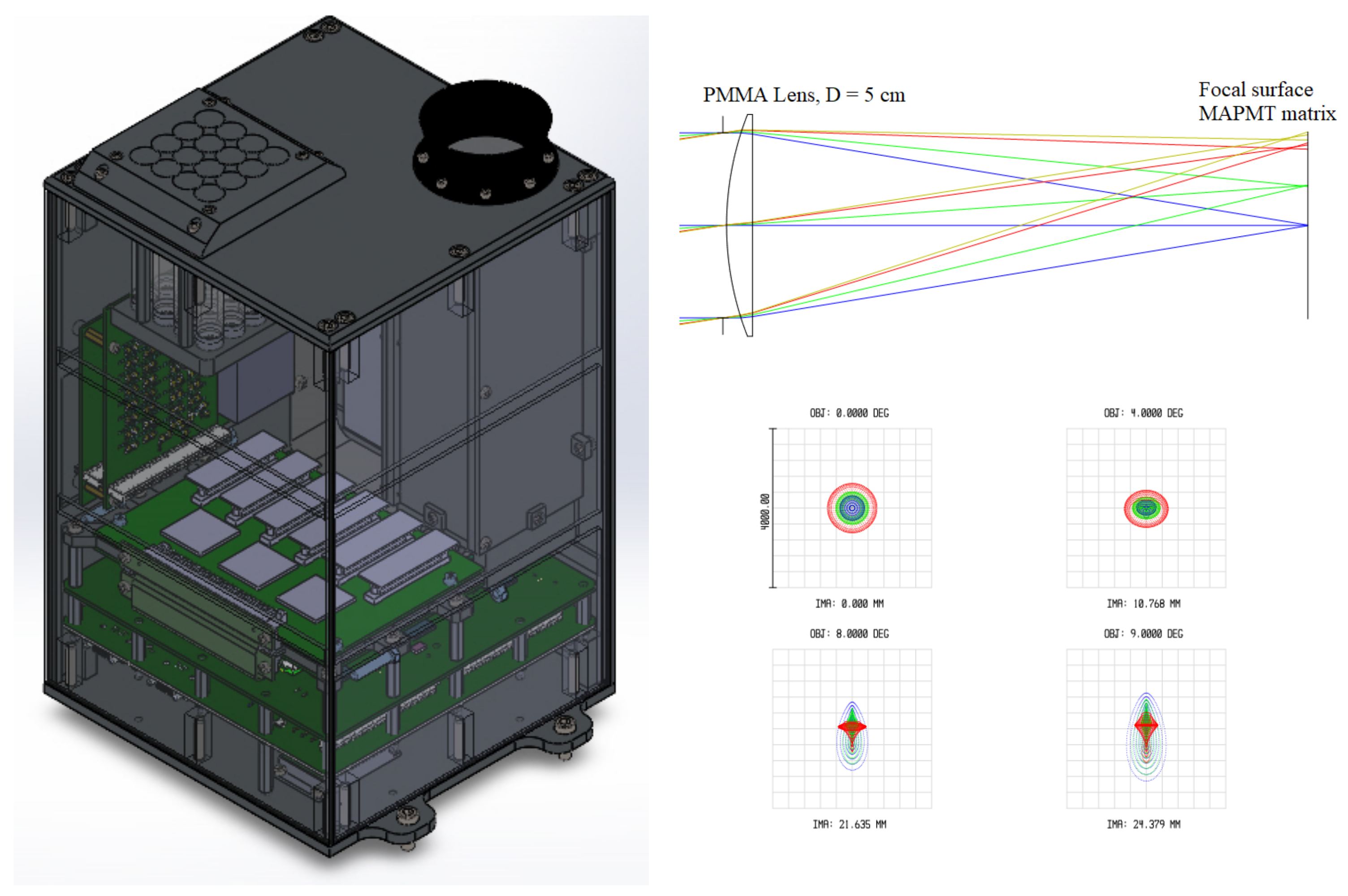
The imaging photometer is a simple lens telescope consisting of:

• an optical system in the form of a lens with a diameter of 5 cm (transparent in the near UV range: 300–400 nm);
• photodetector—a matrix of 4 multi-anode photomultiplier tubes (MAPMTs) ($16\times 16$ pixels, covered with BG3 filters transparent in the range of 300–400 nm);
• analog-to-digital conversion board based on specialized SPACIROC-3 microcircuits [27].

MAPMTs operate in a single photoelectron mode, which ensures the high sensitivity of the equipment. The structure of the photometer and the logic of its operation are similar to the Mini-EUSO telescope [28]. There are three operating modes working in parallel with different time resolutions: 2.5 $\mathsf{\mu }$s, 320 $\mathsf{\mu }$s and 41 ms. These modes allow phenomena of different duration and nature to be recorded.

Additionally, a spectrometer is installed in the photometer housing, which is a set of 16 single-channel PMTs with an analog electronics board. In front of each PMT there is a light filter that determines the wavelength range. The spectrometer operates in a direct current mode based on electronics similar to those implemented earlier in the TUS orbital experiment aboard the Lomonosov satellite [29]. The spectrometer is aimed to measure the characteristic lines of aurora emission to obtain additional information, which can be used for aurora altitude estimations (see discussion below). For the first years of operation, wide wavelength band filters UFS-1 (300–400 nm) and KS-11 (600–800 nm) will be used, as well as narrow filters with the 337 nm, 390 nm and 430 nm central wavelengths.

The photometer and spectrometer have a common digital data processing unit that provides event selection, recording to the internal DDR memory, control of operating modes and detector parameters, as well as an interface with a computer (the server for data storage).

The photometer and spectrometer have the same FOV. The spectrometer allows the measurement of the total radiation spectrum over the entire FOV, and the photometer—the localization of the emission source and its geometric shape.

In Figure 2, the 3D model of the detector is shown. The left part of the device is a 16-channel spectrometer, and the right part is an imaging photometer. A more detailed description of the photometer in the VTL is given in [30].

To carry out stereoscopic measurements, a second imaging photometer will be installed at the Lovozero observatory (LOZ, 67.98${}^{\circ }$ N, 35.01${}^{\circ }$ E). The photometer is also a lens telescope that makes it possible to obtain images of the objects, similar in functionality and registration methods to the first photometer, but with two essential modifications: increased sensitivity due to a larger area of the entrance window (the lens diameter will be increased from 5 to 20 cm, which will lower the threshold by more than an order of magnitude) and the addition of two identical measuring modules with 256 channels each, which will make it possible to observe almost the entire volume of the atmosphere above VTL.

The distance between the two observatories is 150 km; see Figure 3. The telescope at VTL has a FOV directed to the zenith, an angular resolution of about 1 degree, which provides a spatial resolution of about 2 km at the height of 100 km. The telescope at LOZ will be directed close to the horizon, and the field of view will be 0.5 rad to provide a view from 25 to 100 km in height above VTL. The angular resolution of the device, corresponding to a pixel of size $a=3$ mm and a focal length of the lens $f=30$ cm, will be 10 mrad. With such an angular resolution, the spatial resolution in height above VTL will be about 1.5 km. Details of the observation geometry can be seen in the right panel of Figure 1.

Such a system will make it possible to estimate the energy of precipitating particles by measuring the maximum emission depth of pulsating spatial structures.

Measurements of the emission spectrum provide an additional possibility to estimate the emission altitude. For this purpose, both instruments are equipped with fast spectrometers. Short-lived (70 ns) lines of the first negative nitrogen system (N2 + 1N): 391.4 and 427.8 nm are characteristic of the low emission height. The effective quenching altitude is 48 km. As shown in [31], about 0.6% of the energy of the MeV electron beam is released in these lines with maximum brightness at an altitude of about 60 km. More than 1% of the energy is released in the second positive system (N2 2PG), where the characteristic line with a short lifetime (50 ns) and low quenching altitude (30 km) is 337 nm, and more than 2% in the first positive system (N2 1PG) with relatively long lifetime (5 $\mathsf{\mu }$s) and effective quenching on molecular nitrogen up to a height of 53 km. Measurements of these lines and their ratios will make it possible to make an additional estimate of the emission altitude.

Photometric observations in the 557.7 and 630 nm lines will give an estimate of the soft part of the spectrum of precipitating electrons, and the 486 nm channel (H${}_{\beta }$) will give an estimate of the presence of proton precipitation. Absolute measurements of all observed emissions will be the basis for the verification of available models of the auroral ionosphere.

An important advantage of the equipment is the ability to register other atmospheric phenomena. In particular, due to the high temporal resolution and sensitivity, detailed recording of luminescence curves, selection and reconstruction of various track events are possible. Images moving along a linear track on a photodetector can be obtained from aircraft, satellites and meteors falling into the FOV. In addition, integrating the signal over several seconds reveals the movement of stars in the sky, and the curvature of the trajectory of which inside the FOV can be neglected in the first approximation.

Table 1. Ranges for different types of linear track objects and the optimal time resolution.

Object	Angular Velocity, $\mathsf{\Omega }$ (mrad/s)	Time Resolution, $\mathit{\tau }$ (ms)
Star	0.01–0.04	(5–10) $\times {10}^3$
Satellite	7–19	40–80
Plane	14–28 $(\sim$50)	20–40
Meteor	100–1000	1–2

shows the typical ranges of the angular velocities $\mathsf{\Omega }$ of these objects (as seen from the detector) and optimal time resolution $\tau$ to detect and analyze them.

To estimate the $\mathsf{\Omega }$ for the planes, we use the height of 10 km and speed of 500–1000 km/h, which are the typical values for civil aircraft. One can find that the Moscow–Murmansk curse goes through the VTL, and here (80 km from Murmansk), the plane is already lowering its altitude and speed before landing, so the typical value for $\mathsf{\Omega }$ is higher (indicated in parenthesis). A meteor is a relatively fast event, and for a detailed analysis (“fine-structure”) of its light curve, it is necessary to increase the time resolution to 1–2 ms.

Examples of track measurements from a passing satellite and meteor and their reconstruction by the LTA algorithm [32] are given in the next section. The LTA estimates the speed of movement of the image centroid along a rectilinear track, highlighting the active (above-threshold) part in the signal of each triggered channel and approximating the dependence of pixel coordinates on time with weights proportional to the values of the signal to some power by linear functions (the threshold value and the exponent are the control parameters of the algorithm). Examples of the application of the LTA method for the kinematic reconstruction of meteors are given in [33].

The most interesting and mysterious track events that can fall into the detector FOV are the so-called EAS-like events detected in the TUS experiment aboard the Lomonosov satellite, which can be both anthropogenic and astrophysical in nature [34,35]. These are definitely relativistic objects, and for triggering and analyzing them, a maximum resolution of the order of a microsecond is required.

3. Results and Discussion—Selected Examples of Measurements

As was mentioned above, the first photometer of PAIPS was installed in VTL in September 2021 and has measured a number of various phenomena. For the first year of observations, software developed earlier for the Mini-EUSO space experiment was used [36]. The main monitoring mode of the operation has a 41 ms temporal resolution. For future stereoscopic measurements, it will be increased to 1 ms. Some examples of the first year of measurements in the monitoring mode are presented below. Faster operation modes (2.5 and 320 $\mathsf{\mu }$s) are not considered in this paper.

3.1. Stars

In Figure 4, the pixel map measured on 8 December 2021 at 04:02:56 UTC is presented. It is placed on the top of the night sky image, which is seen at this time above VTL. Bright pixels in the FOV (yellow and green) correspond to stars. The two brightest are Dubhe (Alpha Ursae Majoris) with magnitude M = 1.79 and Kappa Draconis with M = 3.87. Less-bright stars in the left bottom corner of the pixel map also belong to the Ursa Major and have magnitudes of more than 4. A correspondence between telescope measurements and the position of stars is well seen. The size of the star image shows the rather good quality of the optical system. The central gaps in the image correspond to the dead zone between MAPMTs in the photodetector, which is formed due to the mechanical coupling of MAPMT housing.

The location of star images at different moments is used to refine the orientation of the detector, and their movement along the focal plane can be used to estimate the PSF (and, if necessary, to control time synchronization).

The angular velocity of the star is $\mathsf{\Omega }={\mathsf{\Omega }}_{0}cos\left(\delta \right)$, where $\delta$ is its declination, and ${\mathsf{\Omega }}_0=0.072$ mrad/s is the Earth’s rotation speed around its axis. For time intervals of less than 5 min, the trajectories of star images through the photodetector can be considered rectilinear (and located, most often, in one PMT). Therefore, the movement of stars across the sky can be used as a universal object for testing various selection algorithms (online and offline triggers) and the reconstruction of track events.

The high temporal resolution of the detector allows us to measure stars flickering—changes in the star brightness due to atmosphere density fluctuations (it can be seen in the mode with a 320 $\mathsf{\mu }$s time sample).

3.2. Track-like Events from Satellites, Airplanes and Meteors

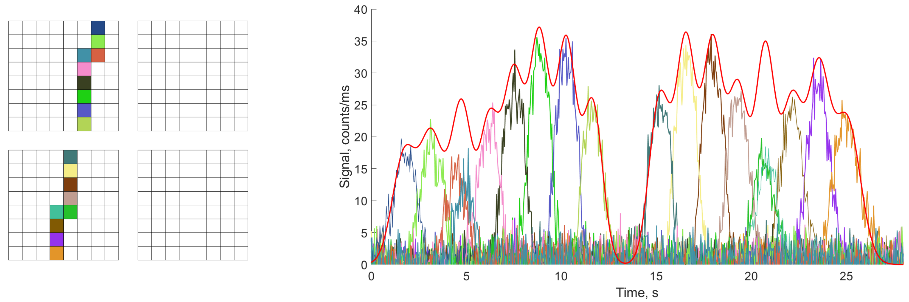
The slowest object for observation (apart from the stars), producing a straight track on the photodetector, is the orbital motion of satellites. An example of such an event is shown in Figure 5, which shows the location of triggered channels (i.e., channels in which the signal significantly exceeds the background) on the left and their signals on the right. (Colors of pixels on the channel map and signal curves match each other.) Here the signals are expressed in counts per ms.

This event corresponds to the passage of the micro-satellite BUGSAT-1 near the zenith on 8 December 2021 at 03:56:31 UTC.

To estimate the speed of the satellite, the triggered channels were divided into two groups of nine channels each before the image entered the dead zone between two PMTs and after. Reconstruction by the LTA method for the first group gave an estimate of $\mathsf{\Omega }=12.6$ mrad/s, and for the second–$\mathsf{\Omega }=12.7$ mrad/s. The speed of BUGSAT-1 was calculated on the basis of orbital parameters encoded in the two lines element (TLE) file at that moment was 12.4 mrad/s. For other events of this type, reconstruction errors can reach 10%.

The presence of a systematic error in the speed reconstruction of the track events indicates the need for both more accurate detector calibration and the use of more advanced reconstruction algorithms. In particular, the value of the LTA control parameters was chosen based on simple model events and did not take into account many features of a real detector. Well-tracked—and known to have high accuracy—the orbital motion of satellites and the movement of stars in the sky will allow us to refine these parameters and test and optimize new reconstruction algorithms.

An example of a much faster event—a meteor—is shown in Figure 6. The signal was reliably registered in 11 channels lying on the edge of one of the PMTs. As part of the light fell into the dead zone of the photodetector, the measured light curve (the red line on the right panel, it is shown with a factor of 0.5 for ease of perception) can differ significantly from the real one. Despite the fact that the time resolution of 41 ms is insufficient for a detailed analysis of meteor’s light curve, a rough estimate of the angular velocity of this event can be made: $\mathsf{\Omega }=0.25$ rad/s. This means that at a meteor altitude $H=100$ km, its apparent speed was 25 km/s.

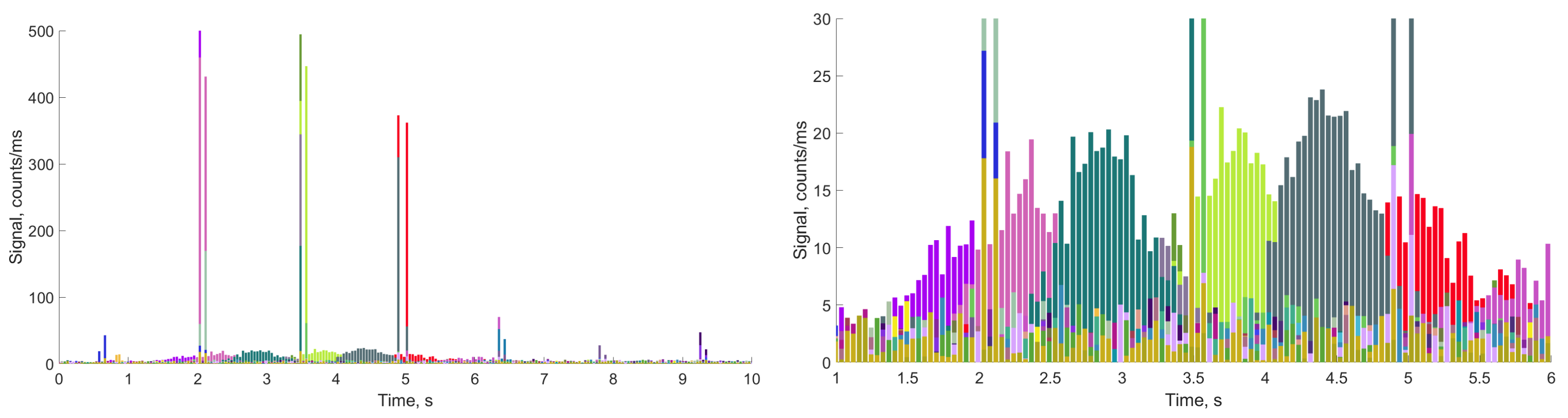
The signals of the last example of track events presented in Figure 7 look somewhat strange: along with the shifts of maxima typical for track events (see on the right), a powerful double flash occurs at a regular interval of $\sim 1.5$ s. The event was identified as a civil aviation aircraft flying on the Moscow–Murmansk route. The peaks in the registered signals correspond to the onboard flash signals of the aircraft.

The final part of the flight passes over the VTL, when the aircraft reduces its speed and flight altitude to approximately $V=550$ km/h and $H=3$ km, respectively. The angular velocity of the aircraft’s movement visible from the VTL also depends on the direction of movement and the angle of observation, but due to the relatively small FOV of the detector, in the first approximation, they can be neglected, $\mathsf{\Omega }=V/H\approx 51$ mrad/s. It is difficult to estimate the velocity using the LTA method since the event only touches the FOV along its very edge and a significant part of the radiation enters the detector as a result of scattering (presumably by clouds).

3.3. Aurora Measurements

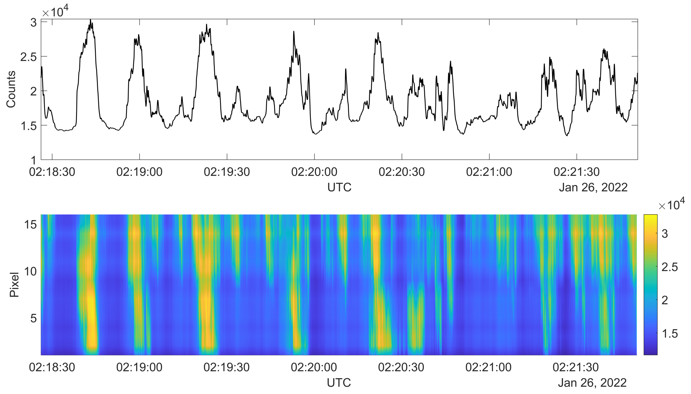
The detector works in a continuous monitoring measurement mode with a 41 ms temporal resolution, and it allows us to obtain detailed information for the whole night. In Figure 8, the example of such measurements (integral light curve of the photometer) is shown. Different temporal structures, which correspond to various types of aurora, can be seen. Intensive spikes in emissions correspond to bright aurora arcs that appear and move in the photometer FOV. After 02:00, a fast variation in emissions is seen. This is an example of PsA. The more detailed waveform and a North–South keogram (diagonal pixels of the photometer matrix that lay close to the North–South direction) are shown in Figure 9. The intensity of the pulsations, as well as their period, change with time. The so-called internal modulation with higher frequency can be recognized during the “ON’’ phase of pulsations. This type of aurora usually occurs after midnight and are observed for 1–2 h.

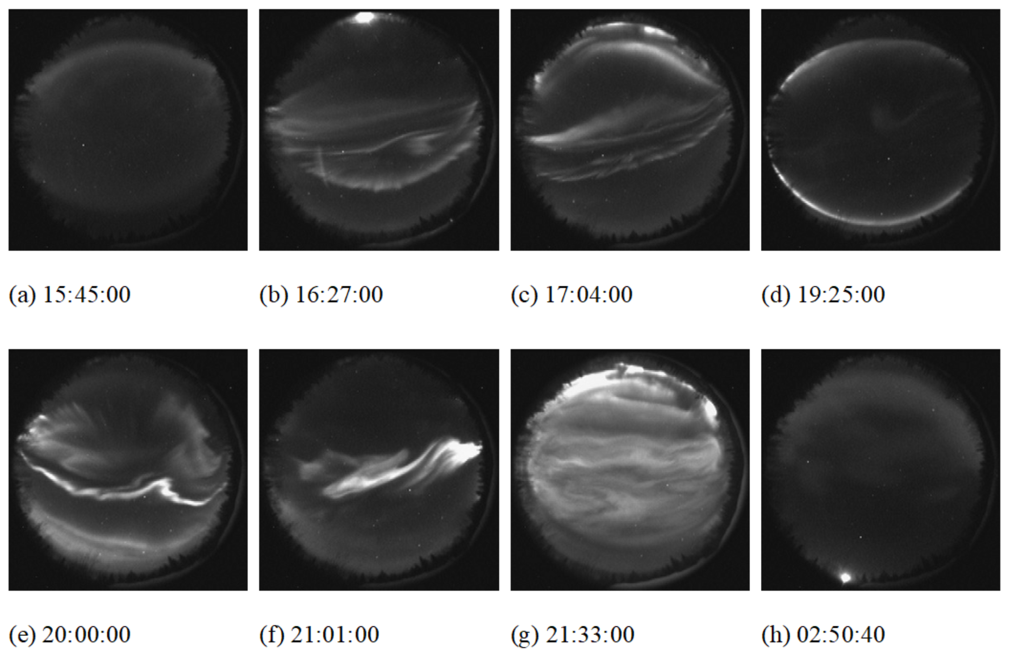
The geophysical situation during the night of 25–26 January 2022 was moderately disturbed. According to ground-based magnetic and optical data, several substorm activations were recorded on the Kola Peninsula before midnight; the SYM-H index was ∼40 nT. The auroras on the VTL all-sky camera became visible after 15:00 UT. By 15:45, the southern edge of diffuse auroras shifted to the southern horizon (Figure 10a), and an arc of the discrete aurora descended closer to the zenith from the north. Within the region between these boundaries, weak rayed forms moved from east to west. After 16:00, the auroras became more active, and a system of multiple arcs appeared (see Figure 10b). At 16:30, the movement of the entire system of arcs changed from the southward to northward direction (Figure 10c), and by 17:00, the aurora zone expanded over the entire FOV. These are the consequences of the strong substorm (AE∼1000 nT) that occurred to the east from VTL.

At 19:25, bright auroral forms came from the southern horizon (Figure 10d,e), and the AE index stayed at about 200 nT for 2 h. After 21:00 (Figure 10f), a new activation began in the west, and now the aurora movement changed its direction from predominantly western to eastern (the Harang discontinuity was crossed around 20:50). At 21:30, the aurora fills the whole sky (Figure 10g), AE = 300. Around 22:00 UT, there was a maximum in the local magnetic disturbance ($dH=150$ nT) in Lovozero. After that, the sky is filled with pulsating auroras, the brightness of which gradually fades and they shift to the north.

From 00:00 to 01:00, the activity at latitudes below 70${}^{\circ }$ N is minimal, AE $<50$ nT, SYM-H∼20 nT. However, according to the Svalbard all-sky camera data (not shown here), auroral activity in the form of active radiant arcs remained significant at latitudes south of 78${}^{\circ }$ N. After 01:40, AE increased to 150 nT, and a bright N–S arc was observed around 01:50 UT, which may be a sign of plasma injection from the far regions of the plasma sheet of the magnetospheric tail towards the Earth [37].

At this time, a strip of pulsating aurora is observed in the VTL in the north. The shift of the strip to the south was accompanied by the development of a small, up to 100 nT, negative variation (“bay”) in the H-component of the magnetic field at the Loparskaya and Lovozero observatories, as well as the appearance of noise at frequencies below 0.7 Hz, according to the data of induction magnetometers in LOZ and VTL. The glow registered at this time can be classified as a streaming pulsating aurora, in which the emerging spots quickly move from the place of appearance and disappear (Figure 10h). The spawn locations and displacement direction look chaotic. At the same time, the photometer shows intense pulsations with a higher frequency (see Figure 8). According to preliminary estimates, there are no constant dominant periods in the intensity pulsations in the range from tenths to tens of Hz, but higher fluctuations appear in the whole spectral band at frequencies above 1 Hz.

Another example of an interesting event measured on 12 October 2021 is shown in Figure 11. The significant drop in the brightness below the background level just after a high intensity can be seen for a number of peaks. It is a sequence of so-called “over-darkening” aurorae pulses. Such kinds of events have been observed previously ([38,39]), but the generation mechanism of such an over-darkening PsA is still unclarified.

4. Conclusions

The interest in observations of pulsating auroras is due to the fact that new information on the spatio-temporal structure and spectral composition of radiation can shed light on the still insufficiently studied mechanisms for the formation of high-energy particle fluxes that affect the atmosphere of the Arctic regions. This paper presents a system of highly sensitive detectors for use in stereoscopic observations. Such a setup will make it possible to observe the depth of penetration of the high-energy part of charged particles due to a relatively weak minimum and to evaluate the efficiency of acceleration mechanisms and the maximum energies of particles in the region of pulsating auroras for the first time.

The use of two prototypes of the orbital UHECR telescope, which is being developed at the SINP MSU, will make it possible to measure and reconstruct parameters of the pulsation with high temporal resolution and high sensitivity. The use of all-sky cameras and other equipment traditional for auroral research in the PGI observatories will make it possible to fit these data into the general geophysical environment to identify the current state of the near-Earth plasma.

On the other hand, the operation of the telescopes will allow additional testing of scientific equipment, development and testing of online triggers and intelligent algorithms for selecting and reconstructing events. Such tests should be carried out taking into account the “non-ideal” optics of the devices (blurring of the image) and the inhomogeneity of the distribution of sensitivity along the channels of the photodetector. Testing of the proposed algorithms will be carried out on real (not model) events with a simple space-time pattern.