Abstract
The Global Precipitation Measurement Dual-Frequency Precipitation Radar (GPM-DPR) provides an opportunity to investigate hydrometeor properties. Here, an evaluation of the microphysical framework used within the GPM-DPR retrieval was undertaken using ground-based disdrometer measurements in both rain and snow with an emphasis on the evaluation of snowfall retrieval. Disdrometer measurements of rain show support for the two separate prescribed relations within the GPM-DPR algorithm between the precipitation rate (R) and the mass weighted mean diameter () with a mean absolute percent error () on R of and and a mean bias percentage () of and for the stratiform and convective relation, respectively. Ground-based disdrometer measurements of snow show higher MAPE and MBP values in the retrieval of R, at and , respectively, compared to the stratiform rain relation. An investigation using the disdrometer-measured fall velocity and mass in the calculation of R and illustrates that the variability found in hydrometeor mass causes a poor correlation between R and in snowfall. The results presented here suggest that retrieval is likely not optimal in snowfall, and other retrieval techniques for R should be explored.
1. Introduction
Global retrievals of precipitation that falls as rain and snow at the surface and aloft are important for quantifying several key components of the Earth’s water cycle. At the surface, the amount of snow that falls within a watershed located in mountainous terrain is vital for water supply and water resource management [1]. Furthermore, even though most of the Earth’s precipitation reaches the surface as rain, more than 60% of precipitation on average can be connected to ice phase processes aloft [2]. Thus, in order to obtain a complete quantitative understanding of the hydrologic cycle, an accurate retrieval of snowfall is required. Moreover, quantifying the total amount of ice mass in the atmospheric column (i.e., the ice water path (IWP)) has direct implications on the Earth’s radiative balance and is important for constraining general circulation models [3,4].
One method of retrieving snowfall properties is the use of radar. Since the first use of radar in atmospheric sciences, studies have shown that snowfall mass—and thus the precipitation rate—is related to the power scattered back to the radar [5]. In this work, the abbreviation R is used for the precipitation rate and is used to refer both to the rainfall and snowfall rate. Current spaceborne radars, such as CloudSat [6] or the Global Precipitation Measurement mission’s Dual-Frequency Precipitation Radar (GPM-DPR [7]), attempt to retrieve snowfall properties such as R, ice water content (IWC), and in the case of GPM enabled by its dual frequency measurements, the mass-weighted mean diameter () and characterize the spatial distribution of precipitation rate and microphysical properties.
As the first spaceborne radar designed to observe clouds and precipitation at high latitudes, CloudSat has been used to retrieve global distributions of near-surface retrieved snowfall. In [8,9], the authors were the first to investigate global retrievals of snowfall which contained large uncertainty (e.g., a factor of 10; see figure 1 in [10]) since the basis of the retrieval required the use of a power-law relation between the measured equivalent radar reflectivity factor () and the corresponding snowfall rate (also known as a relation), which is sensitive to the assumed particle type used in its formulation. In order to reduce uncertainty, renewed investigations of the global distribution of snowfall [11,12,13,14] use the CloudSat 2C-SNOWPROFILE product, which uses an optimal estimation technique [15] to retrieve snowfall rate and produce an uncertainty estimate [16,17]. Since the release of the 2C-SNOWPROFILE, studies have compared the CloudSat retrieval of R to ground-based techniques and show encouraging results [18,19,20,21], enhancing confidence in the use of the CloudSat 2C-SNOWPROFILE to retrieve global snowfall properties.
In an effort to expand NASA’s earth observing capabilities with an emphasis on global precipitation, GPM-DPR was launched into orbit in early February 2014. With the new spaceborne radar, new retrievals of global rainfall and snowfall properties could be obtained (e.g., [22,23]). Since GPM-DPR is a scanning Ku and Ka-band radar, while CloudSat is a non-scanninng W-band radar, it requires its own suite of retrievals that make a range of different assumptions. Once a sufficient sample size of near-coincidences between satellites was obtained, the authors in [24] investigated GPM-DPR’s ability to detect snowfall events using CloudSat as a reference. They found that GPM-DPR does not detect more than 90% of the detected snowfall events by CloudSat, attributing this to GPM-DPR’s lack of sensitivity. Furthermore, in [24], the authors showed that GPM-DPR’s retrievals of R in falling snow have a large low bias. The bulk statistical evaluation of the GPM-DPR and CloudSat retrieved products in falling snow by the authors in [14] showed that the global average retrieved GPM-DPR near-surface snowfall rate is about 43% lower compared to CloudSat even after carefully considering the differences in sampling (e.g., footprint size), sensitivity and operating frequency. Regional differences show much larger disparity (see Figure 7 in [14]). The low bias in the GPM-DPR snowfall retrieval is also shown by [25], where the GPM-DPR’s snowfall retrieval was considerably lower than relationships derived from measurements collected during the Olympic Mountains Experiment (OLYMPEX [26]), the Global Precipitation Measurement Cold Season Experiment (GCPEX [27]) and a mass flux technique that uses mass continuity through the melting layer and more constrained retrievals in rain. Since various investigators and methods have shown consistent results, it is evident that the current GPM-DPR retrieval in snowfall is consistently biased towards low values of R. Furthermore, the results in [14] suggest that the likely reason for this low bias is the GPM-DPR retrieval algorithm itself and not the satellite hardware (e.g., calibration, sensitivity, footprint size, scanning/non-scanning) or orbit (e.g., inclination, sun synchronous/non-sun synchronous).
A primary microphysical assumption made within the GPM-DPR retrieval algorithm is that there is a prescribed empirical relationship between R and . The relation used is derived ultimately from ground-based disdrometer measurements in the Tropics [28,29] and allows the simultaneous retrieval of R and for a measured . This framework was first adopted in version 4 of the GPM-DPR algorithm (released in 2016) and is used currently (version 6) for all precipitating echoes regardless of hydrometeor phase.
Evaluations of GPM-DPR retrieval products within rain have been ongoing. Studies have considered the direct evaluation of GPM-DPR retrievals with surface-based rain gauges [30], radars [31] and disdrometers [32]. Results generally show a good agreement and meet the Level 1 Scientific Requirements of the GPM mission (see Section 1.1.3 of [33]). However, there have been no investigations of the empirical relation itself and whether it can encapsulate observations of rainfall from various meteorological regimes. Furthermore, no studies have verified that the same empirical relation applies to snowfall.
The analysis provided here will assess the empirical relation prescribed between R and using surface observations of rainfall from various geographic locations and will quantify its error. Then, observations of surface snowfall will be contextualized in the liquid equivalent space for a direct evaluation of the relations used in the GPM-DPR retrieval algorithm. The structure of the rest of the manuscript is as follows: Section 2 describes the datasets used in this study and how the data were collected and discusses how PSD parameters are derived from both liquid and solid-phase PSDs. Section 3 presents the results of how well relations generated using PSDs measured in both rain and snow compare to the prescribed relation in the GPM-DPR algorithm, quantifies error in retrievals emulating the GPM-DPR algorithm and investigates the correlation between R and . Section 4 presents a brief summary and states the overall conclusions and some future research ideas.
2. Data and Methodology
2.1. Measurements
2.1.1. Rainfall Data
In order to evaluate the applicability of the prescribed relationships within the GPM-DPR algorithm in rain, data collected as part of NASA Ground Validation (GV) field campaigns and Department of Energy-Atmospheric Radiation Measurement (DOE-ARM) mobile facility deployments are used. The NASA GV field campaigns have accumulated numerous surface-based rainfall PSDs over numerous geographic locations around the United States of America. Specifically, the campaign data used here are from the following projects: Mid-Latitude Continental Convective Clouds Experiment (MC3E, Oklahoma [34]), the Iowa Flood Studies (IFloodS, Iowa), Integrated Precipitation and Hydrology Experiment (IPHEx, North Carolina [35]), and the Olympic Mountain Experiment (OLYMPEX, Washington State [26]). Data collected at two sites that were not a part of official campaigns but nevertheless are included in the NASA GV database are also used here, namely data collected in Huntsville, Alabama and at Wallops Air Force Base, Virginia. In order to add samples from outside the United States, data are included form several DOE-ARM campaigns and fixed field sites of DOE-ARM. Specifically, data from the following international sites are used: Cloud, Aerosol and Complex Terrain Interactions (CACTI, Cordoba, Argentina [36]), Tropical West Pacific (TWP, Darwin, Australia and Manus Island, Papua New Guinea [37]), Dynamics of the Madden-Julian Oscillation/ Cooperative Indian Ocean experiment (DYNAMO/CINDY2011, Gan Island, Maldives [38]) and Eastern North Atlantic (ENA, Graciosa Island in the Azores, Portugal [39]). Finally, a long-term record from the Southern Great Plains (SGP) site at Lamont, Oklahoma is used [40].
For all the aforementioned campaigns and field sites, data from a two-dimensional video disdrometer (2DVD [41]) are used. The 2DVD is commonly used as a reference disdrometer (e.g., [42,43,44]) that measures particle maximum dimension, shape and fall velocity. The minimum particle size that can be sampled reliably by the 2DVD is 0.2 mm [41]. The specific data used here are the processed datafiles that remove particles that have a terminal fall velocity less than of the predicted fall velocity based on size following the relation in [45]. This prevents data from being contaminated by secondary drops (i.e., two drops in the sample volume at the same time). Furthermore, only time periods where the rain rate is greater than 0.01 mm hr and had more than 10 drops within 1 min were considered in the analysis. Then, measured particle size distributions (PSDs) are scaled from the 1 min averages to 5 min averages. The result of the amalgamation of all the 2DVD measurements is approximately years of raining PSDs. Overview statistics from all 2DVD data and their respective campaigns are found in Table 1.

Table 1.
Statistics of disdrometer measurements. The equations to calculate the parameters below are found in the following section, and their means (when R ≥ 0.01 mm hr) are reported in the table. The number of samples refers to the number of 5 min particle size distributions (PSDs). The means of and were calculated in linear units and then converted to the logarithmic units shown. The underlined text in the first column denotes the data source and probe.
2.1.2. Snowfall Data
From January until April 2014, a joint field campaign between NASA, the University of Helsinki, DOE-ARM and the Finnish Meteorological Institute was conducted with an intensive observation period designed explicitly to study snowfall [46]. The campaign, named the Biogenic Aerosols—Effectson Clouds and Climate experiment (BAECC), collected data with several radars (C-band, X-band, Ka-band and W-band; dual-polarized and Doppler; scanning and non-scanning), surface-based meteorological instruments, vertically pointing microwave radiometers and surfaced-based automated measurements of snowfall and its PSD. Snowfall rate was measured directly through two OTT Hydromet Pluvio2 weighing bucket gauges enclosed in a Double Fence Intercomparison Reference (DFIR) and a Precipitation Imaging Package (PIP)—the successor to the Snowflake Video Imager [47] and not to be confused with the commonly used aircraft probe, the Precipitation Imaging Probe.
The PIP is a high-speed camera pointed at a light source that is 2 m away. This allows for any particle falling within its field of view (48 mm × 64 mm) and between the light source and the camera to cast a shadow. From these videos of shadowed particles, the particle size and fall velocity can be diagnosed. Since the terminal fall velocity is explicitly measured for each particle, the derivation of the mass of each particle can be deduced if atmospheric base state information (i.e., pressure, temperature) is known. Effectively, the mass can be estimated through hydrodynamic theory by considering the drag on the particle, the buoyancy of the particle in the fluid (i.e., air) and gravity [48,49]. This method has been used on other ground-based disdrometers [50,51,52,53] as well as the dataset used herein [54,55,56]. For a more complete discussion of the retrieval of the mass and its intricacies, consult Section 3a from [54]. After the BAECC campaign concluded its snowfall IOP, the PIP and weighting bucket gauges remained at the measurement site in southern Finland and are currently still collecting observations. Thus, the ongoing record is now five complete winter seasons. Since the processing of the PIP data and retrieval of mass is not trivial, at the time of writing this manuscript, only the data from February 2014–March 2015 were available. Summary statistics of the PIP data are shown in Table 1 for comparison against the 2DVD datasets.
2.1.3. Data Availability
All rainfall data are free for use can be found in two main locations, the NASA GHRC [57] and ARM DOE data discovery [58]. The processed snowfall observations, including the retrieved mass, can be found on github [59]. For convenience, some data and the current version of the Algorithm Theoretical Basis Document (at the time of submission) is found on the github site [60].
2.2. Particle Size Distribution Parameters
2.2.1. Rainfall PSD Parameters
The precipitation rate for rain can be determined from a measured PSD by
where is the volume of liquid water, is the terminal fall velocity and is the number distribution function for particles with a maximum dimension of , where is the bin width and the subscript i indicates the bin of the measured PSD. The characteristic size of mass weighted mean diameter () can also be determined from a measured PSD as
where is the mass of the particle with a maximum dimension of . The bounds of the summation for Equations (1) and (2) are the minimum () and maximum () trusted size bin of the 2DVD, which are 0.2 mm and 10 mm, respectively. If the raindrops are assumed to be spherical, then the volume and mass of a raindrop with size can be substituted into Equations (1) and (2) as follows:
In reality, raindrops larger than 1 mm are not observed to be spherical [61]. On average, if R and are calculated from the PSDs using a sphere versus a spheroid with the axis ratio predicted in [62], there is approximately a and overestimation of R and , respectively (not shown). While this is not a trivial amount of error, it is a noted limitation of the work, and assessing the raindrop shape assumption within GPM-DPR is a topic of future research.
Under the Rayleigh assumption (generally applicable in S and C-band weather radar retrievals) where the wavelength of the radar is much greater than the maximum dimension of the particle, the equivalent radar reflectivity factor () is given by
Since the GPM-DPR consists of Ku and Ka-band radars, there could be instances in which Rayleigh scattering is not a valid assumption. To avoid additional inaccuracies on the wavelength dependence, the Ku and Ka-band are calculated as
where is the radar frequency, is the dielectric constant (0.93) and is the backscatter cross-section of a spherical raindrop of maximum dimension . The is determined using T-matrix theory [63] as implemented by the pytmatrix python package ([64] https://github.com/jleinonen/pytmatrix). As noted previously, the spherical assumption may not always be correct, and assuming a sphere results in an average overestimation of by approximately .
In order to classify PSD points into convective or stratiform (Section 3.1), additional PSD parameters are required. One of the additional parameters is the normalized intercept parameter (), which is defined as
where is the density of liquid water and is the liquid water content, defined as
The last PSD parameter needed is known as the median volume diameter (), which, when assuming the presence of a gamma size distribution shape, can be written as
where is the shape parameter of the three-parameter gamma distribution. The relation from [65] between the standard deviation of the mass distribution () and is used to define by
where is defined as
2.2.2. Snowfall PSD Parameters
The conversion from a solid precipitation rate to liquid equivalent snowfall rate is straightforward and not novel to this study. Equation (1) is re-written with and , where represents the retrieved mass estimate of a particle with from the PIP,
Calculating a liquid equivalent is not as direct and not commonly done in the literature. The liquid equivalent diameter () needs to be considered in Equation (2), which—if a sphere is assumed as the melted shape—can be determined by
Then, Equation (2) becomes
The conversion of and to a melted equivalent (e.g., ) is not done for the following reason. Consider Figure 1, where two sample volumes are depicted: one with frozen hydrometeors and the other with the liquid equivalent. If it is assumed that all particles within some bin are of the same particle type and that the melted version of the particle forms a sphere (i.e., no breakup), then the particles simply translate to smaller, higher density versions of themselves. This then preserves the original number of particles, and thus the product of is equivalent to , and the integrated parameters such as and total number concentration are preserved.
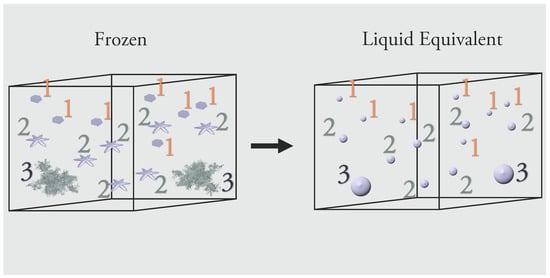
Figure 1.
Schematic diagram to illustrate the conversion of the measured solid phase size distribution of particles to the liquid equivalent. The box is an instantaneous sample volume, and the particle diagrams are from ARTS ([70] https://zenodo.org/record/1175573). Each number corresponds to the same bin.
In reality, all particles found in one size bin are probably not the same particle type (e.g., same habit, same degree of riming). To account for this, separate PSDs for different habits would need to be known. Since the variability of habits and particle densities within each size bin are not well known and are difficult to determine, the assumption of a single particle type is used.
In order to calculate for snowfall, Equation (6) is used. The only change is in how is determined. To avoid the issues of underestimating the when using Mie or T-matrix theory at higher operating frequencies (Ka-, W- band [66]), is derived following the technique in [67]. The authors of that work simulated several different degrees of rimed aggregates, and their corresponding scattering properties were determined from the Discrete Dipole Approximation (DDA [68]). Since particles can have a variety of degrees of riming, and thus a variety of masses with the same maximum dimension, Equation (6) becomes
where is determined from the and retrieved by the PIP. This is done using the kd-tree search algorithm from Scipy [69], which efficiently searches the [67] database of particles for the particle with the most similar and . This method was chosen instead of taking the median or mean over all particles simulated in order to allow the natural variability in to propagate into the forward calculation of .
2.3. GPM-DPR Algorithm
A complete description of version 6 of the GPM-DPR algorithm can be found in the Algorithm Theoretical Basis Document (ATBD, [71]). The microphysical basis of the algorithm assumes the R and are well correlated, and thus a mathematical relation can be formulated between the two parameters. Specifically, the relations used to relate R and in the GPM-DPR algorithm are
for convective precipitation and
for stratiform precipitation. In both expressions, is a diagnosed parameter that is constant in the atmospheric column and is used to reconcile estimates of path integrated attenuation (PIA) and the retrieved PSD parameters. The default value is , but this is logarithmically varied between and 5. The relationship between , R and can be calculated with some assumptions about the PSD. In the GPM-DPR algorithm, the form of the PSD is assumed to be the normalized three-parameter (;;) gamma distribution [72]:
The parameter in the GPM-DPR algorithm is assumed to be three; thus, the PSD can be described using two parameters: and . Equation (1) can then be rewritten with the GPM-DPR assumptions in integral form as
where in the GPM-DPR algorithm follows [73]
.
Similarly, Equation (6) can be rewritten as
where particles are assumed to be spherical and Mie theory is used to determine . Since the relation between R and is prescribed (Equations (16) and (17)), Equation (19) can be algebraically manipulated to solve for
Then, all parameters needed to calculate for each R and pair are known. In order to solve the integration of the indefinite integrals (Equations (21) and (22)), quadrature is used. Specifically, the Scipy [69] quadrature is used, which uses the FORTRAN QUADPACK [74] to perform automatic integration. The result of solving for is shown in Figure 2, assuming particles are in the liquid phase. Furthermore, the result of varying within the relation is shown in Figure 2b. Effectively, as expected, the value increases away from the origin (i.e., larger characteristic sizes and larger precipitation rates).
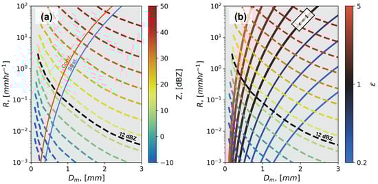
Figure 2.
Precipitation rate (R) and mass weighted mean diameter () theoretical diagrams. (a) The default () relation for both convective (solid red line) and stratiform (solid blue line) regimes with the equivalent radar reflectivity factor () in logarithmic units (dBZ) is contoured (dashed rainbow lines) assuming rain. The contours are determined using the same assumptions as those in the GPM-DPR algorithm for a range of values. The dashed black line is the 12 dBZ, contour which is the GPM-DPR Ku-band minimum sensitivity. (b) Similar to (a), the rainbow contours are the , while the other lines are the stratiform relation, but now the parameter is varied. The default relation () is in black, while is in red shades and is in blue shades.
The retrieval process can be found in the ATBD [71] but is described here briefly. Assuming that GPM-DPR has an observed profile containing precipitation echoes, the algorithm diagnoses whether the profile of is convective or stratiform based on the vertical structure of . This is most simply done by considering if a melting layer can be detected in (i.e., radar bright-band). Additional methods are used and can be found in Section 3.5 in the ATBD [71]. Then, the phase of each radar gate is assigned using temperature information from numerical weather prediction and the location of the radar bright-band if present. Radar gates found 500 m above the radar bright-band or at temperatures less than 0 C are designated as solid phase. The solid phase designation assumes that the particles contained within the gate are solid spherical particles with an effective density of 0.1 g cm. Radar gates found below 500 m of the radar bright-band or temperatures greater than 0 C are designated as liquid phase (i.e., spherical with effective densities of 1 g cm). After the phase is determined, the observed and the initial estimate of () are used to search for where the relation intersects the contoured , thus simultaneously retrieving R and . Once R and are retrieved for all radar gates with precipitation echoes, the PIA and Ka-band can be calculated. This process is repeated with different values of , and the optimal value of is chosen by minimizing the difference of the retrieved PIA with the estimated PIA and the retrieved Ka-band with the measured Ka-band if available. If only Ku-band is measured, then only the PIA error is used in the optimization. For a more complete description of the algorithm, consult the ATBD.
It should be emphasized that an relation derived from surface rain observations is used for the entire atmospheric column, regardless of whether the gates are identified to contain ice or snow. The only differences between the solid phase retrieval and the liquid phase retrieval is the complex index of refraction needed for the determination of , the and a slightly modified version of Equation (18) (ATBD page 68). To the authors’ knowledge, the effect of using the rain relation on snow has not been investigated. It is hypothesized here that the use of a rainfall relation in snowfall retrieval could potentially account for the large low bias reported in [14].
3. Results and Discussion
3.1. Rainfall
The GPM-DPR algorithm documentation is not explicit regarding the origin of the relation, but it can be found in [28]. In that work, it was noted that the relations were derived using the methodology in [29] on a limited disdrometer dataset that would be tested on more PSD observations in future work. It is noted that the data used in [29] are derived from an impact disdrometer described in [75], which has been shown to potentially undercount small and large drops relative to the 2DVD [76]. In order to assist in these efforts, an investigation of the relationship in rainfall is conducted here. The 2DVD dataset provides an opportunity to evaluate whether the relation used in the GPM-DPR algorithm is general enough to apply to PSDs applicable to global precipitation measurements. All PSD data from the 2DVDs measured in rain are considered in a bulk sense in Figure 3, without separation into convective or stratiform regimes. The 2D histogram of the density of observations (Figure 3a) shows that the majority of points follow the general shape of the relations and lie between the convective–stratiform curves for (Figure 3a, red and blue curves). The mode of all the observations (Figure 3b), also lies between the convective–stratiform relations, with it being centered on the stratiform curve for 1.5 mm and centered on the convective curve for 1.5 mm. This is consistent with expectation that convective rainfall generally produces larger R and larger . The relationship with Ku-band is shown in Figure 3c, where increases with increasing R and . Overall, the 2DVD observations collected around the world support the use of the relation in retrievals of rainfall and are consistent with the current framework used within the GPM-DPR algorithm. Since the Ku-band is calculated for each raining PSD, the retrieval of PSD parameters using the GPM-DPR microphysical assumptions (Section 2.3) can be emulated as if they were observed radar reflectivity values. This is done by using the relations illustrated in Figure 2a (). Then, for each raining PSD, the calculated can be used to retrieve R and . Using these retrieved R and values, error metrics can be derived by comparing the retrieved values to the calculated values from the PSD. Specifically, the mean absolute error (), mean absolute percent error (), mean bias percentage () and root mean squared error () are used, which are formulated as follows:
and
where is the retrieved value and is the calculated value. The calculation of the aforementioned error metrics for the entire 2DVD dataset is found in Table 2. Without the classification of the PSDs (i.e., convective or stratiform), the error is 40–50% and 20–30% for R and , respectively.
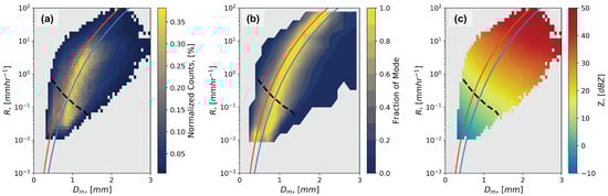
Figure 3.
Investigating the relationship between R and from all the ground-based 2DVD disdrometers in rain. (a) Counts of observations on the plane normalized by the total number of observations and converted to percentages. Only bins with at least 10 observations are shown. The same relations of and the minimum sensitivity from Figure 2a are shown for reference. (b) Same data as (a), but the data are normalized to the total number of observations in each bin of R. A value near one implies that it is near the mode of observations in that bin of R. (c) Same 2D histogram as (a), but colored by the bin median value of Ku-band calculated from the PSD assuming spheres and using a Tmatrix.
Table 2.
Error statistics for the entire 2DVD dataset. MAE: mean absolute error; MAPE: mean absolute percentage error; MBP: mean bias percentage; RMSE: root mean square error.
From Figure 3, it is not immediately apparent that there should be two distinct relations. To assess if two relations should be used, a convective–stratiform partitioning of the data could be used. Since thermodynamic profiles are unavailable for all raining instances in the database and reanalysis would likely struggle to diagnose the observed buoyancy on the spatial and temporal scale needed to diagnose convection, there is no way to categorize the data based on thermodynamic variables, and coincident radar data are not available to perform a radar-based separation [77]. Thus, the only viable way to categorize the data into convective and stratiform regimes is to use relationships derived from the PSD parameters themselves, such as the relationship between and , as used in [78,79,80]. In [79], the authors showed that PSDs with a greater than that given by the expression
were diagnosed as convectively produced, while PSDs with less than Equation (27) were produced by stratiform vertical motions. In [80], the authors continued this work and added an additional constraint for weak convective instances, stating that corresponds to convective and to stratiform regions; however, the work presented in [78] noted that a convective–stratiform separation based solely on may only apply in warm-rain-dominated convection over tropical oceans. In [78], the authors used Empirical Orthogonal Functions (EOF) to diagnose stratiform and convective rain and created polygons enclosing the relevant regions on the plane. Here, the polygons in that work are used to determine the classification (Figure 4a). The result of separating the observations shown in Figure 3 into stratiform and convective categories is shown in Figure 4. The observations show a clear separation, with the convective-labeled points closer to the convective relation, while the stratiform-labeled points are indeed closer to the stratiform relation (Figure 4b). Similarly, the convective and stratiform relations lie close to the mode of their respective classified points (Figure 4c). The same error metrics from Table 2 are recalculated for the category-specific data and shown in Table 3. All metrics improve by sub-setting the data, except for the convective rainfall rate retrieval. This is likely a result of most of the points being located at a smaller R than the relation, centered around = 1.2 mm for the convective labeling. However, the is similar, at and for the “not classified” and “classified” data, respectively.
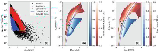
Figure 4.
Convective–stratiform partitioning based on PSD parameters. (a) Normalized intercept parameter () median volume diameter () plane of all raining PSDs. The red points are labeled as convective and blue are labeled as stratiform based on the classification in [78]. The polygons from [78] are drawn in solid blue (stratiform) and dashed red (convective). (b) Same as Figure 3a, but with the separated categories. Red is convective, blue is stratiform. The lighter the color, the higher the density of points. (c) Same as Figure 3b, but with the separated categories. Colors are the same as (b).
Table 3.
Error metrics for the 2DVD data after classifying the PSD data based on the values of , and [78].
3.2. Snowfall
In this section, the entirety of the snowfall PSDs observed in Finland are analyzed in the same bulk way that was done for the rainfall results presented above. Figure 5 shows the results of calculating the liquid equivalent R and liquid equivalent from the snowfall PSDs. The highest density of observations is found at a smaller and larger R than prescribed by the relation with (Figure 5a). Furthermore, the ranges of both R and in snow (Figure 5) are less than that of rainfall (Figure 3). The mode of the snowfall distribution is closest to the stratiform curve for 0.5 mm 0.75 mm but then deviates from both empirical relations at a larger (Figure 5b). The calculated Ku-band (Figure 5c) increases with increasing R and , similar to the rainfall data analysis shown above. The snowfall PSD observations from Finland suggest that the relationship with does not fit well and could be a large source of error in the algorithm.
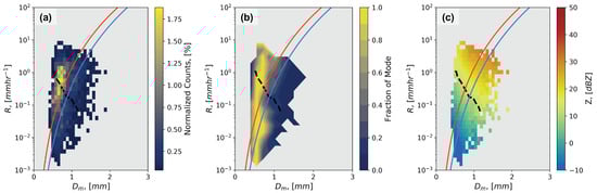
Figure 5.
As in Figure 3, but now for the snowfall PSDs collected in Finland. The x and y axis are in their liquid equivalent values (see Section 2.2.2) (a) Counts of observations on the R − plane normalized by the total number of observations and converted to percentages. The same relations of R − Figure 2a are shown for reference. (b) Same data as (a), but the data are normalized to the total number of observations in each bin of R. A value near one implies that it is near the mode of observations in that bin of R. (c) Same 2D histogram as (a), but colored by the bin median value of Ku-band calculated from the PSD using the method described in Section 2.2.2.
In order to quantify error in the same manner as before, the GPM-DPR algorithm is emulated, but now using the solid phase assumptions. The retrieval metrics are shown in Table 4. There are errors of and for the retrieval of R using the stratiform and convective relation, respectively. This is a increase in error when compared to the stratiform relation and stratiform-classified PSDs in rain. The error for the retrieval of is not as large as the retrieval of R, at and for the stratiform and the convective relation, respectively.
Table 4.
Error metrics from the snowfall data measured in Finland.
One potential way to improve retrievals could be to fit new coefficients to Equations (16) and (17), but the snowfall PSD data suggest that an framework may not be advantageous for retrievals in snowfall because of the lack of correlation between and (Table 5). Snowfall PSDs have a correlation value of , which is approximately half of the correlation value derived from rain, at . The poor correlation in snow persists regardless of whether the conversion of to liquid equivalent is considered (Table 5). Thus, even fitting new coefficients to Equations (16) and (17) might not result in optimal snowfall property retrieval.
Table 5.
Pearson correlation values between and for the entire rain dataset and the snowfall measurements in Finland.
3.3. Investigation of Poor Correlation between R and in Snowfall
Two hypotheses are formulated to explain the poor correlation between R and in snow. One hypothesis is that the velocity–diameter relation and its natural variability in snow causes a reduction in the correlation between R and . The second hypothesis is that the mass–diameter relation of snow and its natural variability causes a reduction in the correlation between R and . Both hypotheses are tested by imposing velocity and mass relations derived from snowfall into the calculation of R and in rain. The goal of replacing the velocity and mass relations in this way is to test the sensitivity of the correlation of R and and whether the poor correlation in snow can be reproduced by the rain dataset. The snowfall speed and mass relations are derived from the PIP snowfall observations, where the particle’s observed maximum dimension is related to fall velocity and mass. The mean fall velocity and mass for the entire dataset is shown in Figure 6 (blue) alongside the default assumptions for the rainfall (red) and some parameterizations from previous studies (black). In order to test the first hypothesis, the fall velocity (e.g., in Equation (1)) is sampled from a normal distribution with a mean and standard deviation of that in snow; in other words, the fall velocity at any diameter is randomly sampled from the normal distribution with the mean and standard deviation determined from the data in Figure 6a. Similarly, in order to test the second hypothesis, the mass (e.g., in Equations (1) and (2)) is sampled from the mean and standard deviation of snow particle masses.
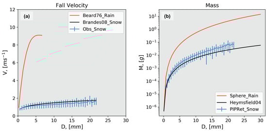
Figure 6.
Fall speed and mass diameter relations for rain and snow. (a) Particle fall velocity for rain (red) determined by the empirical relation from [45]. Mean (blue centerline) and one standard deviation (blue bars) particle fall velocity for snow measured by the PIP and the predicted fall velocity at −1 from [81] (black). (b) Particle mass for rain (red) determined by assuming a spherical shape. Particle mass for snow as retrieved from the PIP and predicted by the relation in [82].
For these tests, the following substitutions are made: replace , replace and replace both and . The results of these three experiments are shown in Figure 7, and their respective correlations are reported in Table 6. Replacing only the fall speed relation results in a 0.08 reduction in the correlation compared to the original rainfall analysis (; Figure 3a). As expected, there is a reduction in the magnitude of R since the fall velocity magnitude has been decreased and has remained the same because is not a function of (Figure 7a). Substituting the mass relation results in a much larger magnitude reduction in the correlations (), yielding similar correlation values () to those found from the snowfall data. Figure 7b shows that there is now not only a reduction in the magnitude of R but also in . Finally, replacing both relations results in the same correlation as swapping the . It should be noted that the experiments shown in Figure 7 are applied separately and randomly (i.e., through the normal distribution) despite knowing that the is not mutually exclusive from (e.g., more massive particles fall faster, absence of drag). Thus, these experiments are likely missing the co-variability between and that could improve the calculated correlation values.
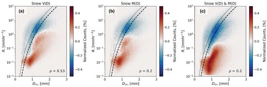
Figure 7.
Recalculating R and for rain using measured snowfall relationships. (a) Difference in the normalized counts between the new calculation of R and using the measured snowfall velocity relationship (shown in Figure 6a) and the original calculation (same as Figure 3a). (b) Same as (a), but with R and calculated with the measured snow mass relation (shown in Figure 6b).
Table 6.
Pearson correlation coefficient between and for the experiments in Figure 7.
Substituting the mean mass relation from the PIP observations above is effectively using one a and b value in the common parameterization of ice particle mass:
The effective curve fit values of a and b from all the snowfall data presented here are 0.1 g cm and , respectively, determined by the Scipy [69] curve fit method. In order to determine how the correlation varies across a wide range of possible a and b, the formulation for mass from Equation (28) is adopted, but a and b are systematically varied when inserted into Equation (1) and Equation (2). It should be noted that typical values of a and b in ice and snow are g cm g cm and , respectively [83]. The fall velocity relation used here is the same as the original rainfall analysis [45]. First, the result allowing no variability in the mass (i.e., the mass is exactly prescribed by Equation (28)) is investigated (Figure 8a) and shows that the correlation between R and is only a function of b, which can be expected, as the a parameter will cancel out in Equation (2). Note that the magnitude of the correlation for the fits a and b for the snowfall data, which is between and , is much larger than that reported in Figure 7b (). This shows that the magnitude of the mass is less important when determining the correlation of R and , while the natural variability of mass for any particle size determines the correlation between R and . To illustrate this further, the a and b values are systematically varied again, but now the natural variability in hydrometeor mass is added in a similar to that done previously by sampling a normal distribution with the mean predicted using Equation (28) and the standard deviation determined by the snowfall observations (Figure 6b). The results are shown in Figure 8b and show that, for larger a values ( g cm) a similar relationship to Figure 8a is found. But for small a values, where many empirical fits for snow and ice have been found ( g cm g cm and ; see [83] Figure 1), the correlation is low for any value of b. Thus, for a majority of ice and snow, it is likely that the correlation between R and is poor. Doing the same type of analysis on the snowfall PSDs (e.g., removing the natural variability and replacing it with the rainfall relations) resulted in improved correlations between R and to about , which is the same value achieved for rain with static a and b values (Figure 8a).
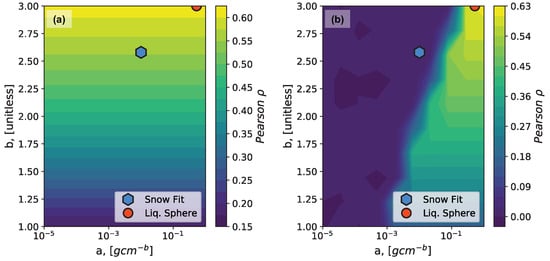
Figure 8.
Investigating the variance of the correlation between R and with various a and b values in the calculation of mass (). (a) No variability in Equation (28) is used. The hexagon is the fit a and b values to the entirety of the Finland snowfall data, while the circle is the values for a liquid sphere. (b) Same as (a), but now the mass is randomly sampled from a normal distribution with the mean predicted by Equation (28) and the standard deviation given from the observations shown in Figure 6b.
4. Conclusions
Since being launched in 2014, the Global Precipitation Measurement (GPM) Dual-Frequency Precipitation Radar (DPR) has collected copious equivalent radar reflectivity factor () measurements of both rain and snow. Microphysical parameters of interest, such as the precipitation rate (R) and mass weighted mean diameter (), are retrieved and published. An evaluation of R retrieved for snowfall by GPM-DPR reported the current status of the GPM-DPR algorithm, showing an approximately low bias on the global mean snowfall rate compared to CloudSat [14]. In order to investigate the potential causes of this low bias, the main microphysical assumption that the particle size distribution (PSD) follows an relation was evaluated. The principal conclusions are as follows:
- Assuming that raindrops are spherical, ground-based 2D-video disdrometer measurements of rainfall from various geographic locations show good agreement with the current GPM-DPR algorithm framework, with the majority of observations being found near the prescribed GPM-DPR relation and a Pearson- correlation coefficient of between and (Figure 3, Table 5).
- The classification of PSDs as convective or stratiform according to the method in [78] (e.g., based on the normalized intercept parameter () and the median volume diameter ()) is consistent with and supports the use of two separate relations for each rainfall class, as they reduce error compared with the use of a single relation (Figure 4, Table 3).
- Ground-based Precipitation Imaging Probe measurements of snowfall in Finland do not show the same consistency as the retrieval framework compared to rainfall. The error using the GPM-DPR stratiform relation is much larger ( comparing Table 3 to Table 4), and the Pearson- correlation between and is considerably lower (Pearson-; Figure 5; Table 5).
The analysis provided here suggests that the use of an relation derived in rain is inappropriate for use in snowfall. A potential alternative is to default to old techniques for deriving snowfall rate, such as the power-law fit between and R. While there can be an order of magnitude of uncertainty on single frequency relations depending on the assumed particle type [10], this is more physically based than the current GPM-DPR algorithm (version 6) in snowfall. One advantage that GPM-DPR has over its predecessors is a second operating frequency (Ka-band). Having a second frequency should allow for improved retrieval results compared to a single frequency, as shown by [84]. As a potential avenue for retrieving R and , the authors are pursuing the use of neural networks to allow for an unsupervised approach to retrieve snowfall parameters. This was done first in [85] but deserves renewed investigation since machine learning methods have improved and new multiple frequency datasets exist for retrieval implementation and evaluation (e.g., GCPEX [27]; OLYMPEX/RADEX [26]).
Author Contributions
Conceptualization, R.J.C., S.W.N. and G.M.M.; methodology, R.J.C., S.W.N. and G.M.M.; software, R.J.C.; validation, R.J.C.; formal analysis, R.J.C.; investigation, R.J.C., S.W.N. and G.M.M.; resources, R.J.C.; data curation, R.J.C.; writing—original draft preparation, R.J.C.; writing—review and editing, R.J.C., S.W.N. and G.M.M.; visualization, R.J.C.; supervision, S.W.N. and G.M.M.; project administration, S.W.N. and G.M.M.; funding acquisition, S.W.N. and G.M.M. All authors have read and agreed to the published version of the manuscript.
Funding
Funding for this research was provided to the University of Illinois by NASA Precipitation Measurement Missions grant 80NSSC19K0713 and NASA Earth System Science Fellowship 80NSSC17K0439.
Acknowledgments
The authors thank the two anonymous reviewers and the assistant editor for taking the time to review and enhance the manuscript. We also acknowledge the fruitful scientific discussions with Shinta Seto and Toshio Iguchi. Furthermore, we thank all the participants of the field campaigns used here for their tireless effort in collecting the data used in this study. Additionally, we would like to thank Patrick Gatlin for providing some of the NASA processed 2DVD data. Finally, we would like to thank Annakaisa von Lerber for her dedication and effort in providing the PIP dataset processing that was vital to the conclusions of this manuscript.
Conflicts of Interest
The authors declare no conflict of interest.
References
- Viviroli, D.; Weingartner, R.; Messerli, B. Assessing the Hydrological Significance of the World’s Mountains. Mt. Res. Dev. 2003, 23, 32–40. [Google Scholar] [CrossRef]
- Field, P.R.; Heymsfield, A.J. Importance of snow to global precipitation. Geophys. Res. Lett. 2015, 42, 9512–9520. [Google Scholar] [CrossRef]
- Waliser, D.E.; Li, J.L.F.; Woods, C.P.; Austin, R.T.; Bacmeister, J.; Chern, J.; Del Genio, A.; Jiang, J.H.; Kuang, Z.; Meng, H.; et al. Cloud ice: A climate model challenge with signs and expectations of progress. J. Geophys. Res. Atmos. 2009, 114, 1–27. [Google Scholar] [CrossRef]
- Ian Duncan, D.; Eriksson, P. An update on global atmospheric ice estimates from satellite observations and reanalyses. Atmos. Chem. Phys. 2018, 18, 11205–11219. [Google Scholar] [CrossRef]
- Langille, R.C.; Thain, R.S. Some Quantitative Measurements of Three-Centimeter Radar Echoes From Falling Snow. Can. J. Phys. 1951, 29, 482–490. [Google Scholar] [CrossRef]
- Stephens, G.L.; Vane, D.G.; Boain, R.J.; Mace, G.G.; Sassen, K.; Wang, Z.; Illingworth, A.J.; O’Connor, E.J.; Rossow, W.B.; Durden, S.L.; et al. The cloudsat mission and the A-Train: A new dimension of space-based observations of clouds and precipitation. Bull. Am. Meteorol. Soc. 2002, 83, 1771–1790. [Google Scholar] [CrossRef]
- Hou, A.Y.; Kakar, R.K.; Neeck, S.; Azarbarzin, A.A.; Kummerow, C.D.; Kojima, M.; Oki, R.; Nakamura, K.; Iguchi, T. The global precipitation measurement mission. Bull. Am. Meteorol. Soc. 2014, 95, 701–722. [Google Scholar] [CrossRef]
- Liu, G. Deriving snow cloud characteristics from CloudSat observations. J. Geophys. Res. Atmos. 2009, 114, 1–13. [Google Scholar] [CrossRef]
- Kulie, M.S.; Bennartz, R. Utilizing spaceborne radars to retrieve dry Snowfall. J. Appl. Meteorol. Climatol. 2009, 48, 2564–2580. [Google Scholar] [CrossRef]
- Hiley, M.J.; Kulie, M.S.; Bennartz, R. Uncertainty analysis for CloudSat snowfall retrievals. J. Appl. Meteorol. Climatol. 2011, 50, 399–418. [Google Scholar] [CrossRef]
- Behrangi, A.; Stephens, G.; Adler, R.F.; Huffman, G.J.; Lambrigtsen, B.; Lebsock, M. An update on the oceanic precipitation rate and its zonal distribution in light of advanced observations from space. J. Clim. 2014, 27, 3957–3965. [Google Scholar] [CrossRef]
- Kulie, M.S.; Milani, L.; Wood, N.B.; Tushaus, S.A.; Bennartz, R.; L’Ecuyer, T.S. A shallow cumuliform snowfall census using spaceborne radar. J. Hydrometeorol. 2016, 17, 1261–1279. [Google Scholar] [CrossRef]
- Kulie, M.S.; Milani, L. Seasonal variability of shallow cumuliform snowfall: A CloudSat perspective. Q. J. R. Meteorol. Soc. 2018, 144, 329–343. [Google Scholar] [CrossRef]
- Skofronick-Jackson, G.; Kulie, M.; Milani, L.; Munchak, S.J.; Wood, N.B.; Levizzani, V. Satellite estimation of falling snow: A global precipitation measurement (GPM) core observatory perspective. J. Appl. Meteorol. Climatol. 2019, 58, 1429–1448. [Google Scholar] [CrossRef]
- Rodgers, C.D. Inverse Methods for Atmospheric Sounding Theory and Practice; World Scientific Publishing Company: Singapore, 2000; Volume 2, p. 256. [Google Scholar]
- Wood, N.B. Estimation of Snow Microphysical Properties with Application to Millimiter-Wavelenght Radar Retrievals for Snowfall Rate. Ph.D. Thesis, Colorado State University, Fort Collins, CO, USA, 2011. [Google Scholar] [CrossRef]
- Wood, N.B.; L’Ecuyer, T.S.; Level 2C Snow Profile Process Description and Interface Control Document, Product Version P1_R05. NASA JPL CloudSat Project Document Revision 0.2018. Available online: http://www.cloudsat.cira.colostate.edu/sites/default/files/products/files/2C-SNOW-PROFILE{_}PDICD.P1{_}R05.rev0{_}.pdf (accessed on 10 June 2020).
- Cao, Q.; Hong, Y.; Chen, S.; Gourley, J.J.; Zhang, J.; Kirstetter, P.E. Snowfall detectability of NASA’s cloudsat: The first cross-investigation of its 2C-snow-profile product and national multi-sensor mosaic QPE (NMQ) snowfall data. Prog. Electromagn. Res. 2014, 148, 55–61. [Google Scholar] [CrossRef]
- Norin, L.; Devasthale, A.; L’Ecuyer, T.S.; Wood, N.B.; Smalley, M. Intercomparison of snowfall estimates derived from the CloudSat Cloud Profiling Radar and the ground-based weather radar network over Sweden. Atmos. Meas. Technol. 2015, 8, 5009–5021. [Google Scholar] [CrossRef]
- Chen, S.; Hong, Y.; Kulie, M.; Behrangi, A.; Stepanian, P.M.; Cao, Q.; You, Y.; Zhang, J.; Hu, J.; Zhang, X. Comparison of snowfall estimates from the NASA CloudSat Cloud Profiling Radar and NOAA/NSSL Multi-Radar Multi-Sensor System. J. Hydrol. 2016, 541, 862–872. [Google Scholar] [CrossRef]
- Souverijns, N.; Gossart, A.; Lhermitte, S.; Gorodetskaya, I.V.; Grazioli, J.; Berne, A.; Duran-Alarcon, C.; Boudevillain, B.; Genthon, C.; Scarchilli, C.; et al. Evaluation of the CloudSat surface snowfall product over Antarctica using ground-based precipitation radars. Cryosphere 2018, 12, 3775–3789. [Google Scholar] [CrossRef]
- Tang, G.; Wen, Y.; Gao, J.; Long, D.; Ma, Y.; Wan, W.; Hong, Y. Similarities and differences between three coexisting spaceborne radars in global rainfall and snowfall estimation. Water Resour. Res. 2017, 53, 3835–3853. [Google Scholar] [CrossRef]
- Adhikari, A.; Liu, C.; Kulie, M.S. Global distribution of snow precipitation features and their properties from 3 years of GPM observations. J. Clim. 2018, 31, 3731–3754. [Google Scholar] [CrossRef]
- Casella, D.; Panegrossi, G.; Sanò, P.; Marra, A.C.; Dietrich, S.; Johnson, B.T.; Kulie, M.S. Evaluation of the GPM-DPR snowfall detection capability: Comparison with CloudSat-CPR. Atmos. Res. 2017, 197, 64–75. [Google Scholar] [CrossRef]
- Heymsfield, A.; Bansemer, A.; Wood, N.B.; Liu, G.; Tanelli, S.; Sy, O.O.; Poellot, M.; Liu, C. Toward improving ice water content and snow-rate retrievals from Radars. Part II: Results from three wavelength radar-collocated in-situ measurements and CloudSat-GPM-TRMM radar data. J. Appl. Meteorol. Climatol. 2018, 57, 365–389. [Google Scholar] [CrossRef]
- Houze, R.A.; McMurdie, L.A.; Petersen, W.A.; Schwall Er, M.R.; Baccus, W.; Lundquist, J.D.; Mass, C.F.; Nijssen, B.; Rutledge, S.A.; Hudak, D.R.; et al. The olympic mountains experiment (Olympex). Bull. Am. Meteorol. Soc. 2017, 98, 2167–2188. [Google Scholar] [CrossRef]
- Skofronick-Jackson, G.; Hudak, D.; Petersen, W.; Nesbitt, S.W.; Chandrasekar, V.; Durden, S.; Gleicher, K.J.; Huang, G.J.; Joe, P.; Kollias, P.; et al. Global precipitation measurement cold season precipitation experiment (GCPEX): For measurement’s sake, let it snow. Bull. Am. Meteorol. Soc. 2015, 96, 1719–1741. [Google Scholar] [CrossRef]
- Seto, S.; Kinoshita, T. Precipitation intensity-average grain size relationship used in DPR algorithm and its verification. Proc. Conf. Hydrol. Water Resour. Soc. 2015, 28, 100063. (In Janpanese) [Google Scholar] [CrossRef]
- Kozu, T.; Iguchi, T.; Kubota, T.; Yoshida, N.; Seto, S.; Kwiatkowski, J.; Takayabu, Y.N. Feasibility of raindrop size distribution parameter estimation with TRMM precipitation radar. J. Meteorol. Soc. Jpn. 2009, 87A, 53–66. [Google Scholar] [CrossRef]
- Lasser, M.; Sungmin, O.; Foelsche, U. Evaluation of GPM-DPR precipitation estimates with WegenerNet gauge data. Atmos. Meas. Technol. 2019, 12, 5055–5070. [Google Scholar] [CrossRef]
- Petersen, W.A.; Kirstetter, P.E.; Wang, J.; Wolff, D.B.; Tokay, A. The GPM Ground Validation Program. In Satellite Precipitation Measurement: Volume 2; Levizzani, V., Kidd, C., Kirschbaum, D.B., Kummerow, C.D., Nakamura, K., Turk, F.J., Eds.; Springer International Publishing: Cham, Switzerland, 2020; pp. 471–502. [Google Scholar] [CrossRef]
- Sun, Y.; Dong, X.; Cui, W.; Zhou, Z.; Fu, Z.; Zhou, L.; Deng, Y.; Cui, C. Vertical Structures of Typical Meiyu Precipitation Events Retrieved From GPM-DPR. J. Geophys. Res. Atmos. 2020, 125, 1–18. [Google Scholar] [CrossRef]
- Skofronick-Jackson, G.; Petersen, W.A.; Berg, W.; Kidd, C.; Stocker, E.F.; Kirschbaum, D.B.; Kakar, R.; Braun, S.A.; Huffman, G.J.; Iguchi, T.; et al. The global precipitation measurement (GPM) mission for science and Society. Bull. Am. Meteorol. Soc. 2017, 98, 1679–1695. [Google Scholar] [CrossRef]
- Jensen, M.P.; Petersen, W.A.; Bansemer, A.; Bharadwaj, N.; Carey, L.D.; Cecil, D.J.; Collis, S.M.; Del Genio, A.D.; Dolan, B.; Gerlach, J.; et al. The Midlatitude Continental Convective Clouds Experiment (MC3E). Bull. Am. Meteorol. Soc. 2016, 97, 1667–1686. [Google Scholar] [CrossRef]
- Barros, A.P.; Petersen, W.; Schwaller, M.; Cifelli, R.; Mahoney, K.; Peters-Liddard, C.; Shepherd, M.; Nesbitt, S.; Wolff, D.; Heymsfield, G. NASA GPM-Ground Validation Integrated Precipitation and Hydrology Experiment 2014 Science Plan. Available online: https://gpm.nasa.gov/sites/default/files/imce/IPHEX-FieldExperimentPlan{_}Current.pdf (accessed on 10 June 2020).
- Varble, A.; Nesbitt, S.; Salio, P.; Avila, E.; Borque, P.; DeMott, P.; McFarquhar, G.; van den Heever, S.; Zipser, E.; Gochis, D. Cloud, Aerosol, and Complex Terrain Interactions (CACTI) Field Campaign Report (No. DOE/SC-ARM-19-028); Technical Report; Pacific Northwest National Laboratory: Richland, WA, USA, 2019; Available online: https://www.arm.gov/publications/programdocs/doe-sc-arm-19-028.pdf (accessed on 10 June 2020).
- Long, C.N.; Mather, J.H.; Ackerman, T.P. The ARM Tropical Western Pacific (TWP) Sites. Meteorol. Monogr. 2016, 57, 7.1–7.14. [Google Scholar] [CrossRef]
- Yoneyama, K.; Zhang, C.; Long, C.N. Tracking pulses of the Madden-Julian oscillation. Bull. Am. Meteorol. Soc. 2013, 94, 1871–1891. [Google Scholar] [CrossRef]
- Mather, J.H.; Voyles, J.W. The arm climate research facility: A review of structure and capabilities. Bull. Am. Meteorol. Soc. 2013, 94, 377–392. [Google Scholar] [CrossRef]
- Sisterson, D.L.; Peppler, R.A.; Cress, T.S.; Lamb, P.J.; Turner, D.D. The ARM Southern Great Plains (SGP) Site. Meteorol. Monogr. 2016, 57, 6.1–6.14. [Google Scholar] [CrossRef]
- Kruger, A.; Krajewski, W.F. Two-dimensional video disdrometer: A description. J. Atmos. Ocean. Technol. 2002, 19, 602–617. [Google Scholar] [CrossRef]
- Thurai, M.; Petersen, W.A.; Tokay, A.; Schultz, C.; Gatlin, P. Drop size distribution comparisons between Parsivel and 2-D video disdrometers. Adv. Geosci. 2011, 30, 3–9. [Google Scholar] [CrossRef]
- Raupach, T.H.; Berne, A. Correction of raindrop size distributions measured by Parsivel disdrometers, using a two-dimensional video disdrometer as a reference. Atmos. Meas. Technol. 2015, 8, 343–365. [Google Scholar] [CrossRef]
- Adirosi, E.; Baldini, L.; Roberto, N.; Gatlin, P.; Tokay, A. Improvement of vertical profiles of raindrop size distribution from micro rain radar using 2D video disdrometer measurements. Atmos. Res. 2016, 169, 404–415. [Google Scholar] [CrossRef]
- Beard, K.V. Terminal Velocity and Shape of Cloud and Precipitation Drops Aloft. J. Atmos. Sci. 1976. [Google Scholar] [CrossRef]
- Petäjä, T.; O’Connor, E.J.; Moisseev, D.; Sinclair, V.A.; Manninen, A.J.; Väänänen, R.; Von Lerber, A.; Thornton, J.A.; Nicoll, K.; Petersen, W.; et al. A field campaign to elucidate the impact of biogenic aerosols on clouds and climate. Bull. Am. Meteorol. Soc. 2016, 97, 1909–1928. [Google Scholar] [CrossRef]
- Newman, A.J.; Kucera, P.A.; Bliven, L.F. Presenting the Snowflake Video Imager (SVI). J. Atmos. Ocean. Technol. 2009, 26, 167–179. [Google Scholar] [CrossRef]
- Bohm, H.P. A general equation for the terminal fall speed of solid hydrometeors. J. Atmos. Sci. 1989. [Google Scholar] [CrossRef]
- Mitchell, D.L.; Heymsfield, A.J. Refinements in the treatment of ice particle terminal velocities, highlighting aggregates. J. Atmos. Sci. 2005, 62, 1637–1644. [Google Scholar] [CrossRef]
- Szyrmer, W.; Zawadzki, I. Snow studies. Part II: Average relationship between mass of snowflakes and their terminal fall velocity. J. Atmos. Sci. 2010, 67, 3319–3335. [Google Scholar] [CrossRef]
- Wood, N.B.; L’Ecuyer, T.S.; Heymsfield, A.J.; Stephen, G.L.; Hudak, D.R.; Rodriguez, P. Estimating snow microphysical properties using collocated multisensor observations. J. Geophys. Res. 2014, 119, 8941–8961. [Google Scholar] [CrossRef]
- Huang, G.J.; Bringi, V.N.; Moisseev, D.; Petersen, W.A.; Bliven, L.; Hudak, D. Use of 2D-video disdrometer to derive mean density-size and Ze-SR relations: Four snow cases from the light precipitation validation experiment. Atmos. Res. 2015, 153, 34–48. [Google Scholar] [CrossRef]
- Huang, G.J.; Bringi, V.N.; Newman, A.J.; Lee, G.; Moisseev, D.; Notaroš, B.M. Dual-wavelength radar technique development for snow rate estimation: A case study from GCPEx. Atmos. Meas. Technol. 2019, 12, 1409–1427. [Google Scholar] [CrossRef]
- von Lerber, A.; Moisseev, D.; Bliven, L.F.; Petersen, W.; Harri, A.M.; Chandrasekar, V. Microphysical properties of snow and their link to Ze-S relations during BAECC 2014. J. Appl. Meteorol. Climatol. 2017, 56, 1561–1582. [Google Scholar] [CrossRef]
- von Lerber, A.; Moisseev, D.; Marks, D.A.; Petersen, W.; Harri, A.M.; Chandrasekar, V. Validation of GMI snowfall observations by using a combination of weather radar and surface measurements. J. Appl. Meteorol. Climatol. 2018, 57, 797–820. [Google Scholar] [CrossRef]
- Li, H.; Moisseev, D.; von Lerber, A. How Does Riming Affect Dual-Polarization Radar Observations and Snowflake Shape? J. Geophys. Res. Atmos. 2018, 123, 6070–6081. [Google Scholar] [CrossRef]
- NASA Global Hydrology Resource Center. Available online: https://ghrc.nsstc.nasa.gov/home/ (accessed on 10 June 2020).
- ARM DOE Data Discovery. Available online: https://adc.arm.gov/discovery/ (accessed on 10 June 2020).
- Von Lerber, A.; Moisseev, D. Snow Retrievals 2014–2015. Available online: https://github.com/dmoisseev/Snow-Retrievals-2014-2015 (accessed on 10 June 2020).
- Chase, R.J. R-Dm Github Page. Available online: https://github.com/dopplerchase/Chase{_}et{_}al{_}2020{_}RDm (accessed on 10 June 2020).
- Pruppacher, H.R.; Klett, J. Microphysics of Clouds and Precipitation; Springer: Dordrecht, The Netherlands, 2010; Volume 18, p. 954. [Google Scholar]
- Thurai, M.; Huang, G.J.; Bringi, V.N.; Randeu, W.L.; Schönhuber, M. Drop shapes, model comparisons, and calculations of polarimetric radar parameters in rain. J. Atmos. Ocean. Technol. 2007, 24, 1019–1032. [Google Scholar] [CrossRef]
- Mishchenko, M.I.; Travis, L.D. Capabilities and limitations of a current FORTRAN implementation of the T-matrix method for randomly oriented, rotationally symmetric scatterers. J. Quant. Spectrosc. Radiat. Transf. 1998, 60, 309–324. [Google Scholar] [CrossRef]
- Leinonen, J. High-level interface to T-matrix scattering calculations: Architecture, capabilities and limitations. Opt. Express 2014, 22, 1655. [Google Scholar] [CrossRef] [PubMed]
- Williams, C.R.; Bringi, V.N.; Carey, L.D.; Chandrasekar, V.; Gatlin, P.N.; Haddad, Z.S.; Meneghini, R.; Munchak, S.J.; Nesbitt, S.W.; Petersen, W.A.; et al. Describing the shape of raindrop size distributions using uncorrelated raindrop mass spectrum parameters. J. Appl. Meteorol. Climatol. 2014, 53, 1282–1296. [Google Scholar] [CrossRef]
- Kneifel, S.; Kulie, M.S.; Bennartz, R. A triple-frequency approach to retrieve microphysical snowfall parameters. J. Geophys. Res. Atmos. 2011, 116, 1–15. [Google Scholar] [CrossRef]
- Leinonen, J.; Szyrmer, W. Radar signatures of snowflake riming: A modeling study. Earth Space Sci. 2015, 2, 346–358. [Google Scholar] [CrossRef]
- Yurkin, M.A.; Hoekstra, A.G. The discrete-dipole-approximation code ADDA: Capabilities and known limitations. J. Quant. Spectrosc. Radiat. Transf. 2011, 112, 2234–2247. [Google Scholar] [CrossRef]
- Oliphant, T.E. Python for Scientific Computing Python Overview. Comput. Sci. Eng. 2007, 9, 10–20. [Google Scholar] [CrossRef]
- Eriksson, P.; Ekelund, R.; Mendrok, J.; Brath, M.; Lemke, O.; Buehler, S.A. A general database of hydrometeor single scattering properties at microwave and sub-millimetre wavelengths. Earth Syst. Sci. Data 2018, 10, 1301–1326. [Google Scholar] [CrossRef]
- Iguchi, T.; Seto, S.; Meneghini, R.; Yoshida, N.; Awaka, J.; Le, M.; Chandrasekar, V.; Brodzik, S.; Kubota, T. GPM/DPR Level-2 Algoirthm Theoretical Basis Document. Available online: https://pps.gsfc.nasa.gov/Documents/ATBD_DPR_202006_with_Appendix_a.pdf (accessed on 10 June 2020).
- Testud, J.; Oury, S.; Black, R.A.; Amayenc, P.; Dou, X. The concept of “normalized” distribution to describe raindrop spectra: A tool for cloud physics and cloud remote sensing. J. Appl. Meteorol. 2001, 40, 1118–1140. [Google Scholar] [CrossRef]
- Gunn, R.; Kinzer, G.D. The Terminal Velocity of Fall for Water Droplets in Stagnant Air. J. Atmos. Sci. 1949. [Google Scholar] [CrossRef]
- Piessens, R.; de Doncker-Kapenga, E.; Überhuber, C.W.; Kahaner, D.K. Quadpack: A Subroutine Package for Automatic Integration; Springer: Berlin/Heidelberg, Germany, 1983; p. 954. [Google Scholar]
- Joss, J.; Waldvogel, A. A spectrograph for raindrops with automatic interpretation. Pure Appl. Geophys. 1967, 68, 240–246. [Google Scholar] [CrossRef]
- Tokay, A.; Kruger, A.; Krajewski, W.F.; Kucera, P.A.; Filho, A.J.P. Measurements of drop size distribution in the southwestern Amazon basin. J. Geophys. Res. Atmos. 2002, 107, LBA 19-1–LBA 19-15. [Google Scholar] [CrossRef]
- Steiner, M.; Houze, R.; Yuter, S. Climatological characterization of three-dimensional storm structure from operational radar and rain gauge data. J. Appl. Meteorol. 1995, 34, 1978–2007. [Google Scholar] [CrossRef]
- Dolan, B.; Fuchs, B.; Rutledge, S.A.; Barnes, E.A.; Thompson, E.J. Primary modes of global drop size distributions. J. Atmos. Sci. 2018, 75, 1453–1476. [Google Scholar] [CrossRef]
- Bringi, V.N.; Williams, C.R.; Thurai, M.; May, P.T. Using dual-polarized radar and dual-frequency profiler for DSD characterization: A case study from Darwin, Australia. J. Atmos. Ocean. Technol. 2009, 26, 2107–2122. [Google Scholar] [CrossRef]
- Thompson, E.J.; Rutledge, S.A.; Dolan, B.; Thurai, M. Drop size distributions and radar observations of convective and stratiform rain over the equatorial Indian and West Pacific Oceans. J. Atmos. Sci. 2015, 72, 4091–4125. [Google Scholar] [CrossRef]
- Brandes, E.A.; Ikeda, K.; Thompson, G.; Schönhuber, M. Aggregate terminal velocity/temperature relations. J. Appl. Meteorol. Climatol. 2008, 47, 2729–2736. [Google Scholar] [CrossRef]
- Heymsfield, A.J.; Bansemer, A.; Schmitt, C.; Twohy, C.; Poellot, M.R. Effective ice particle densities derived from aircraft data. J. Atmos. Sci. 2004, 61, 982–1003. [Google Scholar] [CrossRef]
- Finlon, J.A.; McFarquhar, G.M.; Nesbitt, S.W.; Rauber, R.M.; Morrison, H.; Wu, W.; Zhang, P. A novel approach for characterizing the variability in mass-dimension relationships: Results from MC3E. Atmos. Chem. Phys. 2019, 19, 3621–3643. [Google Scholar] [CrossRef]
- Leinonen, J.; Lebsock, M.D.; Tanelli, S.; Sy, O.O.; Dolan, B.; Chase, R.J.; Finlon, J.A.; Von Lerber, A.; Moisseev, D. Retrieval of snowflake microphysical properties from multifrequency radar observations. Atmos. Meas. Tech. 2018, 11, 5471–5488. [Google Scholar] [CrossRef]
- Sekelsky, S.M.; Ecklund, W.L.; Firda, J.M.; Gage, K.S.; McIntosh, R.E. Particle size estimation in ice-phase clouds using multifrequency radar reflectivity measurements at 95, 33, and 2.8 GHz. J. Appl. Meteorol. 1999, 38, 5–28. [Google Scholar] [CrossRef]
© 2020 by the authors. Licensee MDPI, Basel, Switzerland. This article is an open access article distributed under the terms and conditions of the Creative Commons Attribution (CC BY) license (http://creativecommons.org/licenses/by/4.0/).