Article

Distribution and Drivers of Marine Isoprene Concentration across the Southern Ocean

1
Institut de Ciències del Mar. Passeig Maritim de la Barceloneta, 37-49, 08003 Barcelona, Spain
2
Remote Sensing and Satellite Research Group, School of Earth and Planetary Sciences, Curtin University, Perth 6102, Australia
3
Department F.-A. Forel for Environmental and Aquatic Sciences, Earth and Environmental Sciences, University of Geneva, CH-1211 Geneva, Switzerland
4
Swiss Polar Institute, Ecole Polytechnique Fédérale de Lausanne, 1015 Lausanne, Switzerland
5
Scripps Institution of Oceanography, San Diego, CA 92093, USA
*
Author to whom correspondence should be addressed.
Atmosphere 2020, 11(6), 556; https://doi.org/10.3390/atmos11060556
Submission received: 28 April 2020 / Revised: 17 May 2020 / Accepted: 25 May 2020 / Published: 27 May 2020

Abstract

:
Isoprene is a biogenic trace gas produced by terrestrial vegetation and marine phytoplankton. In the remote oceans, where secondary aerosols are mostly biogenic, marine isoprene emissions affect atmospheric chemistry and influence cloud formation and brightness. Here, we present the first compilation of new and published measurements of isoprene concentrations in the Southern Ocean and explore their distribution patterns. Surface ocean isoprene concentrations in November through April span 1 to 94 pM. A band of higher concentrations is observed around a latitude of ≈40 S and a surface sea temperature of 15 C. High isoprene also occurs in high productivity waters near islands and continental coasts. We use concurrent measurements of physical, chemical, and biological variables to explore the main potential drivers of isoprene concentration by means of paired regressions and multivariate analysis. Isoprene is best explained by phytoplankton-related variables like the concentrations of chlorophyll-a, photoprotective pigments and particulate organic matter, photosynthetic efficiency (influenced by iron availability), and the chlorophyll-a shares of most phytoplankton groups, and not by macronutrients or bacterial abundance. A simple statistical model based on chlorophyll-a concentration and a sea surface temperature discontinuity accounts for half of the variance of isoprene concentrations in surface waters of the Southern Ocean.

Graphical Abstract

1. Introduction

Isoprene is a marine trace gas whose production in oceanic surface waters is associated with the photosynthetic activity of phytoplankton [1,2,3]. When released to the atmosphere, isoprene acts as a precursor of secondary organic aerosols with the potential capability to influence cloud formation and brightness [4,5]. In remote regions of the planet, like the Southern Ocean, isoprene may control secondary aerosol formation together with other trace gases such as DMS [4,6,7]. Despite its importance, there is a large discrepancy between current estimates of isoprene emission from the global ocean, which range from ~1 [2] to 12 Tg C yr 1 [8]. This discrepancy has been suggested to be due to a hitherto overlooked source of isoprene in the ocean, as the knowledge of its cycling processes is still rather poor [9,10]. The existence of significant photochemical production in the surface microlayer has been suggested from lab-based experiments [11], but not confirmed in the field [12]. Better constraining global emission estimates is quite a challenging task due to scarcity of measurements and experiments performed in the field to better understand isoprene distribution, dynamics, cycling rates, and drivers [9].
Due to the close association of isoprene with photosynthesis and biological production, there have been several attempts to develop predictive tools for isoprene concentrations in the surface ocean. Most of them are based on simple statistical relationships with collocated measurements of potential predictors such as chlorophyll-a concentration, sea surface temperature, and light [13,14,15]. Other attempts to simulate either isoprene concentration or emission patterns have involved remotely sensed satellite products, chiefly chlorophyll-a and sea surface temperature, in combination with simple numerical models of isoprene production and loss rates [5,8,16]. The later generation of these models have parameterized production not from total chlorophyll-a but from the pigment shares of phytoplankton functional types (PFT) estimated from satellite ocean colour, and the application of PFT-specific isoprene production rates determined in laboratory experiments with monocultures [14,17].
Only a few regional studies of the drivers of isoprene production exist, which found significant paired or multiple relationships to sea surface temperature, chlorophyll-a, photoprotective pigments, light, nutrients, and/or primary production [9,13,14,15,18]. In the Southern Ocean in particular, despite its remoteness from continental sources, and therefore the pristine oceanic origin of its aerosols, only a few reports of isoprene measurements exist [13,15,19,20]. In this work, we present new data of isoprene concentrations and accompanying physical and biological variables from three cruises in the Southern Ocean (below 40 S), which altogether provide an unprecedented coverage of sub-regions and contrasting environmental conditions. Our goals are (a) to identify which areas of the Southern Ocean are most relevant in terms of isoprene concentration, (b) to detect the main biological and abiotic drivers of isoprene concentration distribution across contrasting environmental conditions, and (c) to identify which of these variables can be used as statistical predictors of isoprene concentration.

2. Materials and Methods

2.1. The PEGASO, TransPEGASO and ACE Cruises

The PEGASO cruise took place on board the R/V Hesperides in the Atlantic sector of the Southern Ocean from 2 January to 11 February 2015 [21,22,23]. Four locations were studied in Langrangian occupation: north of the South Orkney Islands (NSO), southeast of the South Orkney Islands (SSO), northwest of South Georgia Island (NSG), and west of Anvers Island (WA). In each location, surface waters were sampled over several days by using either the uppermost (≈4 m) bottle of the rosette on SBE911+ Conductivity, Temperature, and Depth (CTD) casts, which recorded temperature and salinity, or the ship’s underway pumping system, which had the water intake located 5 m below sea level. In the latter case, seawater temperature and salinity were recorded continuously via the flow-through thermosalinograph SBE21 SeaCAT (Sea Bird Scientific, Bellevue, WA, USA). The TransPEGASO cruise crossed the Atlantic Ocean from North to South on the R/V Hesperides, between 20 October and 21 November 2014. Surface seawater was sampled twice a day (early morning and early afternoon) using the same underway pumping system intake as above. Here, we only consider the measurements conducted south of 40 S, i.e., on the Southwestern Atlantic shelf. The Antarctic Circumnavigation Expedition (ACE) completed the full circumnavigation of the Southern Ocean in December 2016–March 2017 on the R/V Akademik Treshnikov. The cruise was divided into three legs: Leg 1 from Cape Town (South Africa) to Hobart (Tasmania), Leg 2 from Hobart to Punta Arenas (Chile), and Leg 3 from Punta Arenas to Cape Town. Seawater samples were collected every 6 h most of the days, using either the underway pumping system (4 m depth) or CTD casts [24].

2.2. Isoprene Concentration Measurements

Isoprene was measured along with other volatile compounds on a gas chromatography–mass spectrometry system (5975-T LTM GC/MS, Agilent Technologies). Aliquots of 25 mL were drawn from the glass bottle with a glass syringe with a teflon tube, and filtered through a 25 mm glass fibre filter while introduced into a purge and trap system (Stratum, Tekmar Teledyne). Volatiles were stripped by bubbling with 40 mL min 1 of ultrapure He for 12 min, trapped on solid adsorbent at room temperature, and thermally desorbed (250 C) into the GC. Isoprene, monitored as m/z 67 in selected ion monitoring mode, had a retention time of 2.4 min in the LTM DB-VRX chromatographic column held at 35 C. The detection limit was 1 pmol L 1 , and the median analytical precision was 5%. On TransPEGASO and PEGASO, calibration was performed by injections of a gaseous mixture of isoprene in N 2 . On ACE, a liquid standard solution prepared in cold methanol and subsequently diluted in MilliQ water was used instead.

2.3. Biological, Physical, and Environmental Variables

For chlorophyll-a analyses, 250 mL (PEGASO) and 2 L (ACE) seawater samples were filtered on glass fiber filters (Whatman GF/F), which were extracted with 90% acetone at 4 C in the dark for 24 h. The fluorescence (CHL-FLUO) of extracts was measured with a calibrated Turner Designs fluorometer [25]. No phaeopigment corrections were applied. Complete suites of phytoplankton pigments were determined by HPLC [22,26]. The CHEMTAX chemical taxonomy software was run on the pigment distributions to derive the contribution of microalgal groups to the total chlorophyll-a biomass (ng Chl a L 1 ). Eight main pigmentary classes were quantified: Chlorophytes (CHLO), Cryptohytes (CRYP), Dinoflagellates (DINO), Diatoms (DIAT; Diatom types 1 and 2 were modelled and combined to one class for ACE), Haptophytes (HAPTO; Type 6 + 7), Pelagophytes (PELA), Phaeocystis (PHAEO; Haptophytes type 8), and Prasinophytes (PRA). For CHEMTAX application on PEGASO pigments, see the work in [22]. For ACE, initial pigment ratios were compiled from Rodriguez et al. [27], Zapata et al. [28], Cook et al. [29], Higgins et al. [30], and Cassar et al. [31] and included a Cyanobacteria class. The ACE pigment samples were separated into 5 clusters according to hierarchical clustering using Ward’s method in R version 3.5.0 and CHEMTAX v1.95 was then run on each cluster separately 60 times to derive optimised pigment ratio matrices for each cluster before a final 20 runs determined the final taxonomic abundances for each cluster. Pigment concentrations were also used to compute sum of Photoprotective Carotenoids (PPC: zeaxanthin, alloxanthin, diadinoxanthin, and α - and β -carotenes) and the sum of the main Light Harvesting Carotenoids (LHC: fucoxanthin, 19 -butanoyloxyfucoxanthin, 19 -hexanoyloxyfucoxanthin and peridinin), as well as the coefficient PPC:LHC [22,30].
The maximum quantum efficiency of PSII photochemistry ( F v : F m ) was continuously measured from the underway system using Fast Repetition Rate Fluorometers (FRRF): a FASTracka (Chelsea Technologies, Surrey, UK) [32,33] on PEGASO, and a Fluorescence Relaxation and Induction system (FIRe, Satlantic, now Sea-Bird Instruments [34]) on ACE.
The abundance of heterotrophic prokaryotes (PHA) was obtained by flow cytometry, following standard methods after fixation with 1% paraformaldehyde plus 0.05% glutaraldehyde [35], as described in Zamanillo et al. [23].
In PEGASO and ACE, Particulate Organic Carbon (POC) and Particulate Organic Nitrogen (PON) were determined for 1 L (PEGASO) and 2 L (ACE) water samples filtered through pre-combusted (4 h, 450 C) GF/F glass fiber filters (Whatman) that remained frozen (−20 C) until further processing. Then, filters were oven dried (40 C), acidified with HCl to remove carbonates and analysed with an elemental analyser (2400 CHN, Perkin-Elmer, Waltham, MA, USA for PEGASO samples and Flash EA 1112, Thermo Finnigan, San Jose, CA, USA for ACE samples). Dry blanks (measured on pre-combusted GF/F filters) were subtracted from each sample.
Daily averaged solar radiation doses (SRD) in the mixed layer were estimated during PEGASO and ACE as described in [23]:
SRD = 1 Kd ( PAR ) × MLD × 1 e ( Kd ( PAR ) × MLD )
where Kd(PAR) is the diffuse attenuation coefficient in the euphotic zone for the PAR broadband (400–700 nm) and MLD is the depth of the mixed layer. MLD was determined from CTD profiles as the depth at which density was 0.125 kg m 3 higher than that at 5 m.
Concentrations of the macronutrients nitrate (NITRA), nitrite (NITRI), phosphate (PHOSP), and silicate (SILIC) were measured in unfiltered water samples collected in 10 mL (PEGASO) or 15 mL (ACE) sterile polypropylene bottles and stored frozen (−20 C) until application of standard segmented flow analysis with colorimetric detection [36,37,38]. In ACE samples, phosphate was determined manually by colorimetry [39].

2.4. Other Data Sources in the Southern Ocean

We expanded our dataset with isoprene concentration, chlorophyll-a concentration, and sea surface temperature measurements from other cruises (Table 1): AMT23 & AMT23 [15], KH-09-5 [13,40], and ANDREXII [20,41]. We averaged the data of AMT22 & AMT23 [15] and ANDREXII [41] to intervals of 6 h in order to make them comparable to ACE measurements and avoid their overrepresentation in the entire dataset. Isoprene concentrations from cruise KH-10-7 [19], the other reported cruise in the SO, were excluded from our analysis as their values were significantly higher than any other in the region, most probably due to methodological biases (Kameyama, personal communication). Overall, our dataset consists of more than 450 isoprene observations (Table A1, Figure 1a), making it the most complete ever compiled for the Southern Ocean (>40 S).

2.5. Statistical Analysis and Model Development

All statistical analyses were performed using R software implemented in the platform R-studio [42]. For most of the analyses r-base packages were used; other packages used for statistics or plotting were ggplot2, ggbiblot, xts, zoo, reshape2, mapdata, maptools, mapproj, rgdal, ggthemes, readr, and viridis.
The relationships between isoprene concentrations and collocated variables were explored with a set of statistical analyses performed on the PEGASO and ACE datasets. After checking the non-normality distribution of our variables using Shapiro–Wilk’s test, data were log-transformed. First, we performed paired regression analyses between isoprene concentrations (as dependent variable) and every biological and environmental variable available (Table 1). Second, we ran a Principal Components Analysis (PCA) for all measurements after centering and scaling the variables. As PCA does not accept samples with void variables, missing values during PEGASO were filled with the median of the Lagrangian site (PEGASO). In ACE, samples with void variables were entirely removed form the dataset.
We further explored the use of chlorophyll-a to develop a statistical model for predicting isoprene levels in the PEGASO and ACE datasets. We chose chlorophyll-a because (a) it showed the best correlation with isoprene of all the variables tested, (b) it was available in all the Southern Ocean cruises and, hence, could be used for cross-comparisons, and (c) it can be easily measured in future cruises or obtained from remote sensing data [43]. However, in view of the limited predictive power of chlorophyll-a, previous works had combined chlorophyll-a and SST, with the latter not contributing as a predictor but as a threshold or breaking point for a shifting regime of the isoprene to chlorophyll-a regression [13,14,15]. We split the TransPEGASO, PEGASO, and ACE dataset according to a SST threshold, and computed the isoprene-chlorophyll-a regressions below and above this SST. We assayed SST thresholds between 1 C and 10 C in 0.1 C steps, and selected the one at which the two regressions together explained the largest variance of isoprene concentrations. We did separate analyses using the chlorophyll-a measured either fluorometrically or with HPLC (Table 1). To compare our regression model to the ones previously published [14,15], we applied those models to the datasets from the AMT2, AMT 23, KH-09-5, and ANDREXII cruises, which were not included in the model developed in this study (Figure 1; Table A1) and compared the outcomes to the observations. The values of Root Mean Square Error (RMSE) of predicted vs. observed isoprene concentrations were used to assess the predictive capacity of each model:
RMSE = i = 1 n y ^ i y i 2 n
where y ^ i are the predicted values, y i are the observations, and n is the sample size.

3. Results and Discussion

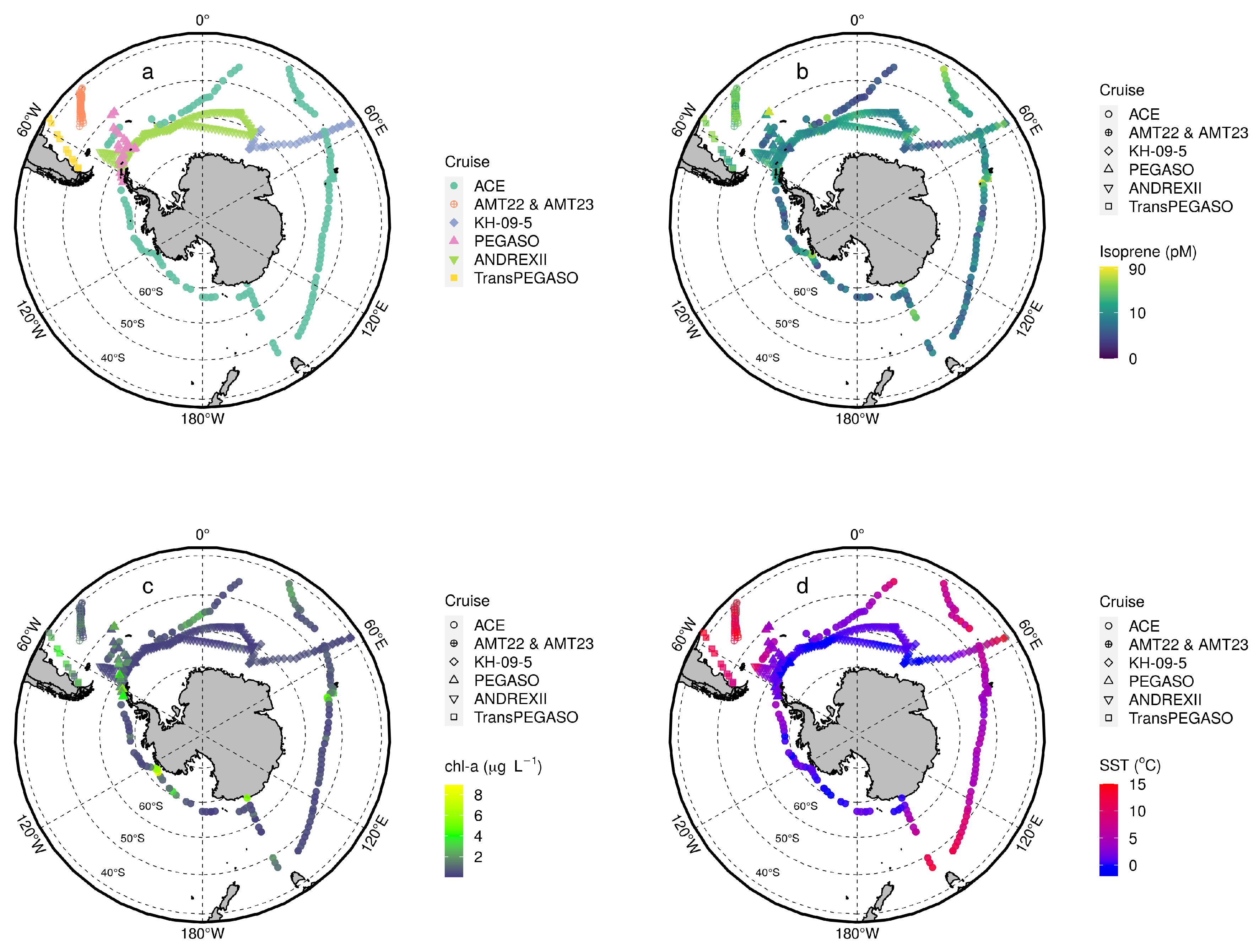
3.1. General Patterns of Isoprene Surface Concentration in the Southern Ocean

In Figure 1b, we show surface ocean isoprene concentration measurements from all cruises (see also Table A1). Overall, higher isoprene concentrations occurred in waters with high temperature (Figure 1d) and chlorophyll-a (Figure 1c). The highest concentrations (close to 100 pM) were measured during PEGASO in the phytoplankton bloom north of South Georgia Islands [22,23]. In contrast, concentrations as low as 1–2 pM occurred in waters with low chlorophyll-a content during ACE and PEGASO (Figure 1b,c and Figure 2b). Concentrations of isoprene during PEGASO show the largest variability among cruises, which is due to the sampling strategy of this cruise, which aimed at blooming waters and contrasting conditions (Table A1). The rest of the cruises showed concentrations that rarely exceeded 50 pM (Figure 1b).
In the combined dataset, a hump of higher isoprene concentrations (>20 pM) is observed at water temperatures of ≈15 C and a latitude 40–45 S (Figure 2a–d). This same pattern was already described by Ooki et al. [13] and was attributed to the temperature range associated with phytoplankton blooms in transitional and subpolar waters, and consequently being coincident with the Subantarctic front. This latitudinal band, which covers a large area, is important for isoprene emission, more so than coastal or near island, biologically rich sites like the South Georgia and Kerguelen blooms (Figure 2b,d). In most of the rest of the SO, characterized by chlorophyll-poorer waters, isoprene concentrations are low (<15 pM). Consequently, we suggest that the 40–45 S waters would be a good target for future experimental studies aiming to decipher isoprene production, cycling, and emission rates and their seasonality in the SO.

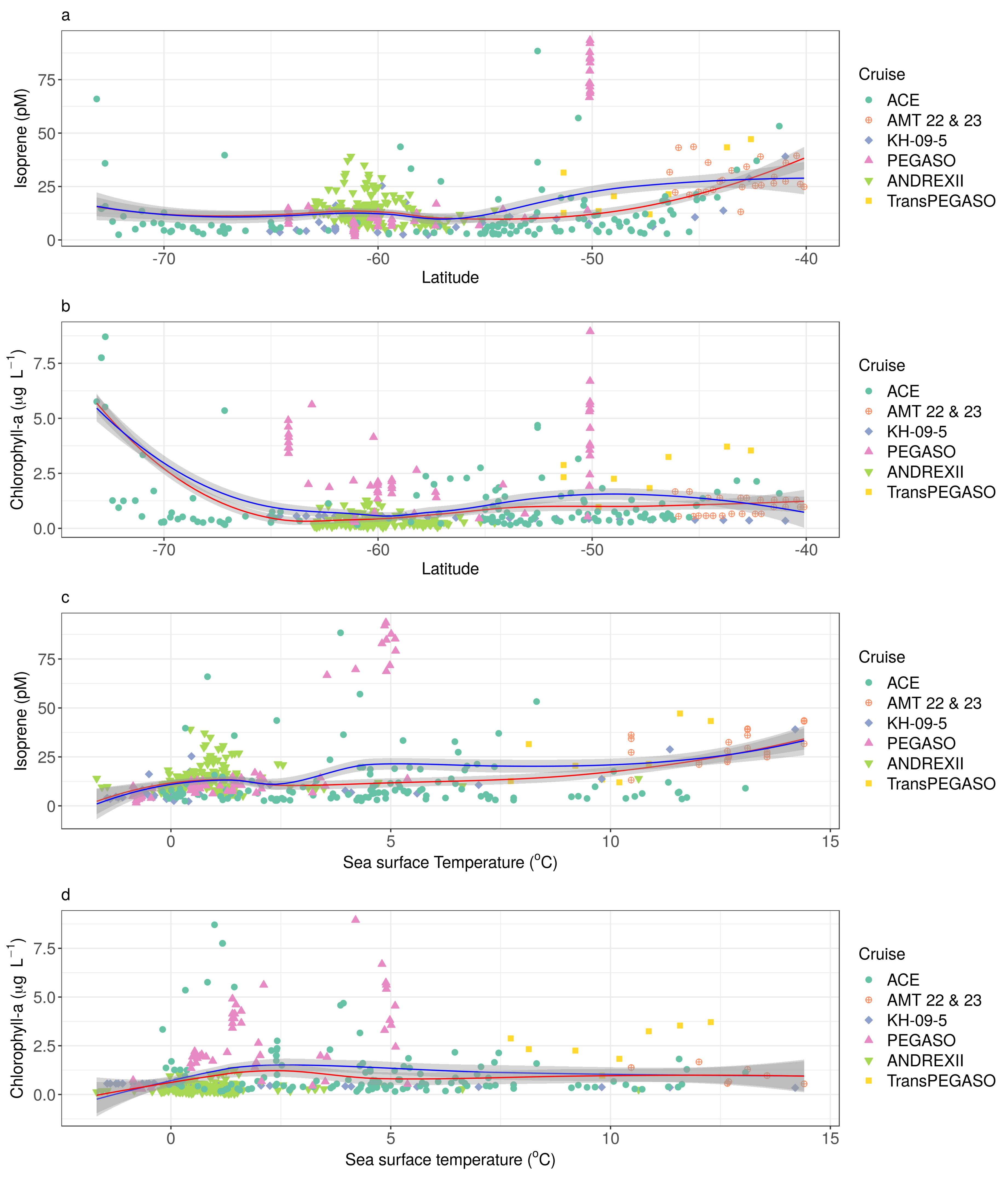
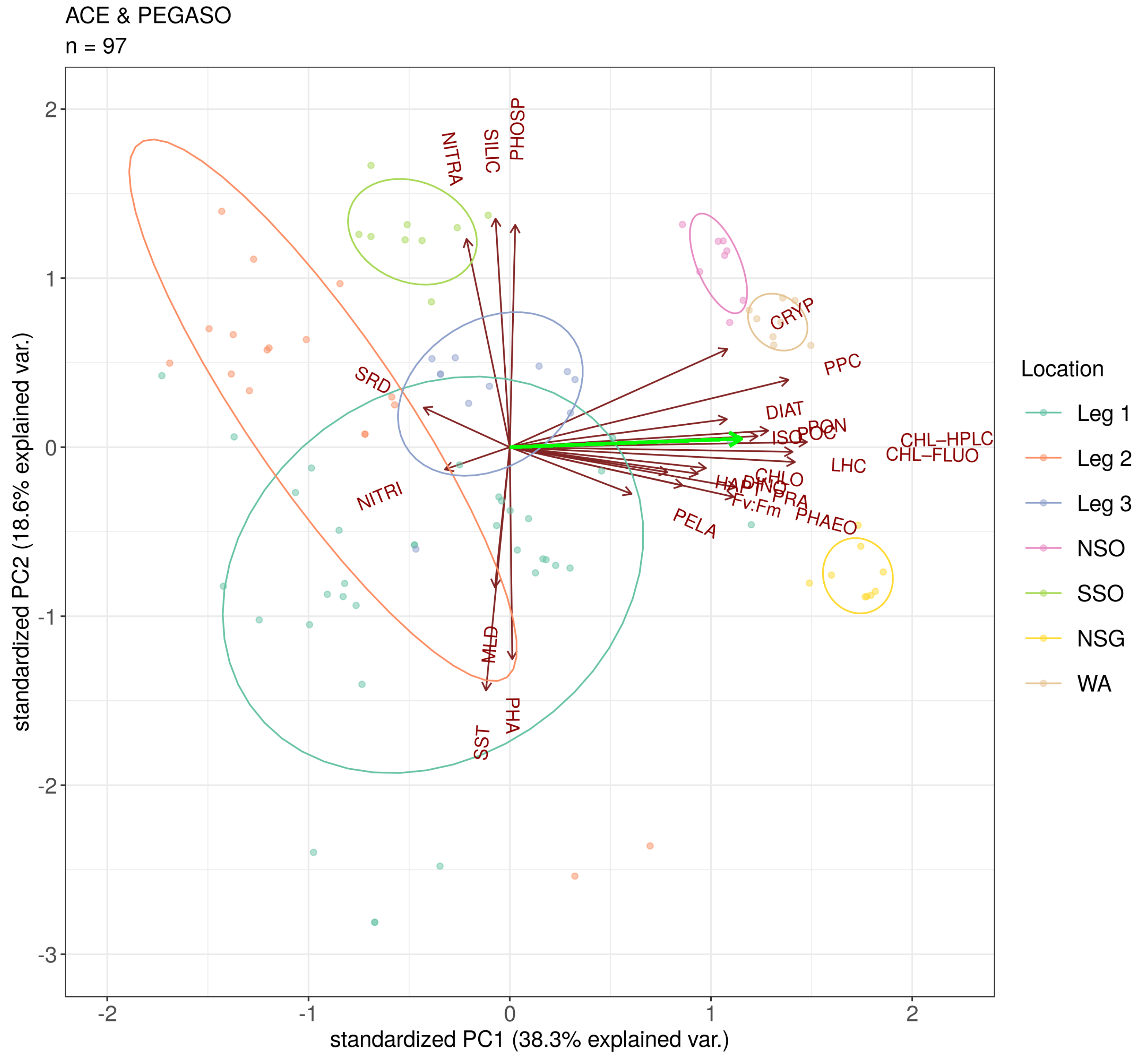
3.2. Drivers of Isoprene Concentration in the Southern Ocean

Isoprene was significantly correlated with CHL-FLUOR and CHL-HPLC ( r 2 = 0.38 and 0.48, respectively) across the PEGASO and ACE cruises (Table 1). It also correlated positively with total light-harvesting and total photoprotective carotenoids (LHC and PPC, respectively; r 2 = 0.45 in both cases). Positive correlation extended to all phytoplankton groups analyzed, particularly diatoms (DIAT), Phaeocystis-like haptophytes (PHAEO), and dinoflagellates (DINO) ( r 2 = 0.26, 0.26, and 0.23, respectively). Among the other biological and environmental descriptors, isoprene significantly correlated with F v : F m , POC, and PON ( r 2 = 0.31, 0.25, and 0.34, respectively) and showed negative but weak significant correlation with nitrite and silicate concentrations ( r 2 = 0.05 and 0.03, respectively).
A multivariate PCA was performed with PEGASO and ACE data to visualize combinations of variables that better explained isoprene patterns as well as the differences between the visited errorregions (Figure 3). PC1 + PC2 explained 57% of the total variance (Figure 3). Essentially, PC1 can be regarded as a “productivity” axis, contributed positively by phytoplankton-related variables and with negative weak contributions by SRD and nitrite. In contrast, PC2 represents the physico-chemical environment, with SST and MLD on one side and macronutrients on the opposite side. Note that the abundance of prokaryotic heterotrophs is strictly aligned with SST. Isoprene contributes only to PC1, and aligns positively with proxies of phytoplankton biomass (chlorophyll-a, POC, PON) and the biomass shares of most phytoplankton taxa, particularly diatoms. It also aligns positively with light-harvesting capacity (LHC) and F v : F m , which varies with phytoplankton taxonomy [44], but is also a powerful indicator of the efficiency of photosystem II in phytoplankton [32,33,45]. In the overall Fe-limited Southern Ocean, spots of Fe availability, generally associated with divergence zones near islands, show increases in productivity, phytoplankton biomass and F v : F m [23,46,47,48,49]. As mentioned above, these are zones of high isoprene too. Isoprene is orthogonal to PC2, meaning that it does not contribute to the proportion of the total variance explained by this component. This confirms what the paired regressions had indicated: isoprene shows no proportionality, either positive or negative, to macronutrients, SST, MLD, or PHA. In other oceans, phytoplankton productivity is largely dictated by macronutrient availability; the SO, however, is generally macronutrient-replete but limited in micro-nutrient Fe, essential for building photosynthetic machinery [50,51]. Therefore, macronutrients do not contribute to the variances of phytoplankton biomass proxies and isoprene concentration. SST is also orthogonal to isoprene; previous studies had already reported that SST does not show any covariance with isoprene concentration but it rather defines regions of distinct isoprene variability [13,15]. Regarding PHA, even though it has been demonstrated that heterotrophic prokaryotes can both produce [52] and consume [10] isoprene, their total abundance is not a significant driver of isoprene concentration. It must be noted that total prokaryotic heterotrophic abundance does not necessarily parallel prokaryotic activity, less so the activity of specific phyla potentially involved in isoprene production or consumption.
The sampling sites from PEGASO and ACE are spread over the 2D field defined by PC1 and PC2, according to the contribution of the two components to the site’s total variance. PC1 splits the sampling sites between the high isoprene, chlorophyll-rich blooms of PEGASO (SG, WA, and NSO) plus a few stations near Kerguelen visited during ACE (leg 1), and the low isoprene, chlorophyll-poor waters generally encountered during ACE and in PEGASO SSO. PC2 distributed sampling sites essentially according to SST, with higher SST and lower macronutrient concentrations encountered near Hobart in the end of ACE leg 1 and the beginning of ACE leg 2, and the lowest SST, associated with high macronutrient concentrations, located near the Antarctic coasts during the two cruises.
Considering the paired regressions and the PCA, there is a clear pattern in the control mechanisms of isoprene concentration in the SO, which is largely associated with phytoplankton abundance and biological productivity (Figure 3). This correlation is mainly driven by the measurements from PEGASO, a cruise that purposely sampled regions of high productivity, accompanied by high isoprene concentrations. Conversely, ACE had a much less targeted cruise track, more representative of the background conditions of the SO, and the isoprene concentrations encountered were persistently low, except for a few sampling sites at lower latitudes, near the Kergelen-Heard islands, or right at the Antarctic continental coast (Figure 1b).
The link of isoprene concentration to overall phytoplankton abundance has been repeatedly reported in previous works in the Southern Ocean [4,53,54], and is not surprising given that isoprene production has been observed and quantified in laboratory conditions for many phytoplankton species [2,3,55,56]. Diatoms, which are common bloom formers, have been proposed as the main producers of isoprene in the global ocean [17]. In this work, of the phytoplankton taxonomic indicators, diatoms (DIAT) showed the strongest correlation to isoprene concentrations. However, most phytoplankton groups were positively correlated to isoprene too, including known strong isoprene producers like dinoflagellates, haptophytes, and cryptophytes [14], but also including Phaeocystis-like haptophytes, which have not been reported to be isoprene producers [57]. This is likely due to the tight covariation of most phytoplankton taxa throughout large sections of the cruise tracks.
Hackenberg et al. [15] proposed a relationship between isoprene and PPC that was even better than that with chlorophyll-a for the global ocean. As PPC are indicators of photoacclimatation of phytoplankton to high SRD, the tight relationship was suggestive of a photoprotective function of isoprene, or at least of isoprene being a by-product of photoprotection in phytoplankton. In land vegetation, isoprene emission as a photoprotective mechanism has been demonstrated [58]. In the ocean, however, although a connection between isoprene and phytoplankton light stress has been speculated [2,55,56,59], involvement in a photoprotective mechanism has not yet been proved [15]. Our observed correlation between isoprene and PPC across the Southern Ocean (Table 1) could support such a photoprotective role; however, a similar correlation was found with LHC, and none of the two were better than the correlation with CHL-HPLC. In the PCA, PPC were strongly aligned with all indicators of phytoplankton biomass (Figure 3) and, most importantly, they did not align with SRD, which had a minor and opposite-to-PPC contribution to PC1. Therefore, we believe that the variability of PPC across our Southern Oceans samples was less indicative of photoacclimation or photoprotection and essentially driven by total phytoplankton abundance. The ratio PPC/LHC normalizes photoprotective capacity with respect to the light harvesting one, hence being more appropriate to asses photoacclimation; nonetheless, isoprene concentration only weakly correlated to PPC/LHC ( r 2 = 0.16, Table 1). Even though we cannot discard that isoprene may be involved in phytoplankton photoprotection mechanisms, or be a by-product of it, our results do not provide any evidence for it.

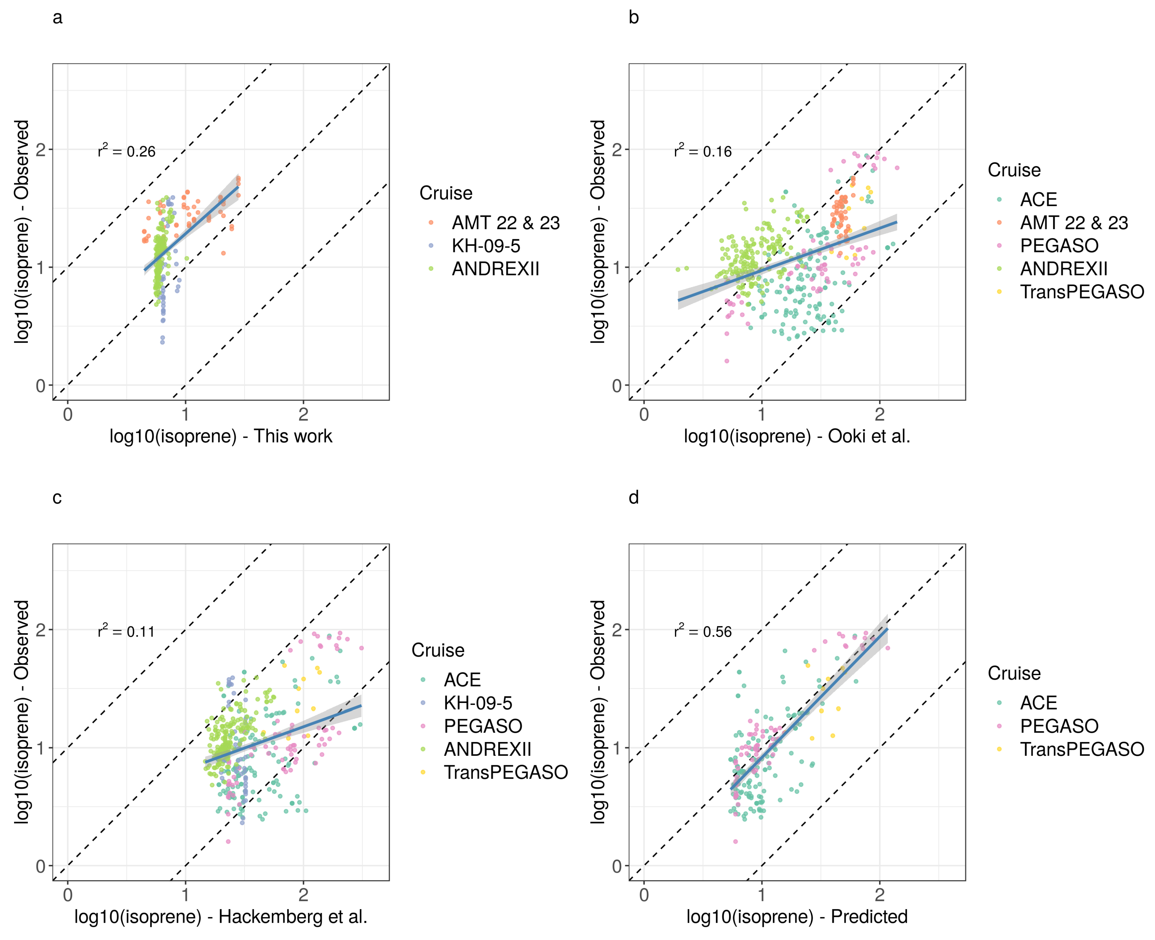
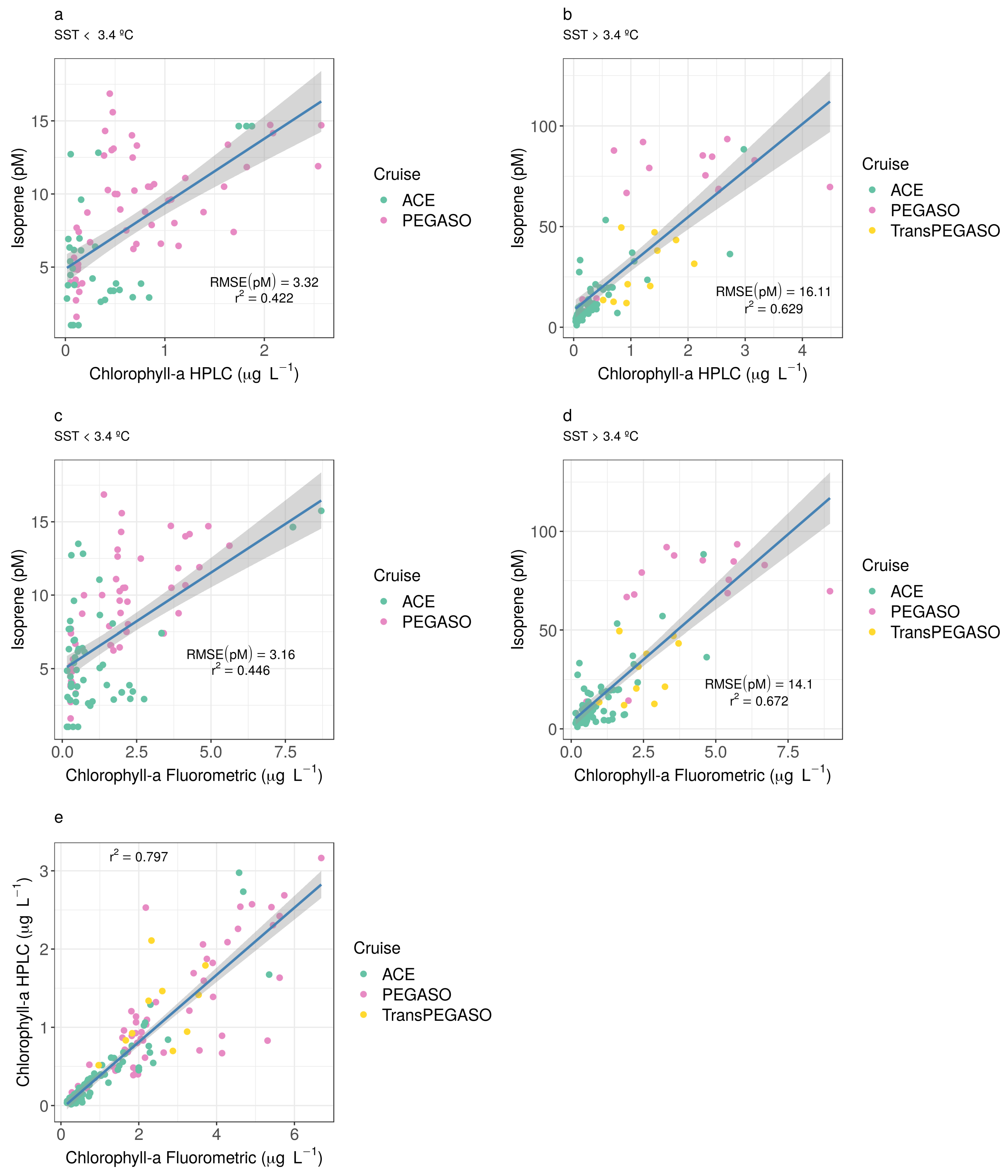
3.3. The Predictive Capacity of Chlorophyll-a and Sea Surface Temperature to Isoprene Concentration in the Southern Ocean

The ability of simple models to predict isoprene concentration in surface waters of the oceans has been widely discussed by Booge et al. [14] and Hackenberg et al. [15]. The global dataset of isoprene concentrations in the surface ocean is still quite poor, challenging the creation of simple statistical models of global applicability. The published attempts [13,15] agree that chlorophyll-a and sea surface temperature are the best statistical predictors of isoprene concentrations, although other variables like other pigments, nutrients, or light hold potential to improve the models [9,15,59]. Despite the high number of experimental approaches attempting to study the production and concentration levels of isoprene in laboratory conditions [2,3,14,55], only a few publications have tried to model isoprene concentrations using field data [13,15,57,60,61].
Exploration of isoprene to chl-a relationships according to SST regimes, following the work in [13,15], rendered 3.4 C as the SST break point that allowed to explain the largest portion of the isoprene concentration variance in PEGASO, ACE, and TransPEGASO (Figure A2a–d; Table 2). This break point agrees with that proposed by Ooki et al. [13] for Arctic and Antarctic waters (3.3 C). The fact that the resulting dual regression model is based on CHL-FLUO and SST makes it comparable to the other existing models and can be easily implemented on remote sensing measurements. Furthermore, SST and CHL-FLUO are typically sampled on oceanographic cruises, making the application of these relationships feasible to future datasets to test and improve their predictive capacity.
We examined the misfit between our model predictions and observations as a function of the magnitude of the predictor variables (CHL-FLUO and CHL-HPLC) (Figure A1). For both chlorophyll-a variables, the misfit was smaller at SST < 3.4 C than at SST > 3.4 C, which is due to the boader range into higher isoprene concentrations at SST > 3.4 C. The model tended to overestimate higher isoprene concentrations as chlorophyll-a increases in both SST regimes, and underestimate lower isoprene concentrations at low chlorophyll-a concentrations.
To compare the predictive performance of our model with the other statistical models suggested to date [13,15], we applied each of the models to the measurements which were not used for their development (Figure 4). We only used CHL-FLUO because this is the chl-a used in the published models, and there are no CHL-HPLC data available for the rest of cruises. Our model predictions generally overestimated observations for the AMT, KH-09-05, and ADREXII cruises, and the fit was weak ( r 2 = 0.26), but the slope was nearly 1 (Figure 4a). The overall fit to the data used to develop the model (developed from CHL-FLUO) was r 2 = 0.56 (Figure 4d). Conversely, the model of Ooki et al. [13] (cruise KH-09-5) on the AMT, TransPEGASO, PEGASO, ACE, and ANDREXII data gave a slope much lower than 1, a weaker fit ( r 2 = 0.11), and severely underestimated many isoprene measurements (Figure 4b). The model of Hackenberg et al. [15] did not perform any better ( r 2 = 0.16, slope < < 1) on the data from KH-09-05, TransPEGASO, PEGASO, ACE, and ANDREXII, underestimating most of the observations (Figure 4c).
The cross-comparison between statistical models reveals how challenging it is to find a simple model with good performance in an oceanic region as heterogeneous as the SO. An explanation why our model performs better than the other two models predicting isoprene concentrations from other cruises may lay in the broader geographic span and wider chlorophyll-a range (Figure 5) of PEGASO and ACE together. The AMT cruises [15] reached a maximum southern latitude of 50 S, without making any isoprene measurements in coastal areas or island blooms. Ooki et al. [13] pooled together Arctic and Antarctic data according to their SST despite the differences between the two regions in terms of phytoplankton taxa and environmental variables. Added to this need for a good data coverage of the SO, there is the difficulty of harmonizing the observations obtained from different cruises, methods, and operators. We compared models based on CHL-FLUO because this was available from PEGASO, TransPEGASO, ACE, KH-05-05, and the AMTs. On ANDREXII, however, chlorophyll-a concentrations were recorded with a sensor that had been calibrated against a solution prepared with pure chlorophyll-a. In the SO, Turner fluorometric measurements render CHL-FLUO concentrations that typically are more than twice the CHL-HPLC concentrations (Figure A2e), which can be considered close to pure chlorophyll-a. Therefore, the isoprene vs. chlorophyll-a slope of ANDREXII was higher than those of the other cruises, and it can be anticipated that, should CHL-FLUO had been available from that cruise too, our model validation would have given a better fit. Recently, Rodríguez-Ros et al. [43] developed a statistical model to estimate isoprene concentrations based on chlorophyll-a and sea surface temperature retrieved from satellite (MODIS Aqua) matchups to the isoprene observations. The advantage of this remote sensing approach is that it overcomes the aforementioned limitations of non-harmonized predictor data from diverse origins. Remote sensing has its own limitations, particularly in the cloudy SO, but it offers a promising alternative to studies based purely on field measurements.
In summary, our results support the idea that the complexity of the SO, with marked frontal zones and ephemeral or persistent presence of sea ice, land, and ice shelf coastlines, constitutes a challenge for ecological and biogeochemical model development of any kind [62], and particularly for trace gases. We have shown that, beyond an isoprene-rich band around 40 S, there is a background of low isoprene concentrations (1–2 pM) on top of which local peaks occur in shelf, polynya, and coastal waters, and island-associated blooms where phytoplankton communities are not iron-limited [48,50,51]. Future efforts aiming to comprehensively describe isoprene distribution and cycling in the Southern Ocean should consist of a combination of the PEGASO and the ACE approaches, that is, a combination of measurements over the large low-productivity areas, across biological and physical boundaries [62] as well as targeting for contrasting upwelling and blooming spots at different statges of bloom development [63].

Author Contributions

Conceptualization, R.S. and P.R.-R.; methodology, P.R.-R., P.C., and R.S.; validation, P.R.-R. and R.S.; formal analysis, P.R.-R., P.C., C.M.R., S.-J.R., C.H., S.N., and R.S.; investigation, P.R.-R., C.M.R., and R.S.; data curation, P.C., C.M.R., P.R.-R., M.E., M.M.S., and R.S.; writing—original draft preparation, P.R.-R. and R.S.; writing—review and editing, C.M.R., C.H., S.-J.R., M.E., and M.M.S.; visualization, P.R.-R. All authors have read and agreed to the published version of the manuscript.

Funding

This research was supported by the Spanish Ministry of Economy and Competitiveness through project PEGASO (CTM2012–37615) to R.S., and by the Swiss Polar Institute and Ferring Pharmaceuticals through project SORPASSO–ACE#8 to R.S. and project ACE#1 to David Antoine (Remote Sensing and Satellite Research Group, Curtin University) and Sandy Thomalla (Southern Ocean Carbon and Climate Observatory, Council for Scientific and Industrial Research (CSIR) and Marine Research Institute, University of Cape Town). It was also partially funded by the Australian Government through the Australian Research Council’s Discovery Projects funding scheme (project DP160103387) and South African CSIR Parliamentary Grant (SNA2011112600001). Project ACE#1 was also supported by CSIR Southern Ocean Carbon and Climate Observatory (SOCCO) programme. P.R.-R. was supported by a “la Caixa” Foundation PhD Fellowship (2015–2019).

Acknowledgments

Members of the ACE#1 research team are greatly acknowledged for providing data and technical support. PRR would like to thank Martí Galí from the Barcelona Supercomputing Centre for his advice with the statistical analysis and data visualization. We are grateful to the British Oceanographic Data Centre (BODC). We would like to thank to Miguel Cabrera, Laura Carrillo, Encarna Borrull and Carolina Antequera (ICM-CSIC) for flow citometry analyses, Mikhail Emelianov (ICM-CSIC) for mixed layer depth data, Nicolas Cassar and Yajuan Lin (Duke University) for sea surface temperature measurements, and Marina Zamanillo (ICM-CSIC) for computing solar radiation dose data and collecting flow citometry samples. We also want to thank the captains, officers and crew of RV Hespérides and RV Akademik Tryoshnikov, to the ACE chief Scientist David Walton, engineers of the Marine Technology Unit (CSIC) and research colleagues for their support and help during the cruises. Data of this work can be found at the Zenodo repository (https://doi.org/10.5281/zenodo.3773972). This research is part of POLARCSIC (https://polarcsic.es/) activities.

Conflicts of Interest

The authors declare no conflicts of interest.

Appendix A. Summary of Compiled Cruise Variables

Table A1. Surface isoprene concentration measurements (0–10 m depth) in the Southern Ocean (>40 S) along the research cruises used for model comparisons (Figure 1): PEGASO, TransPEGASO, ACE Expedition, AMT22, AMT23, KH-09-5, and ANDREXII. For more details, see Rodríguez-Ros et al. 2020.
Isoprene (pM)Chlorophyll-a ( μ g L 1 )Sea Surface Temperature ( C)Southern Ocean AreaCruise
Mean (Min–Max)Mean (Min–Max)Mean (Min–Max)
10.7 (2.1–88.4)1.46 (0.15–8.70 )4.16 (−0.18–13.06)SO CircumnavigationACE
22.4 (1.6–93.5)2.42 (0.28–8.95)1.45 (−0.87–5.38)SO and Weddell SeaPEGASO
25.3 (12.0–49.5)2.59 (0.97–3.71)9.97 (7.73–12.28)Southwestern Atlantic SelfTransPEGASO
29.0 (13.1–57.1)0.97 (0.55–1.67)12.68 (10.46–14.40)SO + South Atlantic OceanAMT23 & AMT22
9.5 (2.3–39.0)0.49 (0.34–0.56)1.82 (−1.45–14.2)SO + South Indian OceanKH-09-5
13.5 (4.8–39.1)0.33 (0.02–1.27)0.91 (−1.68–10.63)SO + South Atlantic OceanANDREXII

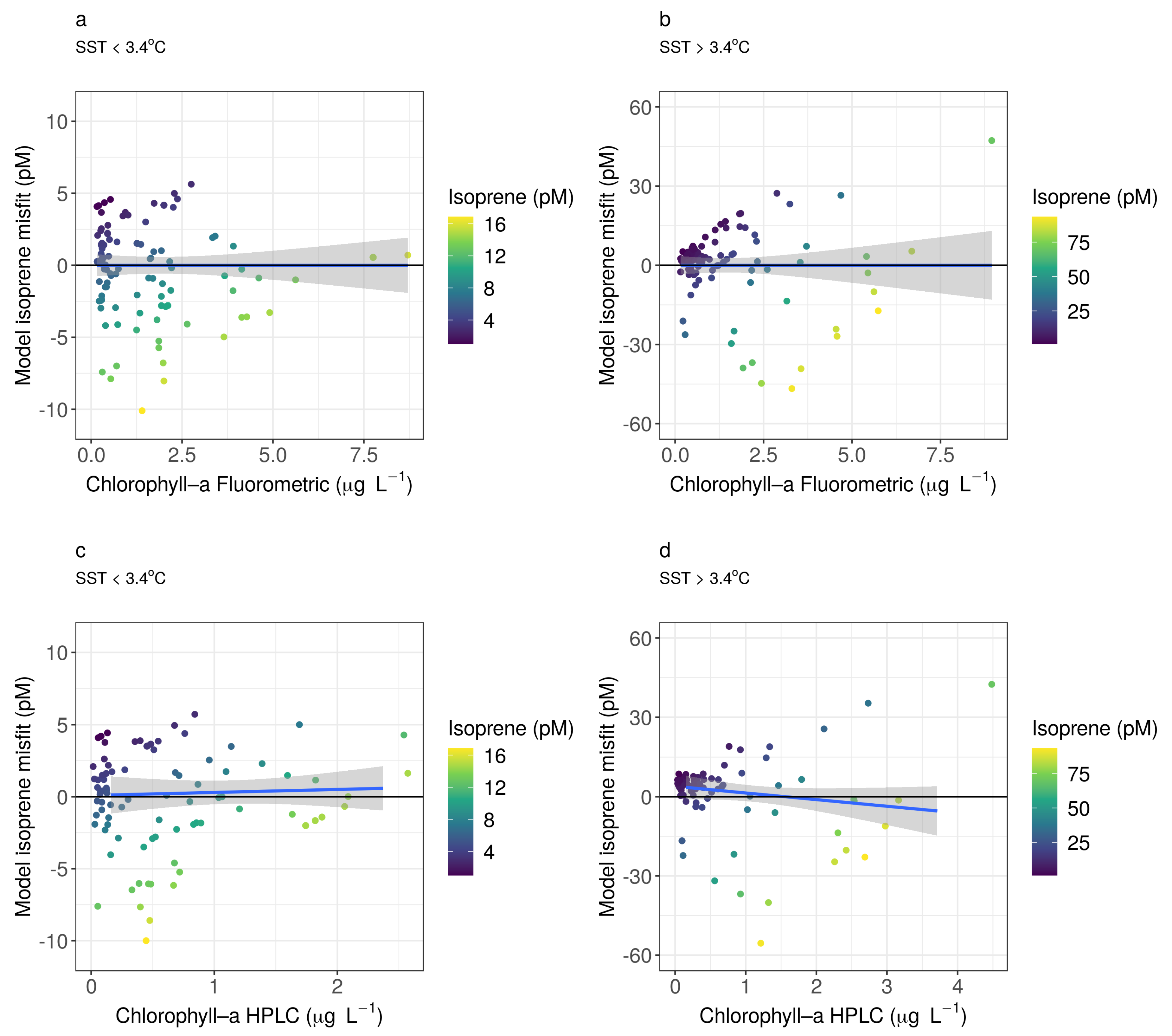
Appendix B. Residuals

Figure A1. Scatterplot of misfit (residuals) among observed and predicted isoprene concentration values from PEGASO and ACE cruises cruises versus chlorophyll-a levels (Fluorometric: a,b; and HPLC: c,d).
Atmosphere 11 00556 g0a1

Appendix C. Statistical Relationships between Isoprene Concentration and Chlorophyll-a Concentration and Sea Surface Temperature

Figure A2. (a,b) Isoprene model based on CHLA-FLUO with the shifting regime based on a SST threshold of 3.4 C. (c,d) Isoprene model based on CHLA-HPLC with the shifting regime based on a SST threshold of 3.4 C. (e) CHLA-HPLC vs CHLA-FLUO. For these plots only data from TransPEGASO, PEGASO and ACE cruises were used (Figure 1, Table A1). RMSE = Root Mean Square Error (see Equation (2)).
Atmosphere 11 00556 g0a2

References

  1. Carpenter, L.J.; Archer, S.D.; Beale, R. Ocean-atmosphere trace gas exchange. Chem. Soc. Rev. 2012, 41, 6473–6506. [Google Scholar] [CrossRef] [PubMed]
  2. Shaw, S.L.; Chisholm, S.W.; Prinn, R.G. Isoprene production by Prochlorococcus, a marine cyanobacterium, and other phytoplankton. Mar. Chem. 2003, 80, 227–245. [Google Scholar] [CrossRef]
  3. Exton, D.; Suggett, D.J.; McGenity, T.J.; Steinke, M. Chlorophyll-normalized isoprene production in laboratory cultures of marine microalgae and implications for global models. Limnol. Oceanogr. 2013, 58, 1301–1311. [Google Scholar] [CrossRef] [Green Version]
  4. Meskhidze, N.; Nenes, A. Phytoplankton and cloudiness in the Southern Ocean. Science 2006, 314, 1419–1423. [Google Scholar] [CrossRef] [PubMed] [Green Version]
  5. Arnold, S.; Spracklen, D.; Williams, J.; Yassaa, N.; Sciare, J.; Bonsang, B.; Gros, V.; Peeken, I.; Lewis, A.; Alvain, S.; et al. Evaluation of the global oceanic isoprene source and its impacts on marine organic carbon aerosol. Atmos. Chem. Phys. 2009, 9, 1253–1262. [Google Scholar] [CrossRef] [Green Version]
  6. Vallina, S.; Simó, R.; Gassó, S.; de Boyer-Montégut, C.; Del Río, E.; Jurado, E.; Dachs, J. Analysis of a potential “solar radiation dose–dimethylsulfide–cloud condensation nuclei” link from globally mapped seasonal correlations. Glob. Biogeochem. Cycles 2007, 21, 0886–6236. [Google Scholar]
  7. Dani, K.S.; Loreto, F. Trade-off between dimethyl sulfide and isoprene emissions from marine phytoplankton. Trends Plant Sci. 2017, 22, 361–372. [Google Scholar]
  8. Luo, G.; Yu, F. A numerical evaluation of global oceanic emissions of α-pinene and isoprene. Atmos. Chem. Phys. 2010, 10, 2007–2015. [Google Scholar] [CrossRef] [Green Version]
  9. Booge, D.; Schlundt, C.; Bracher, A.; Endres, S.; Zäncker, B.; Marandino, C.A. Marine isoprene production and consumption in the mixed layer of the surface ocean—A field study over two oceanic regions. Biogeosciences (BG) 2018, 15, 649–667. [Google Scholar]
  10. Alvarez, L.A.; Exton, D.A.; Timmis, K.N.; Suggett, D.J.; McGenity, T.J. Characterization of marine isoprene-degrading communities. Environ. Microbiol. 2009, 11, 3280–3291. [Google Scholar] [CrossRef]
  11. Ciuraru, R.; Fine, L.; Pinxteren, M.v.; D’Anna, B.; Herrmann, H.; George, C. Unravelling new processes at interfaces: Photochemical isoprene production at the sea surface. Environ. Sci. Technol. 2015, 49, 13199–13205. [Google Scholar] [CrossRef] [PubMed]
  12. Brüggemann, M.; Hayeck, N.; George, C. Interfacial photochemistry at the ocean surface is a global source of organic vapors and aerosols. Nat. Commun. 2018, 9, 2101. [Google Scholar] [CrossRef] [PubMed]
  13. Ooki, A.; Nomura, D.; Nishino, S.; Kikuchi, T.; Yokouchi, Y. A global-scale map of isoprene and volatile organic iodine in surface seawater of the Arctic, Northwest Pacific, Indian, and Southern Oceans. J. Geophys. Res. Ocean. 2015, 120, 4108–4128. [Google Scholar] [CrossRef] [Green Version]
  14. Booge, D.; Marandino, C.A.; Schlundt, C.; Palmer, P.I.; Schlundt, M.; Atlas, E.L.; Bracher, A.; Saltzman, E.S.; Wallace, D.W. Can simple models predict large-scale surface ocean isoprene concentrations? Atmos. Chem. Phys. 2016, 16, 11807–11821. [Google Scholar] [CrossRef] [Green Version]
  15. Hackenberg, S.; Andrews, S.; Airs, R.; Arnold, S.; Bouman, H.; Brewin, R.; Chance, R.; Cummings, D.; Dall’Olmo, G.; Lewis, A.; et al. Potential controls of isoprene in the surface ocean. Glob. Biogeochem. Cycles 2017, 31, 644–662. [Google Scholar] [CrossRef]
  16. Palmer, P.I.; Shaw, S.L. Quantifying global marine isoprene fluxes using MODIS chlorophyll observations. Geophys. Res. Lett. 2005, 32. [Google Scholar] [CrossRef] [Green Version]
  17. Dani, K.S.; Benavides, A.M.S.; Michelozzi, M.; Peluso, G.; Torzillo, G.; Loreto, F. Relationship between isoprene emission and photosynthesis in diatoms, and its implications for global marine isoprene estimates. Mar. Chem. 2017, 189, 17–24. [Google Scholar] [CrossRef]
  18. Zindler, C.; Marandino, C.A.; Bange, H.W.; Schütte, F.; Saltzman, E.S. Nutrient availability determines dimethyl sulfide and isoprene distribution in the eastern Atlantic Ocean. Geophys. Res. Lett. 2014, 41, 3181–3188. [Google Scholar] [CrossRef] [Green Version]
  19. Kameyama, S.; Tanimoto, H.; Inomata, S.; Tsunogai, U.; Ooki, A.; Takeda, S.; Obata, H.; Tsuda, A.; Uematsu, M. High-resolution measurement of multiple volatile organic compounds dissolved in seawater using equilibrator inlet–proton transfer reaction-mass spectrometry (EI–PTR-MS). Mar. Chem. 2010, 122, 59–73. [Google Scholar] [CrossRef]
  20. Wohl, C.; Brown, I.; Kitidis, V.; Jones, A.E.; Sturges, W.T.; Nightingale, P.D.; Yang, M. Underway seawater and atmospheric measurements of volatile organic compounds in the Southern Ocean. Biogeosciences 2020, 2020, 2593–2619. [Google Scholar] [CrossRef]
  21. Dall’Osto, M.; Ovadnevaite, J.; Paglione, M.; Beddows, D.C.; Ceburnis, D.; Cree, C.; Cortés, P.; Zamanillo, M.; Nunes, S.O.; Pérez, G.L.; et al. Antarctic sea ice region as a source of biogenic organic nitrogen in aerosols. Sci. Rep. 2017, 7, 6047. [Google Scholar] [CrossRef] [PubMed] [Green Version]
  22. Nunes, S.; Latasa, M.; Delgado, M.; Emelianov, M.; Simó, R.; Estrada, M. Phytoplankton community structure in contrasting ecosystems of the Southern Ocean: South Georgia, South Orkneys and western Antarctic Peninsula. Deep Sea Res. Part I Oceanogr. Res. Pap. 2019, 151, 103059. [Google Scholar] [CrossRef] [Green Version]
  23. Zamanillo, M.; Ortega-Retuerta, E.; Nunes, S.; Estrada, M.; Sala, M.M.; Royer, S.J.; López-Sandoval, D.C.; Emelianov, M.; Vaqué, D.; Marrasé, C.; et al. Distribution of transparent exopolymer particles (TEP) in distinct regions of the Southern Ocean. Sci. Total Environ. 2019, 691, 736–748. [Google Scholar] [CrossRef] [PubMed] [Green Version]
  24. Henry, T.; Robinson, C.; Haumman, F.; Thomas, J.; Hitchings, J.; Schuback, N.; Tsukernik, M.; Leonard, K. Physical and biogeochemical oceanography data from Conductivity, Temperature, Depth (CTD) rosette deployments during the Antarctic Circumnavigation Expedition (ACE). ACE Exped. Data-Sets 2020. [Google Scholar] [CrossRef]
  25. Yentsch, C.S.; Menzel, D.W. A method for the determination of phytoplankton chlorophyll and phaeophytin by fluorescence. In Deep Sea Research and Oceanographic Abstracts; Elsevier: Amsterdam, The Netherlands, 1963; Volume 10, pp. 221–231. [Google Scholar]
  26. Antoine, D.; Thomalla, S.; Berliner, D.; Little, H.; Moutier, W.; Olivier-Morgan, A.; Robinson, C.; Ryan-Keogh, T.; Schuback, N. Phytoplankton pigment concentrations of seawater sampled during the Antarctic Circumnavigation Expedition (ACE) during the Austral Summer of 2016/2017. Zenodo 2019. [Google Scholar] [CrossRef]
  27. Rodriguez, F.; Varela, M.; Zapata, M. Phytoplankton assemblages in the Gerlache and Bransfield Straits (Antarctic Peninsula) determined by light microscopy and CHEMTAX analysis of HPLC pigment data. Deep Sea Res. Part II Top. Stud. Oceanogr. 2002, 49, 723–747. [Google Scholar] [CrossRef]
  28. Zapata, M.; Rodríguez, F.; Garrido, J.L. Separation of chlorophylls and carotenoids from marine phytoplankton: A new HPLC method using a reversed phase C8 column and pyridine-containing mobile phases. Mar. Ecol. Prog. Ser. 2000, 195, 29–45. [Google Scholar] [CrossRef] [Green Version]
  29. Cook, S.S.; Whittock, L.; Wright, S.W.; Hallegraeff, G.M. Photosynthetic pigment and genetic differences between two Southern Ocean morphotypes of Emiliania huxleyi (Haptophyta) 1. J. Phycol. 2011, 47, 615–626. [Google Scholar] [CrossRef]
  30. Higgins, H.W.; Wright, S.W.; Schluter, L. Quantitative Interpretation of Chemotaxonomic Pigment Data; Cambridge University Press: Cambridge, UK, 2011. [Google Scholar]
  31. Cassar, N.; Wright, S.W.; Thomson, P.G.; Trull, T.W.; Westwood, K.J.; de Salas, M.; Davidson, A.; Pearce, I.; Davies, D.M.; Matear, R.J. The relation of mixed-layer net community production to phytoplankton community composition in the Southern Ocean. Glob. Biogeochem. Cycles 2015, 29, 446–462. [Google Scholar] [CrossRef]
  32. Kolber, Z.S.; Prášil, O.; Falkowski, P.G. Measurements of variable chlorophyll fluorescence using fast repetition rate techniques: Defining methodology and experimental protocols. Biochim. Biophys. Acta (BBA)-Bioenerg. 1998, 1367, 88–106. [Google Scholar] [CrossRef] [Green Version]
  33. Royer, S.J.; Mahajan, A.; Galí, M.; Saltzman, E.; Simó, R. Small-scale variability patterns of DMS and phytoplankton in surface waters of the tropical and subtropical Atlantic, Indian, and Pacific Oceans. Geophys. Res. Lett. 2015, 42, 475–483. [Google Scholar] [CrossRef] [Green Version]
  34. Ryan-Keogh, T.; Robinson, C. Phytoplankton Photophysiology Utilities: A Python Toolbox for the standardisation of processing active chlorophyll fluorescence data. Front. Mar. Sci. Aquat. Physiol. 2020, submitted. [Google Scholar]
  35. Gasol, J.M.; Del Giorgio, P.A. Using flow cytometry for counting natural planktonic bacteria and understanding the structure of planktonic bacterial communities. Sci. Mar. 2000, 64, 197–224. [Google Scholar] [CrossRef] [Green Version]
  36. Hansen, H.; Grasshoff, K. Automated chemical analysis. In Methods of Seawater Analysis; Verlag Chemie Weinheim: Weinheim, Germany, 1983; pp. 347–379. [Google Scholar]
  37. Wolters, M. Determination of Silicate in Brackish or Seawater by Flow Injection Analysis. QuickChem Method 31-114-27-1-D; Methods Manual; Lachat Instruments: Milwaukee, WI, USA, 2002; 12p. [Google Scholar]
  38. Egan, L. Determination of Nitrate and/or Nitrite in Brackish or Seawater by Flow Injection Analysis. QuikChem Method 31-107-04-1-C; Lachat Instruments: Milwaukee, WI, USA, 2008. [Google Scholar]
  39. Grasshoff, K.; Kremling, K.; Ehrhardt, M. Methods of Seawater Analysis; John Wiley & Sons: Hoboken, NJ, USA, 2009. [Google Scholar]
  40. Schlitzer, R.; Anderson, R.F.; Dodas, E.M.; Lohan, M.; Geibert, W.; Tagliabue, A.; Bowie, A.; Jeandel, C.; Maldonado, M.T.; Landing, W.M.; et al. The GEOTRACES Intermediate Data Product 2017. Chem. Geol. 2018, 493, 210–223. [Google Scholar] [CrossRef]
  41. Wohl, C.; Capelle, D.; Jones, A.; Sturges, W.T.; Nightingale, P.D.; Else, B.G.; Yang, M. Segmented flow coil equilibrator coupled to a Proton Transfer Reaction Mass Spectrometer for measurements of a broad range of Volatile Organic Compounds in seawater. Ocean Sci. 2019, 15, 925–940. [Google Scholar] [CrossRef] [Green Version]
  42. RStudio Team. RStudio: Integrated Development Environment for R; RStudio, Inc.: Boston, MA, USA, 2015. [Google Scholar]
  43. Rodríguez-Ros, P.; Galí, M.; Cortés, P.; Robinson, C.M.; Antoine, D.; Wohl, C.; Yang, M.; Simó, R. Remote sensing retrieval of isoprene concentrations in the Southern Ocean. Under Rev.—Geophys. Res. Lett. 2020, in press. [Google Scholar] [CrossRef]
  44. Suggett, D.J.; Moore, C.M.; Hickman, A.E.; Geider, R.J. Interpretation of fast repetition rate (FRR) fluorescence: Signatures of phytoplankton community structure versus physiological state. Mar. Ecol. Prog. Ser. 2009, 376, 1–19. [Google Scholar] [CrossRef] [Green Version]
  45. Behrenfeld, M.J.; Boss, E. Beam attenuation and chlorophyll concentration as alternative optical indices of phytoplankton biomass. J. Mar. Res. 2006, 64, 431–451. [Google Scholar] [CrossRef]
  46. Gervais, F.; Riebesell, U.; Gorbunov, M.Y. Changes in primary productivity and chlorophyll a in response to iron fertilization in the Southern Polar Frontal Zone. Limnol. Oceanogr. 2002, 47, 1324–1335. [Google Scholar] [CrossRef] [Green Version]
  47. Holeton, C.L.; Nedelec, F.; Sanders, R.; Brown, L.; Moore, C.M.; Stevens, D.P.; Heywood, K.J.; Statham, P.J.; Lucas, C.H. Physiological state of phytoplankton communities in the Southwest Atlantic sector of the Southern Ocean, as measured by fast repetition rate fluorometry. Polar Biol. 2005, 29, 44–52. [Google Scholar] [CrossRef] [Green Version]
  48. Morris, P.J.; Sanders, R. A carbon budget for a naturally iron fertilized bloom in the Southern Ocean. Glob. Biogeochem. Cycles 2011, 25. [Google Scholar] [CrossRef] [Green Version]
  49. Ryan-Keogh, T.J.; Macey, A.I.; Nielsdóttir, M.C.; Lucas, M.I.; Steigenberger, S.S.; Stinchcombe, M.C.; Achterberg, E.P.; Bibby, T.S.; Moore, C.M. Spatial and temporal development of phytoplankton iron stress in relation to bloom dynamics in the high-latitude North Atlantic Ocean. Limnol. Oceanogr. 2013, 58, 533–545. [Google Scholar] [CrossRef]
  50. Moore, C.; Mills, M.; Arrigo, K.; Berman-Frank, I.; Bopp, L.; Boyd, P.; Galbraith, E.; Geider, R.; Guieu, C.; Jaccard, S.; et al. Processes and patterns of oceanic nutrient limitation. Nat. Geosci. 2013, 6, 701–710. [Google Scholar]
  51. Hoppe, C.; Klaas, C.; Ossebaar, S.; Soppa, M.A.; Cheah, W.; Laglera, L.; Santos-Echeandia, J.; Rost, B.; Wolf-Gladrow, D.; Bracher, A.; et al. Controls of primary production in two phytoplankton blooms in the Antarctic Circumpolar Current. Deep Sea Res. Part II Top. Stud. Oceanogr. 2017, 138, 63–73. [Google Scholar] [CrossRef] [Green Version]
  52. Fall, R.; Copley, S.D. Bacterial sources and sinks of isoprene, a reactive atmospheric hydrocarbon. Environ. Microbiol. 2000, 2, 123–130. [Google Scholar] [CrossRef] [Green Version]
  53. Wingenter, O.W.; Haase, K.B.; Strutton, P.; Friederich, G.; Meinardi, S.; Blake, D.R.; Rowland, F.S. Changing concentrations of CO, CH4, C5H8, CH3Br, CH3I, and dimethyl sulfide during the Southern Ocean Iron Enrichment Experiments. Proc. Natl. Acad. Sci. USA 2004, 101, 8537–8541. [Google Scholar]
  54. Moore, R.M. Methyl halide production and loss rates in sea water from field incubation experiments. Mar. Chem. 2006, 101, 213–219. [Google Scholar]
  55. Bonsang, B.; Gros, V.; Peeken, I.; Yassaa, N.; Bluhm, K.; Zöllner, E.; Sarda-Esteve, R.; Williams, J. Isoprene emission from phytoplankton monocultures: The relationship with chlorophyll-a, cell volume and carbon content. Environ. Chem. 2010, 7, 554–563. [Google Scholar] [CrossRef]
  56. Meskhidze, N.; Sabolis, A.; Reed, R.; Kamykowski, D. Quantifying environmental stress-induced emissions of algal isoprene and monoterpenes using laboratory measurements. Biogeosciences 2015, 12, 637–651. [Google Scholar] [CrossRef] [Green Version]
  57. Broadgate, W.J.; Liss, P.S.; Penkett, S.A. Seasonal emissions of isoprene and other reactive hydrocarbon gases from the ocean. Geophys. Res. Lett. 1997, 24, 2675–2678. [Google Scholar] [CrossRef]
  58. Sharkey, T.D.; Yeh, S. Isoprene emission from plants. Annu. Rev. Plant Biol. 2001, 52, 407–436. [Google Scholar] [CrossRef] [PubMed]
  59. Gantt, B.; Meskhidze, N.; Kamykowski, D. A new physically-based quantification of isoprene and primary organic aerosol emissions from the world’s oceans. Atmos. Chem. Phys. Discuss 2009, 9, 2933–2965. [Google Scholar] [CrossRef] [Green Version]
  60. Kurihara, M.; Kimura, M.; Iwamoto, Y.; Narita, Y.; Ooki, A.; Eum, Y.J.; Tsuda, A.; Suzuki, K.; Tani, Y.; Yokouchi, Y.; et al. Distributions of short-lived iodocarbons and biogenic trace gases in the open ocean and atmosphere in the western North Pacific. Mar. Chem. 2010, 118, 156–170. [Google Scholar]
  61. Kurihara, M.; Iseda, M.; Ioriya, T.; Horimoto, N.; Kanda, J.; Ishimaru, T.; Yamaguchi, Y.; Hashimoto, S. Brominated methane compounds and isoprene in surface seawater of Sagami Bay: Concentrations, fluxes, and relationships with phytoplankton assemblages. Mar. Chem. 2012, 134, 71–79. [Google Scholar] [CrossRef]
  62. Ardyna, M.; Claustre, H.; Sallée, J.B.; D’Ovidio, F.; Gentili, B.; Van Dijken, G.; D’Ortenzio, F.; Arrigo, K.R. Delineating environmental control of phytoplankton biomass and phenology in the Southern Ocean. Geophys. Res. Lett. 2017, 44, 5016–5024. [Google Scholar] [CrossRef]
  63. Ardyna, M.; Lacour, L.; Sergi, S.; d’Ovidio, F.; Sallée, J.B.; Rembauville, M.; Blain, S.; Tagliabue, A.; Schlitzer, R.; Jeandel, C.; et al. Hydrothermal vents trigger massive phytoplankton blooms in the Southern Ocean. Nat. Commun. 2019, 10, 2451. [Google Scholar]
Figure 1. Dataset of measurements compiled in this work: (a) research cruises, (b) isoprene surface concentration, (c) chlorophyll-a concentration, and (d) sea surface temperature. A summary of the data shown in this figure can be found in Table A1.
Atmosphere 11 00556 g001
Figure 2. Isoprene (a,c) and chlorophyll-a (b,d) concentrations in surface waters (0 to 10 m depth) of the Southern Ocean (>40 S) along with sea surface temperature and latitude gradients for all cruises compiled in this work (Figure 1, Table A1). Blue lines show the trend of the full dataset, while red lines represent the trend when excluding PEGASO cruise data. The notation for latitude in panels (a,b) is decimal degrees.
Atmosphere 11 00556 g002
Figure 3. Principal Components Analysis (PCA) results for PEGASO and ACE. Abbreviations can be found in Table 1. PEGASO cruise: north of the South Orkney Islands (NSO), southeast of the South Orkney Islands (SSO), northwest of South Georgia Island (NSG), and west of Anvers Island (WA). ACE cruise: Cape Town–Hobart (Leg 1), Hobart–Punta Arenas (Leg 2), and Punta Arenas–Cape Town (Leg 3).
Atmosphere 11 00556 g003
Figure 4. Comparison of different isoprene statistical models based on CHLA-FLUO and SST with measurements of isoprene concentration (Table A1). (a) our model (Figure A2a,b), (b) the Ooki et al. [13] model, (c) the Hackenberg et al. [15] model, and (d) our model predictions with the measurements used in its development.
Atmosphere 11 00556 g004
Figure 5. Isoprene vs. chlorophyll-a concentrations on the cruises examined in this work (Table A1).
Atmosphere 11 00556 g005
Table 1. Variables from PEGASO and ACE cruises used in this study. Data were log10-transformed after checking their non-normality using the Shapiro–Wilk’s test. Temperature was transformed to Kelvin degrees to avoid negative values. The last columns show the statistics of the logarithmic regression of isoprene with all independent variables ( r 2 : explained variance (in bold when p-value < 0.05); p-value: levels of significance; n = sample size.). F v : F m = Effective quantum efficiency of ϕ P S I I photochemistry. “n. d.” = non dimensional.
VariableAbbreviationUnitsStatistics
Dependent VariableIsopreneISOpmol L 1 r 2 p-ValueInterceptSlopen
Independent VariablesChlorophyll-a (Fluorometric)CHL-FLUO μ g L 1 0.34< 0.0011.00.57173
Chlorophyll-a (HPLC)CHL-HPLC μ g L 1 0.48<0.0011.40.56120
ChlorophytesCHLO μ g Chl-a L 1 0.14<0.0011.40.15119
CryptophytesCRYP μ g Chl-a L 1 0.17<0.0011.40.14119
DinoflagellatesDINO μ g Chl-a L 1 0.23<0.0011.70.3119
DiatomsDIAT μ g Chl-a L 1 0.26<0.0011.40.3119
HaptophytesHAPT μ g Chl-a L 1 0.17<0.0011.50.3118
PelagophyceaePELA μ g Chl-a L 1 0.17<0.0011.70.29119
PhaeocystisPHAEO μ g Chl-a L 1 0.26<0.0011.30.30119
PrasinophytesPRA μ g Chl-a L 1 0.1<0.0011.50.21119
Photoprotective carotenoidsPPC μ g L 1 0.45<0.0011.60.41120
Light harvesting carotenoidsLHC μ g L 1 0.45<0.0011.50.62120
PPC:LHCPPC:LHCn. d.0.16<0.0011.40.47120
F v : F m F v : F m n. d.0.31<0.0012.51.9103
Prokaryotic heterotrophic abundancePHA Cells mL 1 0.02>0.05 169
Particulate organic carbonPOC μ mol L 1 0.25<0.0010.021.07117
Particulate organic nitrogenPON μ mol L 1 0.34<0.0010.91.03117
NitrateNITRA μ mol L 1 0.01>0.05 120
NitriteNITRI μ mol L 1 0.05<0.050.8−0.41120
PhosphatePHOSP μ mol L 1 0.001>0.05 120
SilicateSILIC μ mol L 1 0.03<0.0011.2−0.13120
Sea surface temperatureSSTKelvin0.002>0.05 166
Mixed layer depthMLD m 0.01>0.05 120
Solar radiation doseSRD W m 2 0.03>0.05 117
Table 2. Statistics of the relationships between isoprene and chlorophyll-a and sea surface temperature. Data used for these analyses were sampled in surface waters of the Southern Ocean (>40 S) during TransPEGASO, PEGASO, and ACE cruises (Table A1). Abbreviations can be found in Table 1. * RMSE = Root Mean Square Error (see Equation (2)).
Predictor var.SST RegimeEquation r 2 p-ValueRMSE (pM) *n
CHL-FLUO>3.4 CISO = 3.5 + 12.6 × CHL-FLUO0.67<0.00114.1106
CHL-FLUO<3.4 CISO = 4.9 + 1.33 × CHL-FLUO0.45<0.0013.2115
CHL-HPLC>3.4 CISO = 8.5 + 23.12 × CHL-HPLC0.63<0.00122.697
CHL-HPLC<3.4 CISO = 4.9 + 4.45 × CHL-HPLC0.43<0.0014.479

