Abstract
In the Pacific sector of the Arctic, a noticeable dipole pattern of the sea ice concentration (SIC) between the Sea of Okhotsk and the Bering Sea has been reported on timescales of weeks to months. The dipole pattern owes its existence to the large-scale circulation variability across the North Pacific. Meanwhile, it is well known that eastward propagating tropical convection on an intraseasonal timescale, the Madden–Julian Oscillation (MJO), forms large-scale circulation anomalies in the North Pacific through the poleward-propagating Rossby waves that are stimulated by MJO-related tropical convection, which is often manifested as a Pacific–North American teleconnection pattern. Few studies, however, have focused on the lagged MJO influence on the SIC change in the high-latitude North Pacific by poleward-propagating waves. Thus, herein, we investigated the intraseasonal SIC variations associated with the MJO phases by considering the lagged circulation response. The dipole pattern in the composite daily SIC change map between the two seas becomes apparent after approximately one week of MJO phases 3 and 7. In the Bering Sea (the Sea of Okhotsk), the SIC increases after MJO phase 3 (phase 7), while it decreases in phase 7 (phase 3). The lagged anomalous circulation pattern in the North Pacific associated with the MJO leads to SIC changes primarily through the dynamic response in 10 m winds and the resultant sea ice motion.
1. Introduction
In winter, variations in sea ice control the local surface energy budget through the engagement of feedback processes with longwave radiative and turbulent heat fluxes [1]. Traditionally, the existence of thicker sea ice in winter reduces the energy exchange between the ocean and atmosphere, but diminishing sea ice means the marginal Arctic seas (e.g., the Barents and Kara Seas) have remained exposed to the cold winter atmosphere in recent decades, which drastically enhances the ocean-to-atmosphere heat flux [2].
Arctic winter sea ice notably fluctuates on various timescales associated with major large-scale oceanic and atmospheric climate modes at the Northern Hemisphere (NH) mid- and high-latitudes, such as the Pacific Decadal Oscillation (PDO), the Atlantic Multidecadal Oscillation (AMO), and the Arctic Oscillation (AO)/North Atlantic Oscillation (NAO). The PDO and AMO directly determine the ocean temperatures of the Pacific and Atlantic sectors of the Arctic, respectively. The sea ice concentration (SIC) is reduced in their warm phases, which can be partially attributed to the recent Arctic sea ice retreat [3,4]. The positive AO/NAO phase indicates the deepening of the Icelandic low, causing noticeable export (import) of sea ice in the Labrador (Barents) Sea [5,6], and also leads to more effective sea ice export across the central Arctic to the Fram Strait by the anomalously weakened Arctic high [7].
A remote response of the Arctic to the tropics has also been investigated in terms of El Niño–Southern Oscillation (ENSO) and the Madden–Julian Oscillation (MJO). The Arctic warming is accelerated during the period of a La Niña-like tropical convection pattern via the upward and poleward propagation of Rossby waves [8,9]. Similarly, on an intraseasonal timescale, the dominant intraseasonal mode of tropical convection, the MJO [10], has been found to contribute to Arctic warming [11] and sea ice [12], where the poleward-propagating Rossby waves are attributed to those remote connections [13]. Henderson et al. [12] studied the Arctic sea ice modulation by the MJO in winter and summer and found that the winter (January) SIC variability in the Atlantic (Pacific) sector showed a mirror-like pattern between MJO phases 4 and 7 (2 and 6), indicating an MJO phase-dependent modulation.
The intraseasonal poleward-propagating Rossby waves, stimulated by MJO-related convection, traverse the North Pacific in a Pacific–North American (PNA)-like pattern [13,14,15,16]. Therefore, the MJO North Pacific teleconnections must show lagged responses after its stimulation in the tropics. In this context, the NH high-latitude composite anomalies, using the same days as each MJO phase that were applied in [12], may mislead the response to a certain MJO phase in the NH extratropics, even though the study was meaningful, giving a first look at the MJO effect on Arctic sea ice. In this study, therefore, we reexamine the MJO influence on the winter SIC variability by focusing on sea ice in the North Pacific sector (i.e., the Sea of Okhotsk and the Bering Sea) and the closest Arctic marginal sea ice zone where the MJO-stimulated propagating Rossby waves have a direct effect. We also aim to confirm that the intraseasonal MJO North Pacific teleconnections establish the well-known Pacific dipole variability of SICs between the Sea of Okhotsk and the Bering Sea from timescales of weeks to months [5,17].
2. Data and Methods
The daily data from the European Centre for Medium-Range Weather Forecasts Reanalysis Interim (ERA-Interim) [18] were used for SIC, sea level pressure (SLP), air temperature at 2 m height (T2m), zonal and meridional winds at 10 m height, and 300 hPa geopotential height. The horizontal resolutions of the dataset are 1.0° × 1.0° for SIC and 1.5° × 1.5° for atmospheric variables. The eddy geopotential height was computed by removing the global zonal average. As a proxy for tropical convection, the daily 2.5° × 2.5° interpolated outgoing longwave radiation (OLR) data provided by the National Oceanic and Atmospheric Administration [19] were utilized. For daily sea ice motion, polar pathfinder daily 25 km Equal-Area Scalable Earth (EASE) grid sea ice motion vectors version 4 data [20], provided by the National Snow and Ice Data Center, were used. To analyze the effects of the MJO on SIC, the daily change in SIC (∆SIC) was calculated as follows:
where indicate a certain day [12]. The daily change in T2m (∆T2m) is also determined in the same manner.
The MJO is based on the daily real-time multivariate MJO (RMM) index [21]. The MJO phase and amplitude are characterized by using the principal components of the two leading combined empirical orthogonal functions of near-equatorially averaged 850 and 200 hPa zonal winds and satellite-observed OLR. The MJO has eight phases, according to the region of MJO convection [21].
Composite analysis was performed in order to investigate the variability of sea ice according to the MJO phase during the boreal winter (December–January–February, DJF) for the period of 1981/1982–2017/2018. Prior to this, the seasonal cycle was removed at each grid point for all atmospheric and oceanic variables. The seasonal cycle was calculated by taking a 30-year average for 1981–2010 and then smoothing it using a 1–2–1 weighting function, where 0.5 is multiplied by the value for a day and 0.25 was multiplied by the values for the previous and following days in the moving average window [22]. Thereafter, the daily variables without seasonal cycle were detrended by subtracting the DJF mean for each year. For the composite analysis, each MJO phase event was defined as the largest value date during a time period in which the MJO amplitude is greater than 1.0 standard deviations for three or more consecutive days. If an event occurs within 15 days of the preceding event, then the smallest event was discarded. The MJO-related tropical convection anomalies influence the NH extratropical circulation by the propagations of Rossby waves within a time period of 1–2 weeks [11,13,23]. Therefore, it is natural to regard that the tropical convection anomalies should occur in advance of the circulation anomalies affecting SIC. Based on this fact, we chose a weekly mean over 4–10 days after the peak date of each phase of an MJO event (day 0), which roughly spans a 1–2 week range for the composites of variables in the NH extratropics, while day 0 was chosen for the tropical OLR composite. The significance of the composite was evaluated based on a Student’s t-test, and the confidence intervals are detailed in the associated figure captions.
3. Results
Figure 1a displays the time series of anomalies of the daily SIC over the Bering Sea and the Sea of Okhotsk. Here, the Bering Sea and the Sea of Okhotsk were respectively defined as the areas of 50–70° N, 170–200° E and 50–60° N, 140–155° E. For calculating the SIC anomaly time series, the seasonal cycle was first extracted, and then each annual DJF mean was removed. As seen in Figure 1a, it is clear that the variability of SIC anomalies in the Sea of Okhotsk is much larger than that of the Bering Sea. This might be because the Sea of Okhotsk is covered by more thin and floating ice sensitive to large-scale environmental changes. The correlation coefficient between the time series is –0.33, which is statistically significant at the 99% confidence level. This is consistent with several previous studies, which showed a dipole type of SIC fluctuation between the Bering Sea and the Sea of Okhotsk [5,6].
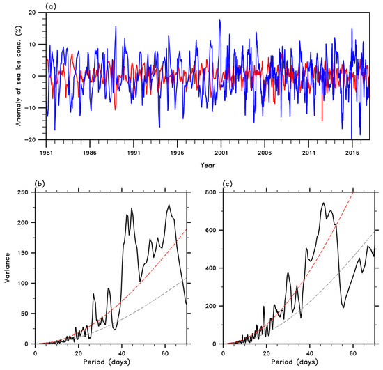
Figure 1.
(a) Wintertime (December–February) daily time series of sea ice concentration anomalies in the Bering Sea (red) and the Sea of Okhotsk (blue) from 1981 to 2017. Hereafter, 1981 denotes the December–January–February (DJF) of 1981 from 1 December 1981 to last day of February 1982 as an example. (b) and (c) indicate the power spectrum (black solid), red noise curve (gray dashed), and 95% confidence bounds (red dashed) for the Bering Sea and the Sea of Okhotsk, respectively.
The power spectra indicate that the intraseasonal variabilities are dominant in both seas (Figure 1b,c). Common significant peaks are found near 40–50 days, i.e., the characteristic timescale of the MJO, indicating that intraseasonal variabilities of SIC for both basins are possibly in accordance with the MJO. However, the separate outstanding peak at 60–65 days in the Bering Sea SIC time series is notable. Assuming that it has a physical reason, some speculations can be suggested as follows: (1) there could be the MJO-induced propagating waves with slower velocity that only cross the Bering Sea [24,25]; (2) the interaction with the other low-frequency oscillations (e.g., the North Pacific Oscillation (NPO), ENSO, etc.) could generate the lengthened timescale of intraseasonal variability [26]; and (3) the slower oceanic phenomenon (e.g., ocean eddies) in the Bering Sea could be responsible for the spectral peak [27]. Because thorough dynamical analyses are needed to prove this, we leave these topics for a future study.
In order to relate the sea ice variability in the Pacific sector of the Arctic with the large-scale conditions associated with the MJO, we conducted a composite analysis with respect to each MJO phase. The occurrence of each MJO phase was defined when the amplitude for the phase exceeds its standard deviation from the average. The first day of occurrence of each peak phase was set by a lag 0 day. According to Figure 2, the opposite ∆SIC is clearly shown between the Bering Sea and the Sea of Okhotsk in most of the phases. In the Bering Sea (the Sea of Okhotsk), a positive ∆SIC is predominant in phases 2–4 (phases 6 and 7), while a negative ∆SIC is evident in phases 6 and 7 (phases 2–4).
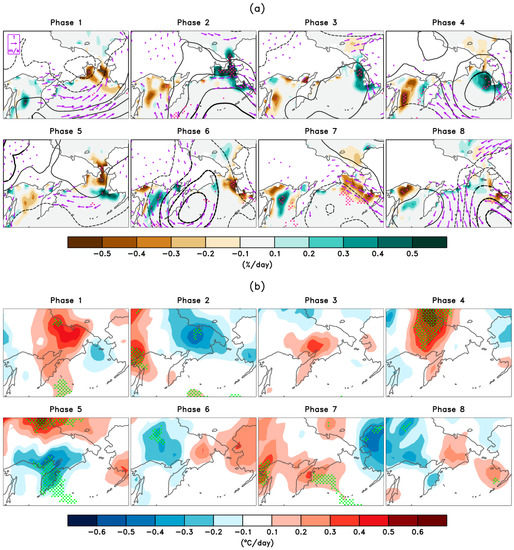
Figure 2.
Seven-day mean anomaly composites of (a) daily change in sea ice concentration (ΔSIC, shading), sea level pressure (SLP, contour), and 10 m winds (arrows), and (b) ΔT2m from day 4 to 10 after each Madden–Julian Oscillation (MJO) phase peak. The sea level pressure contour interval is 1 hPa from ±1 hPa, and the dashed lines represent the negative anomaly. The composites over the dotted or bold-lined regions are statistically significant at the 90% confidence level based on a Student’s t-test. Ten-meter wind anomalies are only plotted at statistically significant levels.
The dipole pattern of ∆SIC between the Bering Sea and the Sea of Okhotsk in each phase seems to be largely attributed to 10 m wind fields. In phases 2–4, anomalous southerly/southeasterly and northwesterly winds dominate the Sea of Okhotsk and the Bering Sea, respectively (Figure 2a). The northeastward wind-driven transport due to southerly/southeasterly winds could make the sea ice pull back to north shore of the Sea of Okhotsk, resulting in a sea ice reduction (Figure 3). In the Bering Sea, the increasing region of ∆SIC moves southward more gradually from phases 2 to 4. In phase 2, ∆SIC increases thermodynamically in relation to the cold advection due to northwesterly winds (Figure 2b). In addition, the convergence of sea ice motion in the Bering Strait could explain the increasing sea ice therein, although the sea ice motion is not easily attributable to wind vectors. For phases 3 and 4, however, it is clear that the southward wind-driven transport due to northwesterly winds likely spreads out sea ice, causing a sea ice increase (Figure 3). Meanwhile, except for the Bering Sea in phase 2, there are no noticeable air temperature changes over the two ocean basins during phases 2–4 (Figure 2b). Hence, sea ice changes seem to be more dominantly controlled by the dynamic process in the both ocean basins.
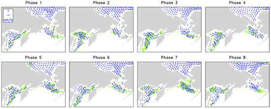
Figure 3.
Seven-day mean anomaly composites of sea ice motion from day 4 to 10 after each MJO phase peak. The composites over the green shaded regions are statistically significant at the 90% confidence level based on a Student’s t-test.In phases 6 and 7, anomalous northeasterly and southeasterly winds prevail in the Sea of Okhotsk and the Bering Sea, respectively (Figure 2a). Similarly, the southwestward wind-driven transport due to northeasterly wind extends sea ice in the Sea of Okhotsk (Figure 3). The northwestward wind-driven transport, due to southeasterly winds, leads sea ice to be contracted to the north so that sea ice retreats in the basin (Figure 3). Air temperature is not the main factor in the SIC variations in phases 6 and 7, although warm advection may affect the decrease in SIC in the Bering Sea in phase 6. According to our results, the dipole pattern in sea ice between the Bering Sea and the Sea of Okhotsk is evident in phases 2–4 and phases 6–7. Because of their similarity of mechanism to control sea ice change, i.e., wind-driven transport, we will hereafter focus more on phases 3 and 7 of the MJO for a simpler approach. In addition, the MJO-induced teleconnection patterns are not so different within each phase group, i.e., phases 2–4 and phases 6–7 (not shown).
The 10 m wind field strongly depends on the SLP pattern over the North Pacific. In SLP composites, the eastward tilted dipole patterns are evident between the North Pacific and Alaska in both phases 3 and 7 (Figure 4a). In phase 3, an anomalous high and low are located in the North Pacific and Alaska, respectively. The opposite is true for phase 7. These SLP patterns exactly correspond to the 10 m wind vectors shown in Figure 2. Since we hypothesized herein that the SLP patterns are attributable to the planetary Rossby waves being stimulated by MJO-related tropical convection, the 300 hPa eddy geopotential height fields were also investigated. As can be seen in Figure 4b, in the upper-level troposphere, the planetary Rossby waves are clearly displayed. Enhanced tropical convection over the Indian Ocean (in phase 3) causes the negative PNA-like pattern, while that over the central Pacific (in phase 7) creates a positive PNA-like pattern. In fact, several studies have suggested that active (inactive) convection in the Indian Ocean and the western Pacific is likely related to the negative (positive) PNA pattern [14,23]. According to our results, the upper-level eddy geopotential height nearly corresponds to the SLP pattern. These strong barotropic structures in both phases strongly support the idea that the SLP pattern is modulated by the planetary Rossby waves stimulated by the MJO-related tropical heating.
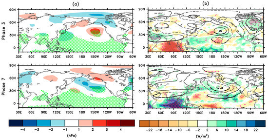
Figure 4.
Seven-day mean anomaly composites of (a) SLP and (b) outgoing longwave radiation (OLR) (shading) and a 300 hPa eddy geopotential height (contour) for MJO phases 3 and 7. Composite averages were taken from each MJO phase peak date for OLR and day 4 to 10 after each MJO phase peak for others. The interval of the 300 hPa geopotential height anomaly is 20 m from ±10 m, and the dashed line represents the negative anomaly. The composites over the dotted or bold-lined regions are statistically significant at the 90% confidence level based on a Student’s t-test.
To further verify the possible relation between sea ice and the MJO found in this study, representative cases of MJO phases 3 and 7 were selected when the amplitude of the RMM index was larger than two times the standard deviation from its mean (Figure 5). The chosen cases for phases 3 and 7 are 6 February 1985 (Case 1) and 1 January 1993 (Case 2), respectively. In Case 1, the negative PNA-like pattern gradually develops from lag 0 to lag +9 days after enhanced tropical convection in the Indian Ocean. A positive ∆SIC in the Bering Sea prevails throughout all the lag days, while a negative ∆SIC in the Sea of Okhotsk is dramatically enhanced after the lag +6 day. The latter is because anomalous southeasterly winds over the Sea of Okhotsk notably form after the lag +6 day. In Case 2, the positive PNA-like pattern is shown the lag +6 day after the suppression of tropical convection in the Indian Ocean. In the Bering Sea, similar to Case 1, a negative ∆SIC prevails throughout all the lag days, whereas, in the Sea of Okhotsk, a positive ∆SIC becomes noticeable after the lag +6 day but the signal is weaker, compared with Case 1, due to weaker prevailing wind anomalies therein.
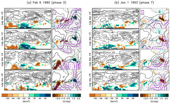
Figure 5.
Anomalies of the atmospheric variables and ∆SIC (a) on 6 February 1985 for phase 3 and (b) on 1 January 1993 for phase 7. Shading indicates the tropical OLR (∆SIC), and the contour is the eddy Z300 (SLP) in the left (right) panels. Arrows in the right panels are 10 m wind vectors with wind speeds above 5 m/s. The interval of the 300 hPa geopotential height (SLP) anomaly is 100 m (7 hPa) from ±50 m (±7 hPa), and dashed lines represent the negative anomaly.
4. Discussion and Conclusions
This study explored the MJO impact on wintertime SIC in the North Pacific sector, especially over the Bering Sea and the Sea of Okhotsk. Time series of intraseasonal SIC anomalies over the Bering Sea and the Sea of Okhotsk show a negative correlation, in agreement with the findings of previous works [28,29]. Moreover, both time series have significant power spectra of about 40–50 days, representing intraseasonal variations relevant to the characteristic MJO timescale. Intraseasonal variability of SIC accounts for up to 38% and 33% of the total variation over the Bering Sea and the Sea of Okhotsk, respectively. Given that the variations of SIC in the two seas are well synchronous with the evolution of the MJO, these amounts of explained variance may have implications on real SIC predictions using the MJO phase [30].
Figure 6 schematically summarizes the North Pacific sea ice response to the intraseasonal dynamical processes associated with the two core phases of the MJO (i.e., phases 3 and 7). At phase 3 of the MJO, enhanced convection over the tropical Indian Ocean remotely induces a wave train toward the North Pacific Ocean, forming a negative PNA-like pattern approximately one week after its peak date (Figure 6a). During this period, northwesterly (southeasterly) winds prevail, and the ∆SIC anomalies are positive (negative) in the Bering Sea (the Sea of Okhotsk) resulting in the SIC increase (decrease) via wind-driven ice drift. Meanwhile, suppressed convection over the Indian Ocean, representing the MJO phase 7, leads to a positive PNA-like pattern approximately one after its peak date (Figure 6b). This is responsible for southeasterly (northeasterly) winds over the Bering Strait (the Sea of Okhotsk), leading to the decrease (increase) in ∆SIC through wind-driven ice drift.
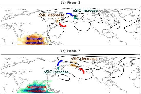
Figure 6.
Schematics of the MJO impacts on the atmospheric circulation and sea ice in the North Pacific for (a) phase 3 and (b) phase 7. The black solid lines and dashed circles denote anticyclonic and cyclonic circulation anomalies, respectively. The curly thick blue (red) arrows denote the wind anomalies with a northerly (southerly) component, and green (brown) shadings at high latitudes indicate an increase (a decrease) of SIC.
Our study is advanced from [12] in the following two aspects. Differently to [12], we considered the time lag of the influence of the MJO on the North Pacific teleconnection and brought the dipole sea ice modulation by the MJO over the North Pacific into focus. Taking the time lag into consideration, the intraseasonal SIC changes at the peak phases (i.e., 3 and 7) seem to be more dependent on wind-driven sea ice drift rather than temperature anomalies, because there is no promoting effect on the significant changes in ∆SIC by temperature anomalies in phases 3 and 7. Yet, as in [12], the temperature anomalies still seem to affect phases 2 and 6.
There are some crucial aspects which were not investigated in detail here. In the mid- and high-latitudes, the synoptic eddies, such as the locations, intensities, and tracks of the North Pacific storms also play a part in sustaining the low-frequency variability. In phase 3 (7), for example, an anomalous anticyclone (cyclone) in the Bering Sea implies less or weaker (more or stronger) storm activity, which co-occurs with the expansion (shrinking) of sea ice area in the region. This situation is very similar to the explanation of [31], where the authors noted that the sea ice extent in the Bering Sea is linked to wintertime storm track location on an interannual timescale. From a dynamical perspective, the storm activity is tightly linked to the low-frequency variability through the synoptic eddy feedback [32]. By nature, the synoptic eddy feedback sustains the low-frequency variabilities, such as the PNA, NPO, and AO/NAO, all of which are significantly modulated by the MJO in the tropics [16,23,33,34]. Therefore, further investigation on the role of synoptic storms in SIC changes under different MJO phases is necessary for the following study.
Author Contributions
Conceptualization, J.-H.K. and D.-S.R.P.; Methodology, J.-Y.H. and D.-S.R.P.; Formal Analysis, J.-Y.H.; Investigation, J.-Y.H., J.-H.K. and D.-S.R.P.; Writing—Original Draft, J.-Y.H.; Writing—Review and Editing, J.-H.K. and D.-S.R.P.; Visualization, J.-Y.H.; Supervision, J.-H.K. and D.-S.R.P.; Project Administration, J.-H.K.; Funding Acquisition, J.-H.K. All authors have read and agreed to the published version of the manuscript.
Funding
This study was funded by the Korea Polar Research Institute (KOPRI) project, entitled ‘Earth System Model-based Korea Polar Prediction System (KPOPS-Earth) Development and Its Application to the High-impact Weather Events originated from the Changing Arctic Ocean and Sea Ice’ (KOPRI, PE20090) and by the Ministry of Oceans and Fisheries, Korea project, entitled ‘Investigation and Prediction System Development of Marine Heatwave around the Korean Peninsula originated from the Sub-Arctic and Western Pacific’ (20190344).
Acknowledgments
The authors are grateful to the editor for the efficient handling of all processes and also thank the two anonymous reviewers for their suggestions and comments.
Conflicts of Interest
The authors declare no conflict of interest.
References
- Kim, K.-Y.; Kim, J.-Y.; Kim, J.; Yeo, S.; Na, H.; Hamlington, B.D.; Leben, R.R. Vertical feedback mechanism of winter Arctic amplification and sea ice loss. Sic. Rep. 2019, 9, 1184. [Google Scholar] [CrossRef] [PubMed]
- Screen, J.A.; Simmonds, I. Increasing fall-winter energy loss from the Arctic Ocean and its role in Arctic temperature amplification. Geophys. Res. Lett. 2010, 37, L16707. [Google Scholar] [CrossRef]
- Shimada, K.; Kamoshida, T.; Itoh, M.; Nishino, S.; Carmack, E.; McLaughlin, F.; Zimmermann, S.; Proshutinsky, A. Pacific Ocean inflow: Influence on catastrophic reduction of sea ice cover in the Arctic Ocean. Geophys. Res. Lett. 2006, 33, L08605. [Google Scholar] [CrossRef]
- Spielhagen, R.F.; Werner, K.; Sørensen, S.A.; Zamelczyk, K.; Kandiano, E.; Budeus, G.; Husum, K.; Marchitto, T.M.; Hald, M. Enhanced modern heat transfer to the Arctic by warm Atlantic water. Science 2011, 331, 450–453. [Google Scholar] [CrossRef] [PubMed]
- Fang, Z.; Wallace, J.M. Arctic sea ice variability on a timescale of weeks and its relation to atmospheric forcing. J. Clim. 1994, 7, 1897–1914. [Google Scholar] [CrossRef]
- Deser, C.; Walsh, J.E.; Timlin, M.S. Arctic sea ice variability in the context of recent atmospheric circulation trends. J. Clim. 2000, 13, 617–633. [Google Scholar] [CrossRef]
- Rigor, I.G.; Wallace, J.M.; Colony, R.L. Response of sea ice to the Arctic Oscillation. J. Clim. 2002, 15, 2648–2663. [Google Scholar] [CrossRef]
- Lee, S. A theory for polar amplification from a general circulation perspective. Asia–Pac. J. Atmos. Sci. 2014, 50, 31–43. [Google Scholar] [CrossRef]
- Ding, Q.; Wallace, J.M.; Battisti, D.S.; Steig, E.J.; Gallant, A.J.E.; Kim, H.-J.; Geng, L. Tropical forcing of the recent rapid Arctic warming in northeastern Canada and Greenland. Nature 2014, 509, 209–212. [Google Scholar] [CrossRef]
- Madden, R.A.; Julian, P.R. Detection of a 40–50 day oscillation in the zonal wind in the tropical Pacific. J. Atmos. Sci. 1971, 28, 702–708. [Google Scholar] [CrossRef]
- Yoo, C.; Lee, S.; Feldstein, S.B. Mechanisms of Arctic surface air temperature change in response to the Madden–Julian oscillation. J. Clim. 2012, 25, 5777–5790. [Google Scholar] [CrossRef]
- Henderson, G.R.; Barrett, B.S.; Lafleur, D.M. Arctic sea ice and the Madden–Julian Oscillation (MJO). Clim. Dyn. 2014, 43, 2185–2196. [Google Scholar] [CrossRef]
- Yoo, C.; Lee, S.; Feldstein, S.B. Arctic response to an MJO-like tropical heating in an idealized GCM. J. Atmos. Sci. 2012, 69, 2379–2393. [Google Scholar] [CrossRef]
- Mori, M.; Watanabe, M. The growth and triggering mechanisms of the PNA: A MJO-PNA coherence. J. Meteorol. Soc. Jpn. 2008, 86, 213–236. [Google Scholar] [CrossRef]
- Seo, K.-H.; Son, S.-W. The global atmospheric circulation response to tropical diabatic heating associated with the Madden–Julian oscillation during northern winter. J. Atmos. Sci. 2012, 69, 79–96. [Google Scholar] [CrossRef]
- Henderson, S.A.; Maloney, E.D.; Son, S.-W. Madden–Julian oscillation Pacific teleconnections: The impact of the basic state and MJO representation in general circulation models. J. Clim. 2017, 30, 4567–4587. [Google Scholar] [CrossRef]
- Ukita, J.; Honda, M.; Nakamura, H.; Tachibana, Y.; Cavalieri, D.J.; Parkinson, C.L.; Koide, H.; Yamamoto, K. Northern Hemisphere sea ice variability: Lag structure and its implications. Tellus A 2007, 59, 261–272. [Google Scholar] [CrossRef]
- Dee, D.P.; Uppala, S.M.; Simmons, A.J.; Berrisford, P.; Poli, P.; Kobayashi, S.; Andrae, U.; Balmaseda, M.A.; Balsamo, G.; Bauer, P.; et al. The ERA-Interim reanalysis: Configuration and performance of the data assimilation system. Q. J. R. Meteorol. Soc. 2011, 137, 553–597. [Google Scholar] [CrossRef]
- Liebmann, B.; Smith, C.A. Description of a complete (interpolated) outgoing longwave radiation dataset. Bull. Am. Meteorol. Soc. 1996, 77, 1275–1277. [Google Scholar]
- Tschudi, M.; Meier, W.N.; Stewart, J.S.; Fowler, C.; Maslanik, J. Polar Pathfinder Daily 25 km EASE-grid Sea Ice Motion Vectors, Version 4; NASA National Snow and Ice Data Center Distributed Active Archive Center: Boulder, CO, USA, 2019. [Google Scholar] [CrossRef]
- Wheeler, M.C.; Hendon, H.H. An all-season real-time multivariate MJO index: Development of an index for monitoring and prediction. Mon. Weather Rev. 2004, 132, 1917–1932. [Google Scholar] [CrossRef]
- Lee, M.-H.; Kim, J.-H. The role of synoptic cyclones for the formation of Arctic summer circulation patterns as clustered by Self-Organizing Maps. Atmosphere 2019, 10, 474. [Google Scholar] [CrossRef]
- Seo, K.-H.; Lee, H.-J. Mechanisms for a PNA-like teleconnection pattern in response to the MJO. J. Atmos. Sci. 2017, 74, 1767–1781. [Google Scholar] [CrossRef]
- Seo, K.-H.; Lee, H.-J.; Frierson, D.M.W. Unraveling the teleconnection mechanisms that induce wintertime temperature anomalies over the Northern Hemisphere continents in response to the MJO. J. Atmos. Sci. 2016, 73, 3557–3571. [Google Scholar] [CrossRef]
- Lee, R.W.; Woolnough, S.J.; Charlton-Perez, A.J.; Vitart, F. ENSO modulation of MJO teleconnections to the North Atlantic and Europe. Geophys. Res. Lett. stage of publication (in press). [CrossRef]
- Moon, J.-Y.; Wang, B.; Ha, K.-J. ENSO regulation of MJO teleconnection. Clim. Dyn. 2011, 37, 1133–1149. [Google Scholar] [CrossRef]
- Dong, C.; Gao, X.; Zhang, Y.; Yang, J.; Zhang, H.; Chao, Y. Multiple-scale variations of sea ice and ocean circulation in the Bering Sea using remote sensing observations and numerical modeling. Remote Sens. 2019, 11, 1484. [Google Scholar] [CrossRef]
- Liu, J.; Zhang, Z.; Horton, R.M.; Wang, C.; Ren, X. Variability of north Pacific sea ice and East Asia–north Pacific winter climate. J. Clim. 2007, 20, 1991–2001. [Google Scholar] [CrossRef]
- Budikova, D. Role of Arctic sea ice in global atmospheric circulation: A review. Glob. Planet. Chang. 2009, 68, 149–163. [Google Scholar] [CrossRef]
- Lee, H.-J.; Seo, K.-H. Impact of the Madden-Julian oscillation on Antarctic sea ice and its dynamical mechanism. Sic. Rep. 2019, 9, 10761. [Google Scholar] [CrossRef]
- Overland, J.E.; Pease, C.H. Cyclone climatology of the Bering Sea and its relation to sea ice extent. Mon. Weather Rev. 1982, 110, 5–13. [Google Scholar] [CrossRef]
- Kug, J.-S.; Jin, F.-F. Left-hand rule for synoptic eddy feedback on low-frequency flow. Geophys. Res. Lett. 2009, 36, L05709. [Google Scholar] [CrossRef]
- Zhou, S.; Miller, A.J. The interaction of the Madden–Julian Oscillation and the Arctic Oscillation. J. Clim. 2005, 18, 143–159. [Google Scholar] [CrossRef]
- Lin, H.; Brunet, G.; Derome, J. An observed connection between the North Atlantic Oscillation and the Madden-Julian Oscillation. J. Clim. 2009, 22, 364–380. [Google Scholar] [CrossRef]
© 2019 by the authors. Licensee MDPI, Basel, Switzerland. This article is an open access article distributed under the terms and conditions of the Creative Commons Attribution (CC BY) license (http://creativecommons.org/licenses/by/4.0/).