Diurnal Variations of Surface and Air Temperatures on the Urban Streets in Seoul, Korea: An Observational Analysis during BBMEX Campaign

 , ,
, ,
Abstract
1. Introduction
2. Data and Methods
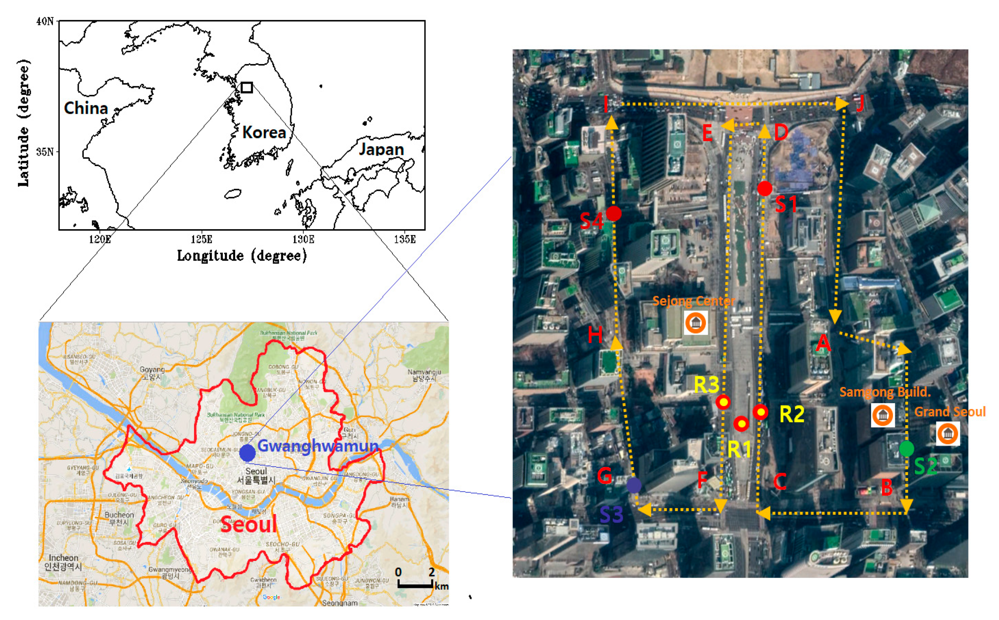
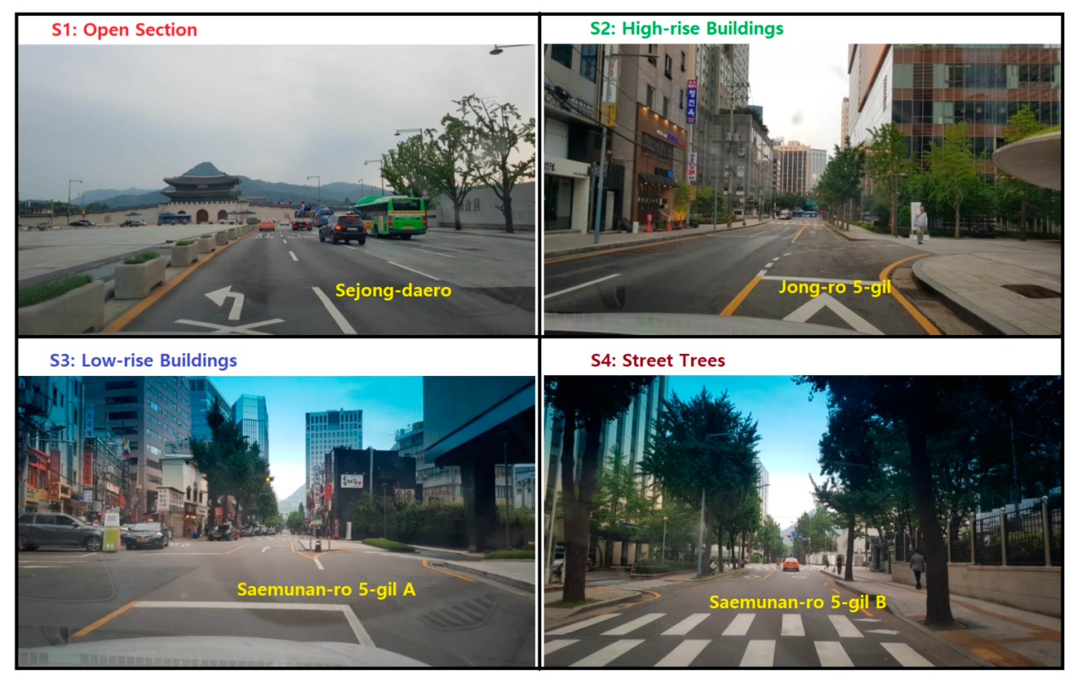
2.1. Study Area
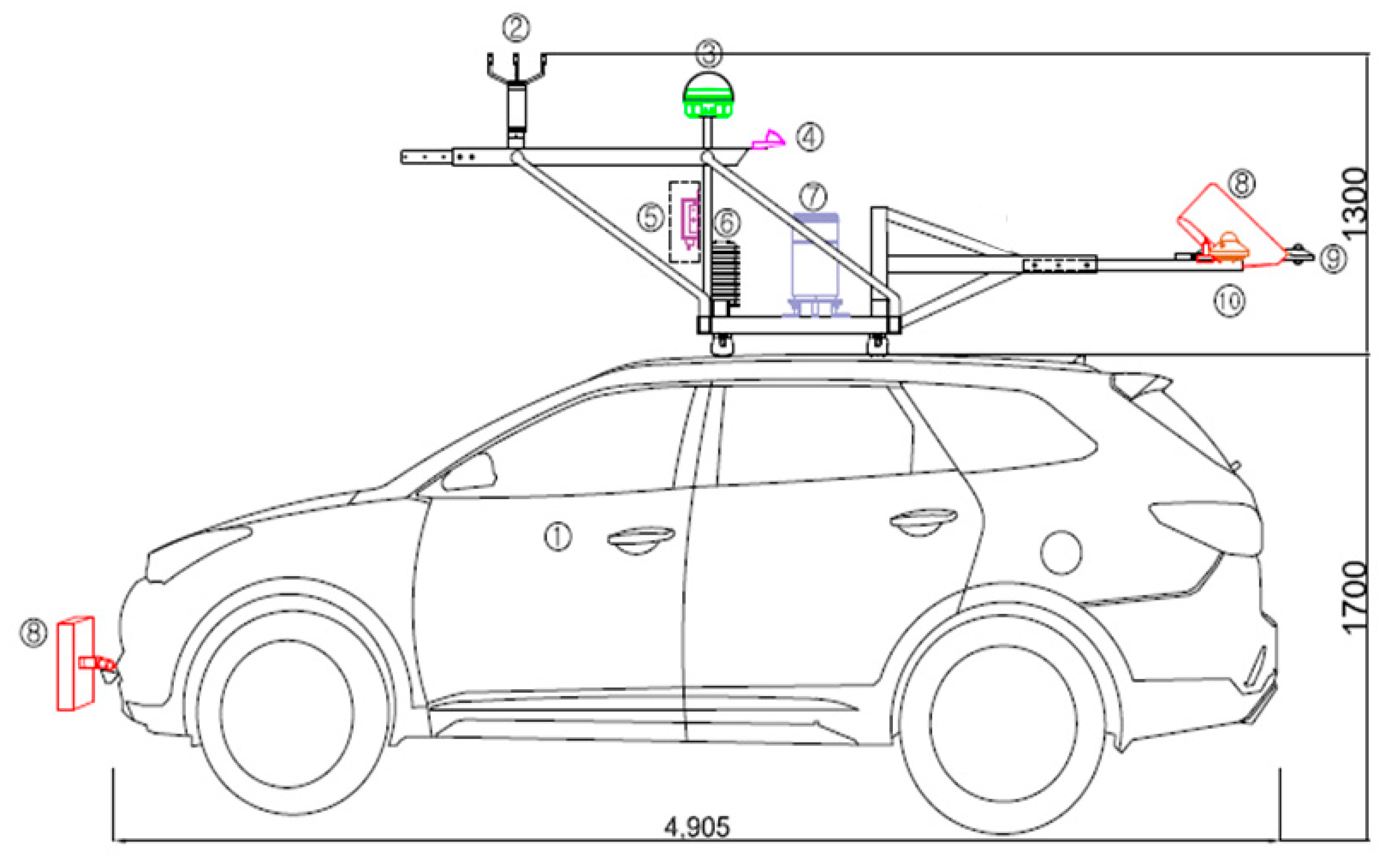
2.2. MOVE Dataset
2.3. BBMEX and Environmental Parameters
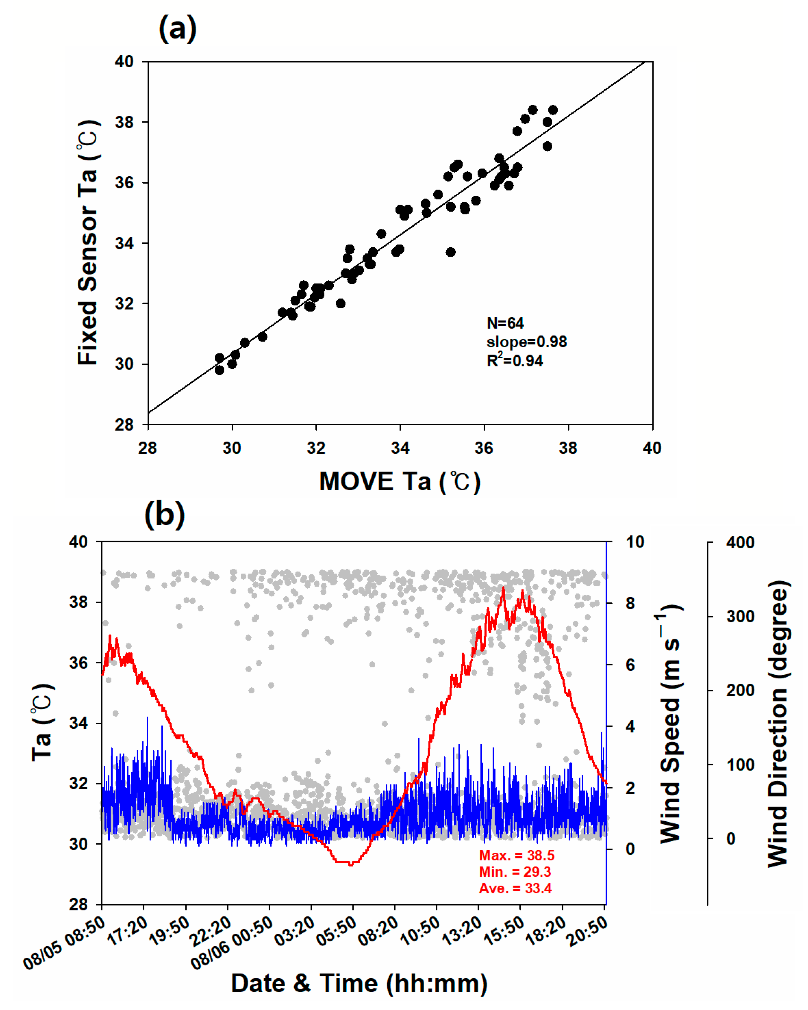
3. Data Validation
4. Results
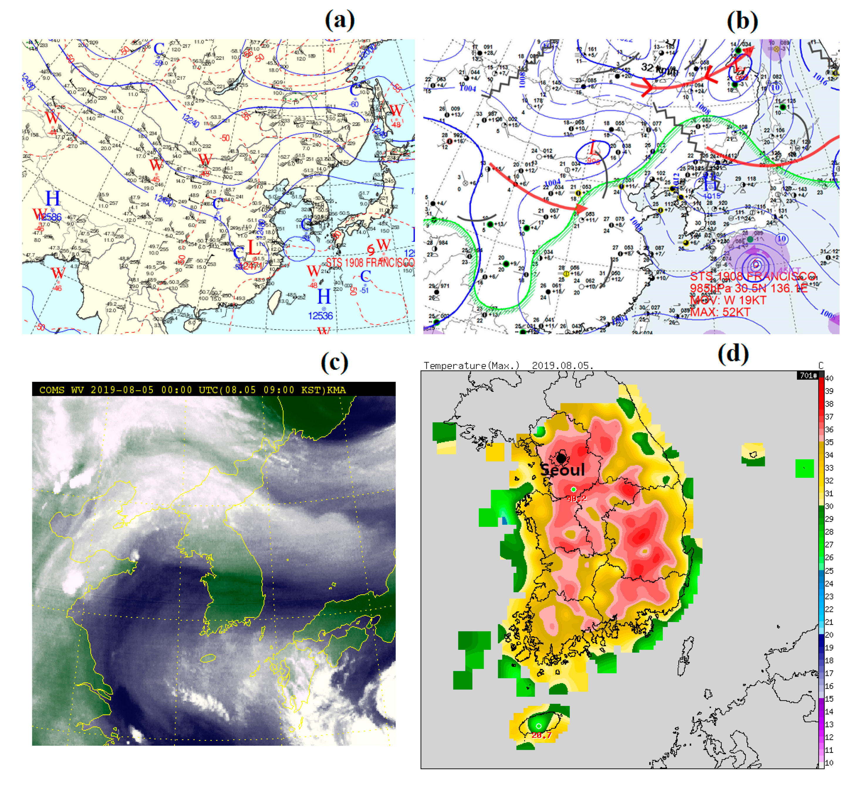
4.1. Synoptic Analysis
4.2. RST Distributions over the Study Area
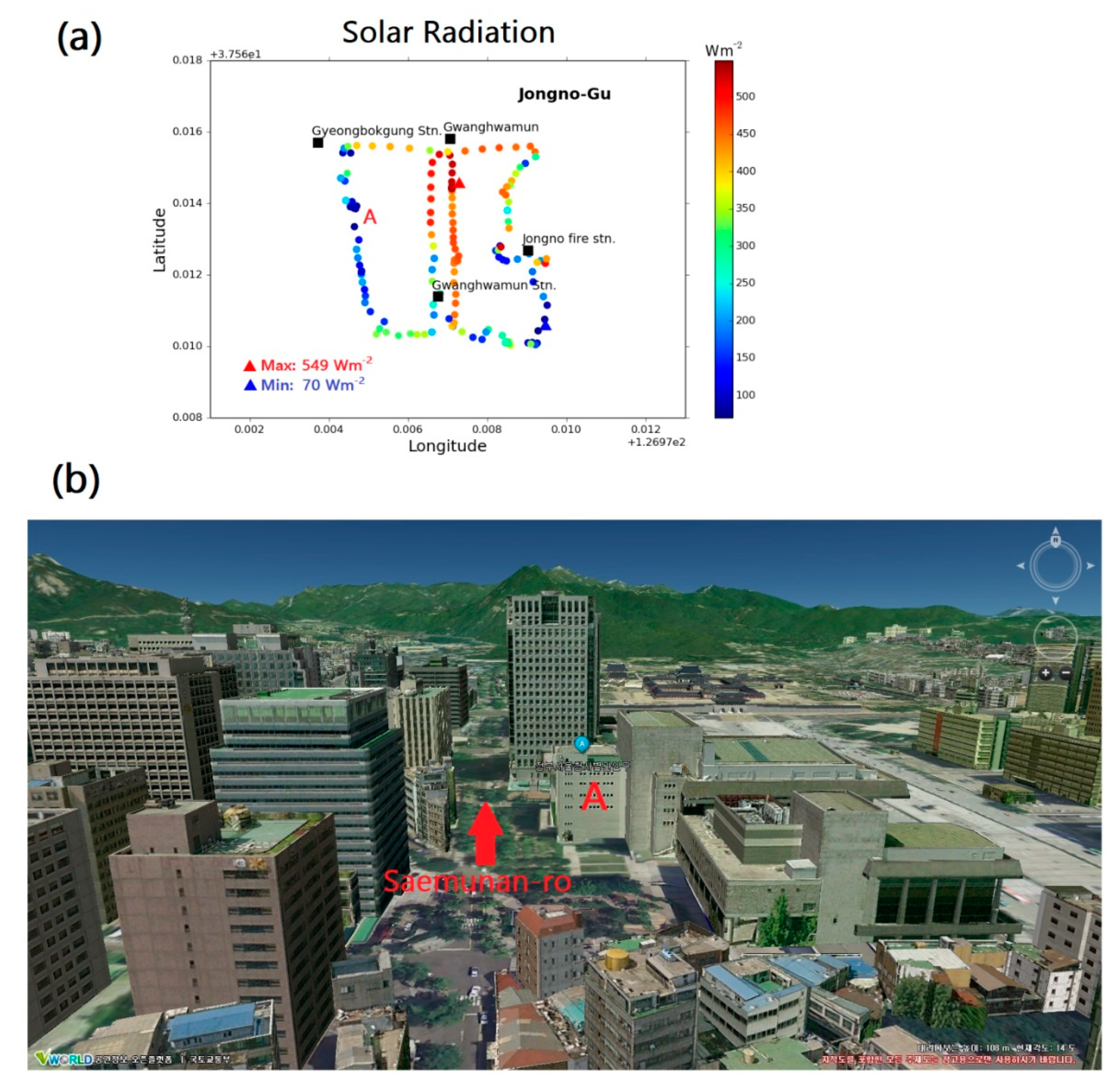
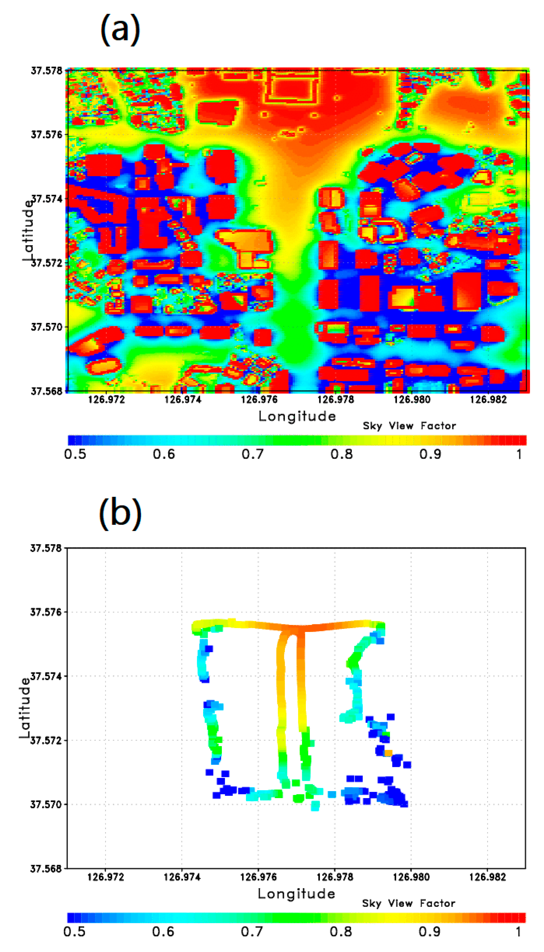
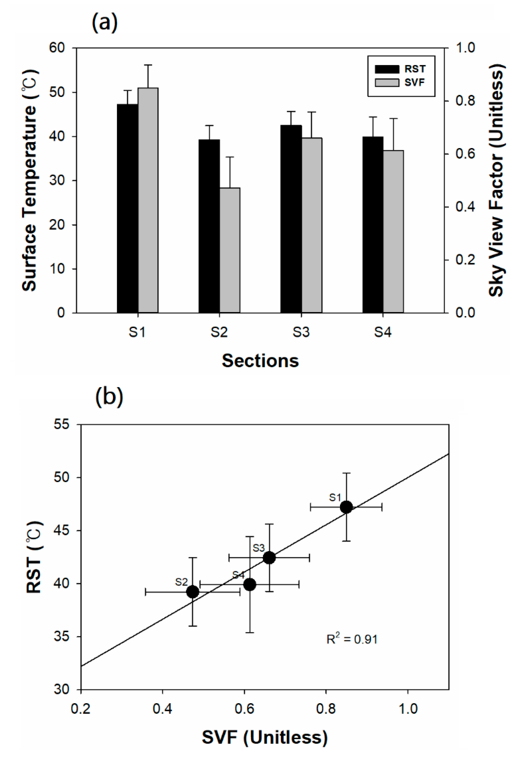
4.3. Comparison of the Factors Influencing RST
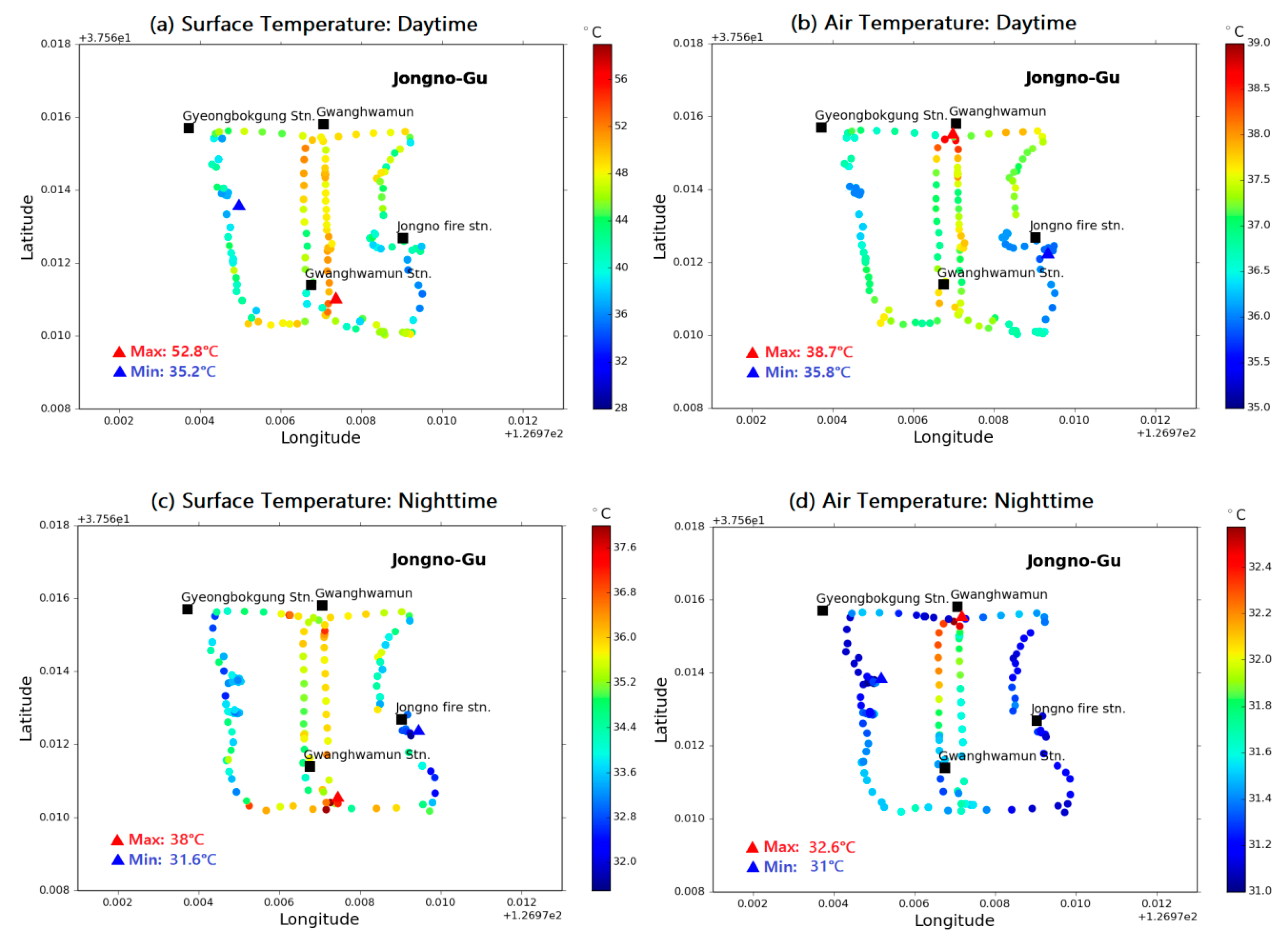
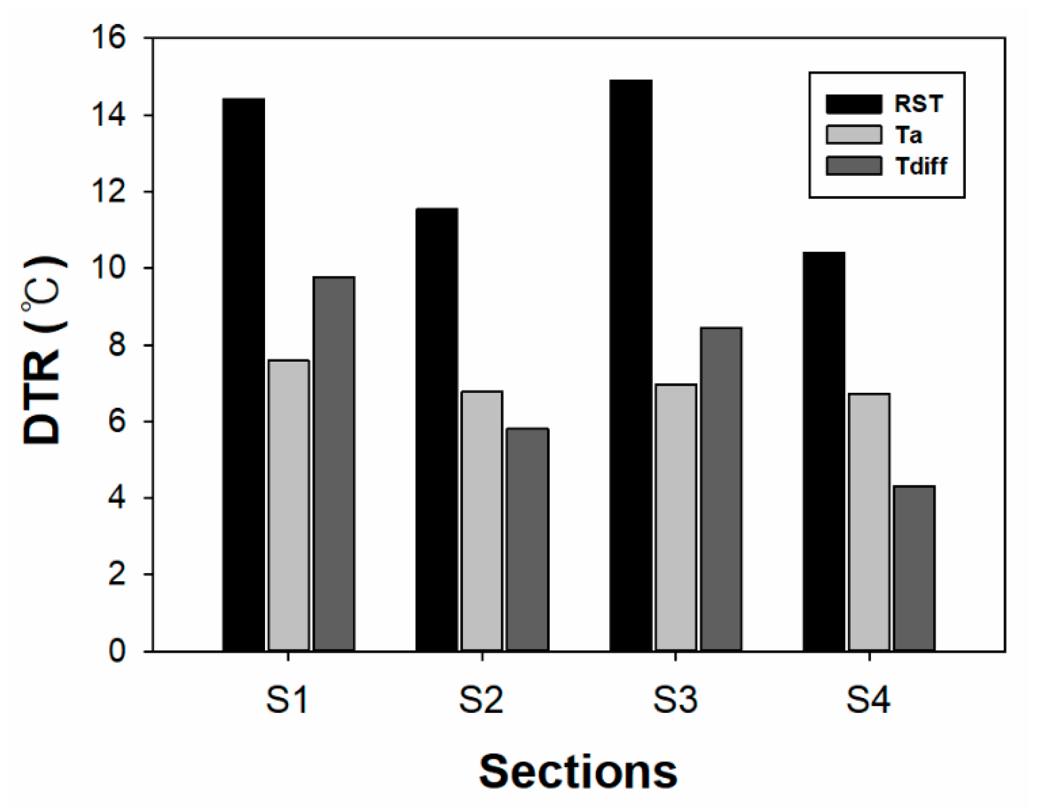
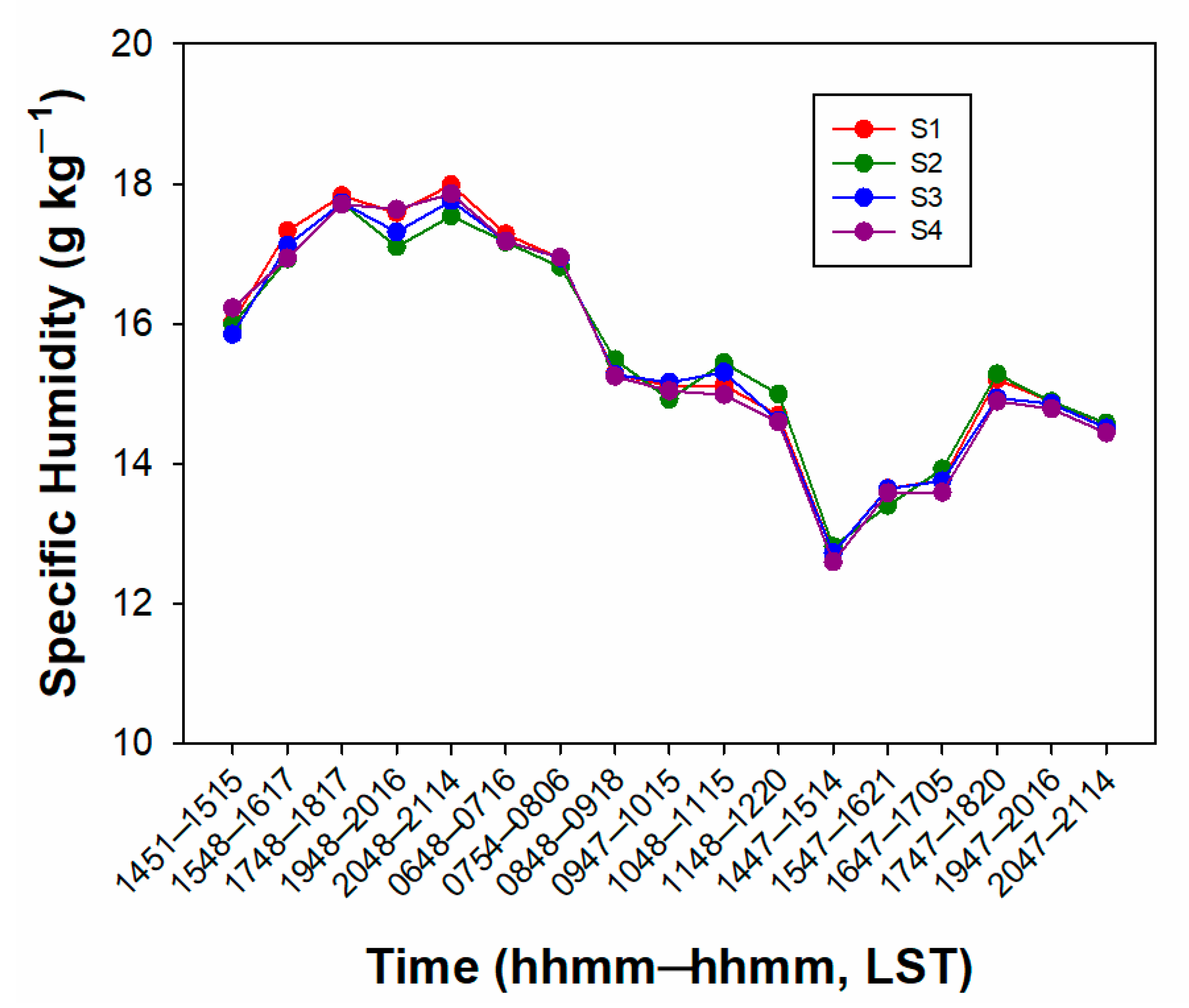
4.4. Diurnal Variations
5. Discussion
6. Conclusions
Author Contributions
Funding
Acknowledgments
Conflicts of Interest
References
- Barnett, A.G. Temperature and cardiovascular deaths in the US elderly: Changes over time. Epidemiology 2007, 18, 369–372. [Google Scholar] [CrossRef] [PubMed]
- Schubert, S.D.; Wang, H.; Koster, R.D.; Suarez, M.J. Northern Eurasian heat waves and droughts. J. Clim. 2014, 27, 3169–3207. [Google Scholar] [CrossRef]
- Kim, D.-W.; Deo, R.C.; Lee, J.-S.; Yeom, J.-M. Mapping heatwave vulnerability in Korea. Nat. Hazards 2017, 89, 35–55. [Google Scholar] [CrossRef]
- McCarthy, M.P.; Best, M.J.; Betts, R.A. Climate change in cities due to global warming and urban effects. Geophys. Res. Lett. 2010, 37, L09705. [Google Scholar] [CrossRef]
- Papanastasiou, D.K.; Melas, D.; Bartzanas, T.; Kittas, C. Temperature, comfort and pollution levels during heat waves and the role of sea breeze. Int. J. Biometeorol. 2010, 54, 307–317. [Google Scholar] [CrossRef] [PubMed]
- Ha, K.J.; Yun, K.S. Climate change effects on tropical night days in Seoul, Korea. Theor. Appl. Climatol. 2012, 109, 191–203. [Google Scholar] [CrossRef]
- Campbell, F.C. Elements of Metallurgy and Engineering Alloys; OCLC 608624525; ASM International: Materials Park, OH, USA, 2008; ISBN 9780871708670. [Google Scholar]
- Synnefa, A.; Karlessi, T.; Gaitani, N. Experimental testing of cool colored thin layer asphalt and estimation of its potential to improve the urban microclimate. Build. Environ. 2010, 46, 38–44. [Google Scholar] [CrossRef]
- Kim, Y.-J.; Kim, B.-J.; Shin, Y.-S.; Kim, H.-W.; Kim, G.-T.; Kim, S.-J. A case study of environmental characteristics on urban road-surface and air temperatures during heat-wave days in Seoul. Atmos. Ocean. Sci. Lett. 2019, 12, 261–269. [Google Scholar] [CrossRef]
- Bae, W.K.; Yoon, K.H. A design guideline of the apartment house complex for mitigation of heat island effect–For the planning agenda constructed and elected in 2005–2010. J. Archit. Inst. Korean Plan. 2012, 13, 47–60. [Google Scholar]
- Chung, M.H.; Park, J.C. Development of PCM cool roof system to control urban heat island considering temperate climatic conditions. Energy Build. 2016, 116, 248–341. [Google Scholar] [CrossRef]
- Jeong, J.; Chung, M.H. The planning of micro-climate control by complex types. Int. J. Korea Inst. Ecol. Archit. Environ. 2017, 17, 49–54. [Google Scholar] [CrossRef]
- Yamazaki, F.; Murakoshi, A.; Sekiya, N. Observation of urban heat island using airborne thermal sensors. In Proceedings of the 2009 Joint Urban Remote Sensing Event, Shanghai, China, 20–22 May 2009. [Google Scholar]
- Yoon, J. Field measurement recorded in the urban thermal environment of a medium-size city in autumn and winter. J. Archit. Inst. Korea Plan. 2009, 25, 453–460. [Google Scholar]
- Lee, S.; Moon, H.; Choi, Y.; Yoon, D.K. Analyzing thermal characteristics of urban streets using a thermal imaging camera: A case study on commercial streets in Seoul, Korea. Sustainability 2018, 10, 519. [Google Scholar] [CrossRef]
- Ibrahim, F. Urban land use land cover changes and their effect on land surface temperature: Case study using Dohuk City in the Kurdistan Region of Iraq. Climate 2017, 5, 13. [Google Scholar] [CrossRef]
- Zhang, X.; Estoque, R.C.; Murayama, Y. An urban heat island study in Nanchang City, China based on land surface temperature and social-ecological variables. Sustain. Cities Soc. 2017, 32, 557–568. [Google Scholar] [CrossRef]
- Zhao, Z.-Q.; He, B.-J.; Li, L.-G.; Wang, H.-B.; Darko, A. Profile and concentric zonal analysis of relationships between land use/land cover and land surface temperature: Case study of Shenyang, China. Energy Build. 2017, 155, 282–295. [Google Scholar] [CrossRef]
- Yang, K.; Yu, Z.; Luo, Y.; Yang, Y.; Zhao, L.; Zhou, X. Spatial and temporal variations in the relationship between lake water surface temperatures and water quality–A case study of Dianchi Lake. Sci. Total Environ. 2018, 624, 859–871. [Google Scholar] [CrossRef]
- He, B.-J.; Zhao, Z.-Q.; Shen, L.-D.; Wang, H.-B.; Li, L.-G. An approach to examining performances of cool/hot sources in mitigating/enhancing land surface temperature under different temperature backgrounds based on landsat 8 image. Sustain. Cities Soc. 2019, 44, 416–427. [Google Scholar] [CrossRef]
- Shao, J.; Swanson, J.C.; Patterson, R.; Lister, P.J.; McDonald, A.N. Variation of winter road surface temperature due to topography and application of thermal mapping. Meteorol. Appl. 1997, 4, 131–137. [Google Scholar] [CrossRef]
- Bogren, J.; Gustavsson, T.; Karlsson, M.; Postgård, U. The impact of screening on road surface temperature. Meteorol. Appl. 2000, 7, 97–104. [Google Scholar] [CrossRef]
- Postgård, U.; Lindqvist, S. Air and road surface temperature variations during weather change. Meteorol. Appl. 2001, 8, 71–84. [Google Scholar] [CrossRef]
- Chao, J.; Zhang, J. Prediction model for asphalt pavement temperature in high-temperature season in Beijing. Adv. Civ. Eng. 2018, 1–11. [Google Scholar] [CrossRef]
- Dai, A.; Kevin, E.T.; Thomas, R.K. Effects of clouds, soil moisture, precipitation, and water vapor on diurnal temperature range. J. Clim. 1999, 12, 2451–2473. [Google Scholar] [CrossRef]
- Liu, W.; Feddema, J.; Hu, L.; Zung, A.; Brunsell, N. Seasonal and diurnal characteristics of land surface temperature and major explanatory factors in Harris Country, Texas. Sustainability 2017, 9, 2324. [Google Scholar] [CrossRef]
- Bilbao, J.; Román, R.; Miguel, A.D. Temporal and spatial variability in surface air temperature and diurnal temperature range in Spain over the period 1950–2011. Climate 2019, 7, 16. [Google Scholar] [CrossRef]
- Grimmond, S. Urbanization and global environmental change: Local effects of urban warming. Geogr. J. 2007, 173, 83–88. [Google Scholar] [CrossRef]
- Unger, J. Connection between urban heat island and sky view factor approximated by a software tool on a 3D urban database. Int. J. Environ. Pollut. 2008, 36, 59–80. [Google Scholar] [CrossRef]
- Ha, J.; Lee, S.; Park, C. Temporal effects of environmental characteristics on urban air temperature: The influence of the sky view factor. Sustainability 2016, 8, 895. [Google Scholar] [CrossRef]
- Solaimanian, M.; Kennedy, T.W. Predicting maximum pavement surface temperature using maximum air temperature and hourly solar radiation. Transp. Res. Rec. 1993, 1417, 1–11. [Google Scholar]
- Offerle, B.; Eliasson, I.; Grimmond, C.S.B. Surface heating in relation to air temperature, wind and turbulence in an urban street canyon. Bound. Layer Meteorol. 2007, 122, 273–292. [Google Scholar] [CrossRef]
- Park, M.-S.; Park, S.-H.; Chae, J.-H.; Choi, M.-H.; Song, Y.; Kang, M.; Roh, J.-W. High-resolution urban observation network for user-specific meteorological information service in the Seoul Metropolitan Area, South Korea. Atmos. Meas. Tech. 2017, 10, 1575–1594. [Google Scholar] [CrossRef]
- World Meteorological Organization. Guide to Meteorological Instruments and Methods of Observation; WMO: Geneva, Switzerland, 1996; Available online: http://hdl.handle.net/11329/83 (accessed on 29 November 2019).
- Kim, Y.-J.; Kim, S.-J.; Kim, G.-T.; Choi, B.-C.; Shim, J.-K.; Kim, B.-G. Retrieval and validation of precipitable water vapor using GPS datasets of mobile observation vehicle on the eastern coast of Korea. Korean J. Remote Sens. 2016, 4, 365–382. [Google Scholar] [CrossRef]
- Chun, B.S.; Guldmann, J.M. Spatial statistical analysis and simulation of the urban heat island in high-density central cities. Landsc. Urban Plan. 2014, 125, 76–88. [Google Scholar] [CrossRef]
- Bernard, J.; Bocher, E.; Petit, G.; Palominos, S. Sky view factor calculation in urban context: Computational performance and accuracy analysis of two open and free GIS tools. Climate 2018, 6, 60. [Google Scholar] [CrossRef]
- Jee, J.-B.; Zo, I.-S.; Kim, B.-Y.; Lee, K.-T. An analysis of observational environments for solar radiation stations of Korea meteorological administration using the digital elevation model and solar radiation model. J. Korean Earth Sci. Soc. 2019, 40, 119–134, (In Korean with English abstract). [Google Scholar] [CrossRef]
- Bolton, D. The computation of equivalent potential temperature. Mon. Weather Rev. 1980, 108, 1046–1053. [Google Scholar] [CrossRef]
- He, B.-J.; Ding, L.; Prasad, D. Enhancing urban ventilation performance through the development of precinct ventilation zones: A case study based on the Greater Sydney, Australia. Sustain. Cities Soc. 2019, 47, 101472. [Google Scholar] [CrossRef]
- Lindberg, F.; Holmer, B.; Thorsson, S. SOLWEIG 1.0—Modeling spatial variations of 3D radiant fluxes and mean radiant temperature in complex urban settings. Int. J. Biometeorol. 2008, 52, 697–713. [Google Scholar] [CrossRef]
- Gál, T.; Lindberg, F.; Unger, J. Computing continuous sky view factors using 3D urban raster and vector databases: Comparison and application to urban climate. Theor. Appl. Climatol. 2009, 95, 111–123. [Google Scholar] [CrossRef]
- Kastendeuch, P.P. A method to estimate sky view factors from digital elevation models. Int. J. Climatol. 2013, 33, 1574–1578. [Google Scholar] [CrossRef]
- Hämmerle, M.; Gál, T.; Unger, J.; Matzarakis, A. Comparison of models calculating the sky view factor used for urban climate investigations. Theor. Appl. Climatol. 2011, 105, 521–527. [Google Scholar] [CrossRef]
- Jee, J.-B.; Yang, H.-J.; Lee, C.-Y.; Min, J.-S.; Kang, M.-S. Comparison of surface characteristics information retrievals and simulation of detailed temperature and wind field distributions using digital DSM and 3D camera image. In Proceedings of the Autumn Meeting of KMS 2019, Seoul, South Korea, 25–27 October 2019. [Google Scholar]
- Ramamurthy, P.; Jorge, G.; Luis, O.; Mark, A.; Fred, M. Impact of heatwave on a megacity: An observational analysis of New York City during July 2016. Environ. Res. Lett. 2017, 12, 054011. [Google Scholar] [CrossRef]
- Ramamurthy, P.; Bou-Zeid, E.; Wang, Z.; Smith, J.; Baek, M.; Welty, C.; Hom, J.; Saliendra, N. Influence of sub-facet heterogeneity and matrial properties on the urban surface energy budget. J. Appl. Meteorol. Climatol. 2014, 53, 2114–2129. [Google Scholar] [CrossRef]
- Li, D.; Bou-Zeid, E. Synergistic interactions between urban heat island and heat waves: The impact in cities is larger than the sum of its parts. Environ. Res. Lett. 2013, 52, 2051–2064. [Google Scholar] [CrossRef]
- Doulos, L.; Santamouris, M.; Livada, I. Passive cooling of outdoor urban spaces. The role of materials. Sol. Energy 2004, 77, 231–249. [Google Scholar] [CrossRef]
- McMichael, A.J.; Campbell-Lendrum, D.H.; Corvalán, C.F.; Ebi, K.L.; Githeko, A.K.; Scheraga, J.D.; Woodward, A. Climate Change and Human Health: Risks and Responses; World Health Organization: Geneva, Switzerland, 2003; ISBN 92-4-1-56248-X. [Google Scholar]
- Loughner, C.P.; Allen, D.J.; Zhang, D.-L.; Pickering, K.E.; Dickerson, R.R.; Landry, L. Roles of urban tree canopy and buildings in urban heat island effects: Parameterization and preliminary results. J. Appl. Meteorol. Clim. 2012, 51, 1775–1793. [Google Scholar] [CrossRef]
- Kwak, K.-H.; Lee, S.-H.; Seo, J.M.; Park, S.-B.; Baik, J.-J. Relationship between rooftop and on-road concentrations of traffic-related pollutants in a busy street canyon: Ambient wind effects. Environ. Pollut. 2016, 208, 185–197. [Google Scholar] [CrossRef]
- Kwak, K.-H.; Woo, S.H.; Kim, K.H.; Lee, S.-B.; Bae, G.-N.; Ma, Y.I.; Sunwoo, Y.; Baik, J.-J. On-road air quality associated with traffic composition and street-canyon ventilation: Mobile monitoring and CFD modeling. Atmosphere 2018, 9, 92. [Google Scholar] [CrossRef]
- Luo, Y.; Li, Q.; Yang, K.; Xie, W.; Zhou, X.; Shang, C.; Xu, Y.; Zhang, Y.; Zhang, C. Thermodynamic analysis of air-ground and water-ground energy exchange process in urban space at micro scale. Sci. Total Environ. 2019, 694, 133612. [Google Scholar] [CrossRef]
- Sailor, D.J. Simulated urban climate response to modifications in surface albedo and vegetative cover. J. Appl. Meteorol. 1995, 34, 1694–1704. [Google Scholar] [CrossRef]
- Pomerantz, M.; Pon, B.; Akbari, H.; Chang, S.C. The Effect of Pavements’ Temperatures on Air Temperatures in Large Cities; LBNL-43442; Lawrence Berkeley National Laboratory: Berkeley, CA, USA, 2000. [Google Scholar]
- Guan, K.K. Surface and ambient air temperatures associated with different ground materials: A case study at the university of California, Berkeley. Environ. Sci. 2011, 196, 1–14. [Google Scholar]
- Honjo, T.; Lin, T.-P.; Seo, Y. Skyview factor measurement by using a spherical camera. J. Agric. Meteorol. 2019, 75, 59–66. [Google Scholar] [CrossRef]


| Road Sections | Road Names | Remarks |
|---|---|---|
| A→B | Jong-ro 5-gil | - |
| B→C | Jong-ro | - |
| C→D | Sejong-daero | - |
| D→E | Sajik-ro | Traffic light (U-turn) |
| E→F | Sejong-daero | - |
| F→G | Saemunan-ro | - |
| G→H | Saemunan-ro 5-gil | - |
| H→I | Saemunan-ro 5-gil | One way, Traffic light |
| I→J | Sajik-ro | Traffic light |
| J→A | Jong-ro 1-gil | - |
| Instruments * | Variables | Precisions | Manufacture (Model) |
|---|---|---|---|
| Sport Utility Vehicle | Vehicle Speed | - | Hyundai (Maxcruz) |
| Ultrasonic Wind Sensor | Wind Speed/Wind Direction | ±0.2 m s−1 | Vaisala (WMT703) |
| GNSS Antenna | Latitude/Longitude, Altitude | >3 m | Trimble (NetR9) |
| Rain Detector | Rain Signal | ±1 min | Vaisala (DRD11A) |
| Barometer | Pressure | ±0.1 hPa | Vaisala (PTB330) |
| Temp./Humidity Probe | Air temperature/Humidity | ±0.22 °C/±3% | Vaisala (HMP155) |
| Rain Gauge | Precipitation | ±3% | Vaisala (RG13H) |
| Road Weather Sensors | Surface Temperature | ±0.28 °C | Vaisala (DSP101, DSC111) |
| Net Radiometer | SW/LW Radiation | <1% | Kipp&Zonen (CNR4) |
| Pyranometer | Solar Radiation (Insolation) | <3% | Kipp&Zonen (CMP11) |
| Date | Start Time (LST *) | End Time (LST) | Return Time ** (LST) |
|---|---|---|---|
| 5 August 2019 | 14:51:00 | 15:15:45 | 15:05:39 |
| 15:48:00 | 16:17:29 | 16:02:05 | |
| 17:48:01 | 18:17:39 | 18:01:46 | |
| 19:48:01 | 20:16:50 | 20:01:49 | |
| 20:48:01 | 21:14:09 | 20:59:55 | |
| 6 August 2019 | 06:48:00 | 07:16:01 | 07:01:46 |
| 07:54:00 | 08:06:56 | 1 cycle | |
| 08:48:00 | 09:18:20 | 09:04:40 | |
| 09:47:00 | 10:15:00 | 10:00:50 | |
| 10:48:00 | 11:15:00 | 11:01:50 | |
| 11:48:00 | 12:20:01 | 12:05:30 | |
| 14:47:00 | 15:14:29 | 15:01:19 | |
| 15:47:00 | 16:21:40 | 16:02:19 | |
| 16:47:00 | 17:04:49 | 1 cycle | |
| 17:47:00 | 18:20:19 | 18:05:09 | |
| 19:47:00 | 20:16:39 | 20:02:49 | |
| 20:47:01 | 21:14:02 | 20:59:01 |
| Time (LST) | S1 | S2 | S3 | S4 | R1 * | |||||
|---|---|---|---|---|---|---|---|---|---|---|
| Ave. ** | Std. ** | Ave. | Std. | Ave. | Std. | Ave. | Std. | Ave. | Std. | |
| 1451–1515 | 36.1 | 0.71 | 35.2 | 0.18 | 35.7 | 0.48 | 35.3 | 0.44 | 36.0 | 0.26 |
| 1548–1617 | 36.0 | 0.48 | 35.3 | 0.27 | 35.5 | 0.35 | 34.9 | 0.22 | 36.1 | 0.16 |
| 1748–1817 | 34.5 | 0.43 | 34.1 | 0.13 | 34.2 | 0.26 | 34.0 | 0.24 | 34.8 | 0.15 |
| 1948–2016 | 33.1 | 0.54 | 32.9 | 0.30 | 32.9 | 0.30 | 32.7 | 0.21 | 33.2 | 0.15 |
| 2048–2114 | 31.6 | 0.49 | 32.4 | 0.18 | 31.9 | 0.46 | 31.4 | 0.18 | 32.4 | 0.26 |
| 0648–0716 | 30.0 | 0.33 | 29.4 | 0.08 | 29.7 | 0.18 | 29.6 | 0.15 | 30.2 | 0.13 |
| 0754–0806 | 30.5 | 0.38 | 30.6 | 0.24 | 30.2 | 0.16 | 30.2 | 0.31 | 30.7 | 0.06 |
| 0848–0918 | 32.0 | 0.61 | 31.3 | 0.22 | 31.6 | 0.31 | 31.3 | 0.48 | 31.8 | 0.17 |
| 0947–1015 | 32.7 | 0.48 | 32.0 | 0.43 | 32.4 | 0.37 | 31.9 | 0.22 | 32.4 | 0.17 |
| 1048–1115 | 33.9 | 0.59 | 33.1 | 0.26 | 33.7 | 0.39 | 33.1 | 0.17 | 34.4 | 0.15 |
| 1148–1220 | 35.3 | 0.68 | 34.6 | 0.27 | 34.7 | 0.28 | 34.4 | 0.27 | 35.4 | 0.15 |
| 1447–1514 | 36.6 | 0.50 | 35.9 | 0.34 | 36.2 | 0.40 | 35.7 | 0.14 | 37.7 | 0.43 |
| 1547–1621 | 37.5 | 0.69 | 36.2 | 0.30 | 36.7 | 0.56 | 36.3 | 0.35 | 38.0 | 0.20 |
| 1647–1705 | 36.3 | 0.58 | 35.9 | 0.39 | 35.9 | 0.51 | 35.5 | 0.41 | 37.1 | 0.28 |
| 1747–1820 | 35.1 | 0.50 | 34.9 | 0.17 | 34.8 | 0.36 | 34.4 | 0.22 | 36.0 | 0.27 |
| 1947–2016 | 32.4 | 0.44 | 32.1 | 0.15 | 32.2 | 0.19 | 31.9 | 0.17 | 32.9 | 0.16 |
| 2047–2114 | 31.5 | 0.34 | 31.3 | 0.15 | 31.4 | 0.14 | 31.2 | 0.14 | 32.0 | 0.11 |
| Time (LST) | S1 | S2 | S3 | S4 | ||||
|---|---|---|---|---|---|---|---|---|
| Ave. | Std. | Ave. | Std. | Ave. | Std. | Ave. | Std. | |
| 1451–1515 | 45.6 | 3.35 | 38.7 | 3.29 | 42.3 | 3.35 | 36.9 | 2.92 |
| 1548–1617 | 44.4 | 3.04 | 38.1 | 2.64 | 41.6 | 2.62 | 36.9 | 2.17 |
| 1748–1817 | 40.1 | 2.02 | 36.2 | 1.73 | 37.4 | 1.46 | 35.4 | 1.79 |
| 1948–2016 | 36.1 | 1.02 | 33.9 | 1.08 | 34.1 | 0.83 | 33.0 | 1.34 |
| 2048–2114 | 34.9 | 0.92 | 33.1 | 1.04 | 33.4 | 0.76 | 32.6 | 0.78 |
| 0648–0716 | 33.3 | 0.93 | 30.8 | 1.27 | 31.0 | 1.33 | 31.7 | 0.63 |
| 0754–0806 | 33.7 | 1.37 | 31.1 | 1.09 | 31.6 | 1.00 | 31.2 | 0.63 |
| 0848–0918 | 37.5 | 2.68 | 34.7 | 2.32 | 33.7 | 1.70 | 32.6 | 1.63 |
| 0947–1015 | 41.5 | 3.54 | 36.2 | 3.60 | 35.4 | 3.91 | 34.9 | 3.74 |
| 1048–1115 | 44.5 | 3.41 | 35.4 | 4.07 | 38.6 | 4.74 | 35.4 | 4.41 |
| 1148–1220 | 46.8 | 2.01 | 41.8 | 2.80 | 42.1 | 4.20 | 40.8 | 3.43 |
| 1447–1514 | 49.8 | 3.59 | 42.3 | 4.19 | 45.9 | 3.48 | 41.6 | 4.84 |
| 1547–1621 | 47.2 | 3.21 | 39.2 | 3.23 | 42.5 | 3.18 | 39.9 | 4.52 |
| 1647–1705 | 44.9 | 1.86 | 38.4 | 2.80 | 40.7 | 2.43 | 37.0 | 3.02 |
| 1747–1820 | 41.2 | 1.97 | 37.2 | 1.76 | 38.4 | 1.38 | 35.5 | 1.34 |
| 1947–2016 | 36.5 | 1.34 | 34.6 | 1.19 | 35.6 | 1.07 | 33.5 | 0.88 |
| 2047–2114 | 35.9 | 1.02 | 33.2 | 0.92 | 34.3 | 0.91 | 33.4 | 0.68 |
© 2020 by the authors. Licensee MDPI, Basel, Switzerland. This article is an open access article distributed under the terms and conditions of the Creative Commons Attribution (CC BY) license (http://creativecommons.org/licenses/by/4.0/).
Share and Cite
Kim, Y.-J.; Jee, J.-B.; Kim, G.-T.; Nam, H.-G.; Lee, J.-S.; Kim, B.-J. Diurnal Variations of Surface and Air Temperatures on the Urban Streets in Seoul, Korea: An Observational Analysis during BBMEX Campaign. Atmosphere 2020, 11, 60. https://doi.org/10.3390/atmos11010060
Kim Y-J, Jee J-B, Kim G-T, Nam H-G, Lee J-S, Kim B-J. Diurnal Variations of Surface and Air Temperatures on the Urban Streets in Seoul, Korea: An Observational Analysis during BBMEX Campaign. Atmosphere. 2020; 11(1):60. https://doi.org/10.3390/atmos11010060
Chicago/Turabian StyleKim, Yoo-Jun, Joon-Bum Jee, Geon-Tae Kim, Hyoung-Gu Nam, Jeong-Sun Lee, and Baek-Jo Kim. 2020. "Diurnal Variations of Surface and Air Temperatures on the Urban Streets in Seoul, Korea: An Observational Analysis during BBMEX Campaign" Atmosphere 11, no. 1: 60. https://doi.org/10.3390/atmos11010060
APA StyleKim, Y.-J., Jee, J.-B., Kim, G.-T., Nam, H.-G., Lee, J.-S., & Kim, B.-J. (2020). Diurnal Variations of Surface and Air Temperatures on the Urban Streets in Seoul, Korea: An Observational Analysis during BBMEX Campaign. Atmosphere, 11(1), 60. https://doi.org/10.3390/atmos11010060