A Numerical Investigation of the Berg Feature on Uranus as a Vortex-Driven System

Abstract

The Berg cloud feature in the atmosphere of Uranus was first identified as a persistent grouping of clouds located just off the bright South Polar Collar at a latitude of around −34 degrees. Ongoing observations of this feature through the 1990s and 2000s suggested that the feature was oscillating in location by a few degrees in latitude for several years, and then unexpectedly began to drift towards the equator, which continued over the final 4 years until the cloud dissipated. One possible explanation for such a persistent drifting cloud is that it is a cloud-vortex system, in which an unseen vortex drives the creation of the cloud and the motions of the vortex control the cloud location. To explore this possibility, a series of vortices are studied numerically using the Explicit Planetary Isentropic Coordinate General Circulation Model (EPIC GCM). The evolution of these test vortices are simulated to examine their drift rates and the potential for cloud formation. The results indicate that conditions on Uranus could result in an equatorward drifting vortex over a range of latitudes and that significant cloud formation could occur, potentially obscuring observations of the vortex.

1. Introduction

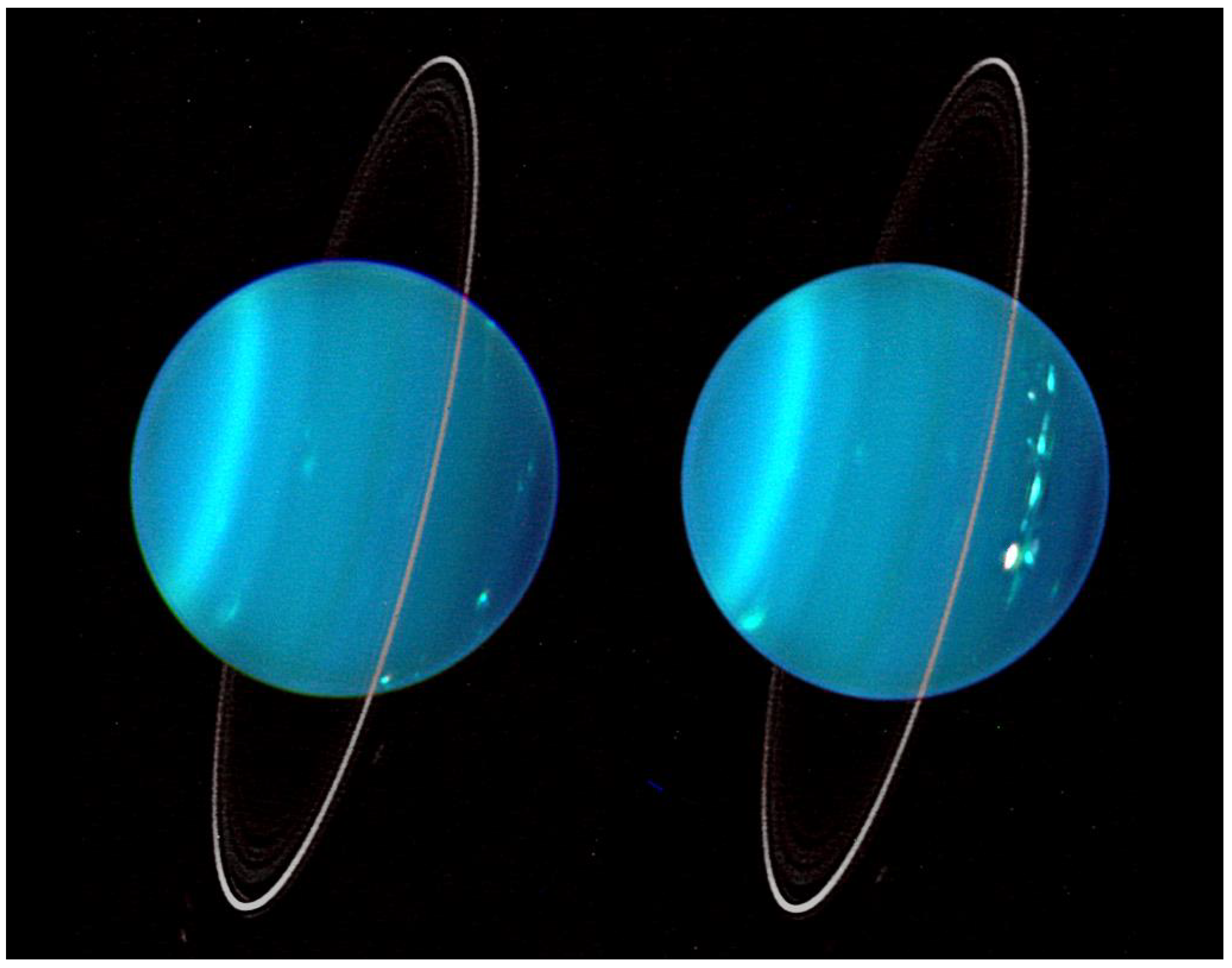
The Berg cloud feature is a distinctive collection of clouds in the southern hemisphere of Uranus that were observed over a 15 year period as described in [1]. While the observations were intermittent and the observed cloud structure somewhat variable, Ref. [1] makes the case for this feature existing continuously over that time period, first as a feature located in the vicinity of −34${}^{\circ }$ (34${}^{\circ }$S) latitude just off the South Polar Collar (SPC) (hence the name “Berg” as if it were an iceberg breaking away from the SPC) (Figure 1), then over the final several years as a feature that drifted from this position towards the equator, with a possible final observation in 2009 at a latitude of −8${}^{\circ }$.

One possible explanation for this feature’s long-lasting coherency and eventual drift is that the Berg is a vortex-cloud system where the clouds are generated by the vortex due to internal circulation, orographic uplift, or other means. The most prominent example of such a system was the 1989 Great Dark Spot observed by Voyager II on Neptune [2]. GDS-89 had a persistent methane cloud companion that existed over an eight-month period of observation as described in [3]. Notably over these eight months, the GDS-89 system appeared to have drifted in latitude from −27${}^{\circ }$ to −17${}^{\circ }$ based first on bright companion cloud and then later on direct vortex observations. More recently a second dark spot on Neptune, SDS-2015, appeared to have drifted a few degrees poleward over two years [4]. While the Berg feature shared the drifting tendencies of these two spots, it did not share an observed dark spot with the clouds. The presumption is that in the case of the Berg clouds and atmosphere above the spot obscured observations of the vortex, or the vortex failed to generate sufficient contrast with the surrounding atmosphere to be detected.

2. Materials and Methods

Numerical simulations of the atmospheric dynamics were conducted using the Explicit Planetary Isentropic Coordinate General Circulation Model (EPIC GCM) [5,6]. The EPIC GCM has been used previously to investigate the morphology and drift of Ice Giant Dark Spots, notably the GDS-89 [7] and the Uranian Dark Spot (UDS) [8]. The governing equations solved by EPIC are a form of the Navier-Stokes equations for oblate spheroids applied to atmospheric layers in the upper troposphere and lower stratosphere of the atmosphere. The layers are defined by a hybrid vertical coordinate that blends a potential temperature coordinate in the upper atmosphere with a pressure-based coordinate in the deeper atmosphere. Based on this previous work, this study simulated the full globe with a grid of 512 × 1024 points (equivalent to a spacing of 0.35${}^{\circ }$ at the equator) along with a 20 layer profile covering depths of a few millibar to approximately 7 bars, extending below the main methane cloud deck at 2–3 bars. The vertical domain and number of layers were defined based on prior Ice Giant vortex simulations, although the number of layers was increased compared to prior UDS simulations [8]. This increase was to provide a sufficient number of layers for reasonable microphysics and separation between the vortex and the top and bottom boundaries. Both the top and bottom layer interface were treated as impermeable. The total grid contained about 10.5 million points.

The initialization of the model required an assumed zonal wind and temperature-pressure profile, both of which are constructed based on observational data. The vertical temperature-pressure profile was initially assumed to be constant across the entire globe. In this case, the profile was the same as that used in the previous UDS simulations [8] based on Voyager 2 occultation data [9] that was extended below pressures of 2 bar by a near-adiabat with a target buoyancy frequency of $N=0.003$ s${}^{-1}$. The zonal wind is assumed uniform with depth. The resulting initial vertical profile is provided in

Table 1. Initial vertical layer structure.

Layer	Hybrid	Pressure	Temperature	Pot. Temp.	N2
1	660.0 K	3.47 mbar	68.4 K	660.0 K	0.000108 s${}^{-2}$
2	477.7 K	7.32 mbar	66.7 K	477.7 K	0.000133 s${}^{-2}$
3	336.7 K	14.4 mbar	61.7 K	336.7 K	0.000165 s${}^{-2}$
4	242.9 K	26.5 mbar	56.8 K	242.9 K	0.000160 s${}^{-2}$
5	185.2 K	46.0 mbar	54.3 K	186.1 K	0.000148 s${}^{-2}$
6	136.8 K	76.6 mbar	53.1 K	148.3 K	0.000146 s${}^{-2}$
7	97.2 K	120.6 mbar	52.9 K	123.4 K	0.000118 s${}^{-2}$
8	92.5 K	180.3 mbar	54.0 K	107.1 K	0.000112 s${}^{-2}$
9	88.3 K	259.1 mbar	55.3 K	94.9 K	0.000099 s${}^{-2}$
10	84.5 K	359.0 mbar	57.5 K	86.6 K	0.000072 s${}^{-2}$
11	81.1 K	481.8 mbar	60.9 K	81.6 K	0.000045 s${}^{-2}$
12	78.1 K	627.8 mbar	65.4 K	78.9 K	0.000024 s${}^{-2}$
13	75.3 K	796.9 mbar	70.6 K	77.5 K	0.000015 s${}^{-2}$
14	72.8 K	987.8 mbar	75.9 K	76.5 K	0.000013 s${}^{-2}$
15	70.3 K	1225 mbar	81.6 K	75.6 K	0.000012 s${}^{-2}$
16	67.6 K	1553 mbar	88.2 K	74.6 K	0.000011 s${}^{-2}$
17	64.4 K	2043 mbar	96.6 K	73.5 K	0.000010 s${}^{-2}$
18	60.6 K	2844 mbar	107.4 K	72.2 K	0.000008 s${}^{-2}$
19	56.0 K	4230 mbar	121.8 K	70.7 K	0.000007 s${}^{-2}$
20	50.4 K	6822 mbar	141.1 K	69.0 K	0.000005 s${}^{-2}$

.

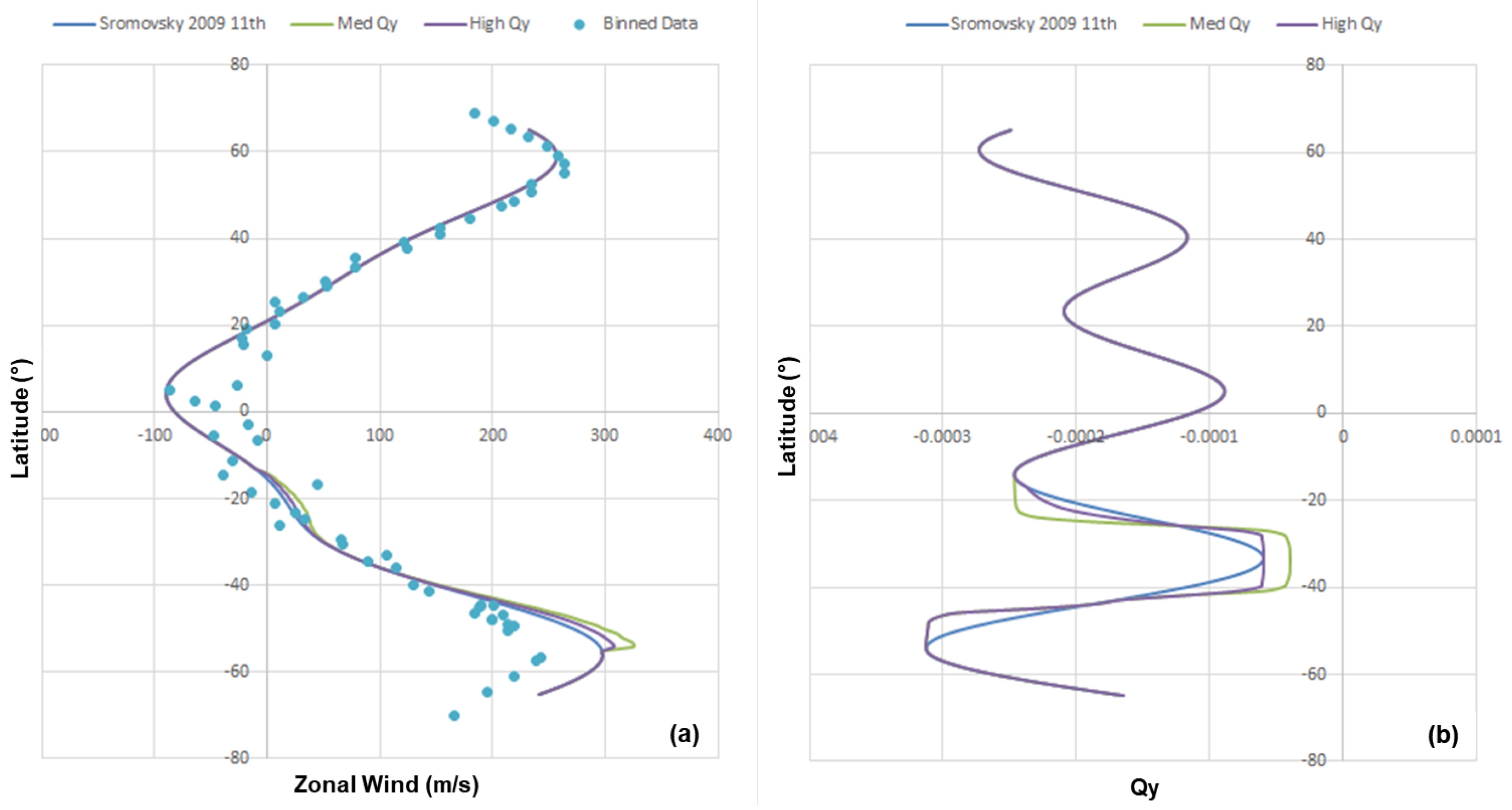
Three zonal wind profiles have been selected for this work, starting with the 11th order Legendre polynomial profile from [10]. The selection of this profile was based on its gradient of absolute vorticity with latitude ($Q_y$) in the vicinity of −34${}^{\circ }$ (Figure 2). Prior work simulating GDS-89 [7] indicated that the drift rate of a dark spot vortex is connected to the value of $Q_y$ in the background atmosphere. Zero gradient was associated with near-zero drift, while larger gradients yielded faster drift rates. This trend is consistent with the beta-gyre theory [11] developed for tropical cyclones, where drift rate is driven by the vortex twisting the surrounding background absolute vorticity gradient into an effective vortex dipole which generates latitudinal motion. Following the approach used in [7,8], the 11th order zonal wind fit was further altered to create a profile with a region of constant $Q_y$ about −34${}^{\circ }$ (High Qy) and a version with a value of $Q_y$ that was even closer to zero (Med Qy). These three profiles were used in this investigation.

Currently, the physical origin of the vortices on the ice giants is not known. Therefore, for these studies, they were induced in the model by introducing vortex-like winds on top of the zonal wind background along with altering the background Montgomery potential in a consistent fashion for an ellipsoidal vortex. However, the quasi-geostrophic balance assumed to generate these vortices is approximate, so the resulting features generally undergo a several simulated day period of adjustment before achieving a more stable state. For this study, a gaussian ellipsoid like that used in [8] for the UDS was employed. In this case, the ellipsoid was defined by an estimated strength of the maximum winds and the major and minor axes of the vortex. This study assumed two spot sizes, 8${}^{\circ }$ × 4${}^{\circ }$, comparable to that used in the UDS study, and a larger version 16${}^{\circ }$ × 8${}^{\circ }$. The vertical gaussian decay scale is 0.5 bar both upward and downward with a central pressure of 1 bar, resulting in an initial spot extending between layer 12 to layer 16 as can be seen in the distribution of relative longitudinal velocities along the minor axis which decay in magnitude moving away from the central layer 14 (Figure 3). Initially, two velocity strengths of 70 m/s and 110 m/s were used, the values corresponding to roughly the maximum relative velocities in the generated vortices in this central layer. Thus, the initial study consisted of 12 simulations (three zonal wind profiles, two spot sizes, and two strengths) with the initial vortex centered at −34${}^{\circ }$ and 1 bar in pressure. Subsequent simulations were conducted based on these initial results, including simulations at different vortex strengths and initial latitudes.

A select subset of the humidity-free simulations were re-simulated including a methane microphysics model. The microphysics model included three phases of methane (vapor, cloud ice, and snow) along with five phase change mechanisms. The parameterization of these phase change processes is described in [13] as successfully applied to Jupiter. The assumption was that initial methane distribution is at a uniform relative humidity, but this will change as the model evolves. Regions of persistent relative humidity 100% or greater became clouds of methane ice following the microphysics model. In this study, the methane was initialized at 40 times solar and 25% relative humidity based on a deep volume mixing ratio of methane of 2.2% [14].

3. Results

Simulation results consist of the initial 12 dry (no microphysics) simulations, additional dry simulations based on the initial results, and simulations with methane microphysics to test cloud formation.

3.1. Initial Simulations

The initial simulations were set to run for 40 terrestrial days (24 h). The first ten days were allotted for the induced vortex to stabilize. Simulations where a coherent vortex failed to survive to day 10 are considered to have no vortex. Otherwise, data analysis began at day 10 and continued until the vortex is no longer detectable in the potential vorticity field or until the end of the simulation. Simulations where the vortex continued to exist for 30 days were extended an additional 30 days. Given this time scale, neither Rayleigh drag zonal wind forcing nor radiative forcing were needed to maintain background conditions.

The results of this initial set of simulations are shown in

Table 2. Results of initial set of dry simulations.

Simulation	Profile	Latitude	Size	Strength	Lifespan	Drift Rate
1	11th order	−34${}^{\circ }$	7.8${}^{\circ }$ × 3.9${}^{\circ }$	70 m/s	60+ days	0.044${}^{\circ }$/day
2	11th order	−34${}^{\circ }$	16.0${}^{\circ }$ × 8.0${}^{\circ }$	70 m/s	20 days	N/A
3	11th order	−34${}^{\circ }$	7.8${}^{\circ }$ × 3.9${}^{\circ }$	110 m/s	60+ days	0.037${}^{\circ }$/day
4	11th order	−34${}^{\circ }$	16.0${}^{\circ }$ × 8.0${}^{\circ }$	110 m/s	50 days	0.145${}^{\circ }$/day
5	High Qy	−34${}^{\circ }$	7.8${}^{\circ }$ × 3.9${}^{\circ }$	70 m/s	50 days	0.078${}^{\circ }$/day
6	High Qy	−34${}^{\circ }$	16.0${}^{\circ }$ × 8.0${}^{\circ }$	70 m/s	No Vortex	N/A
7	High Qy	−34${}^{\circ }$	7.8${}^{\circ }$ × 3.9${}^{\circ }$	110 m/s	60+ days	0.066${}^{\circ }$/day
8	High Qy	−34${}^{\circ }$	16.0${}^{\circ }$ × 8.0${}^{\circ }$	110 m/s	60+ days	0.105${}^{\circ }$/day
9	Med Qy	−34${}^{\circ }$	7.8${}^{\circ }$ × 3.9${}^{\circ }$	70 m/s	No Vortex	N/A
10	Med Qy	−34${}^{\circ }$	16.0${}^{\circ }$ × 8.0${}^{\circ }$	70 m/s	No Vortex	N/A
11	Med Qy	−34${}^{\circ }$	7.8${}^{\circ }$ × 3.9${}^{\circ }$	110 m/s	No Vortex	N/A
12	Med Qy	−34${}^{\circ }$	16.0${}^{\circ }$ × 8.0${}^{\circ }$	110 m/s	No Vortex	N/A

.

For cases where the vortex survived to 60 simulated days, the drift rate is based on the shift in latitude over 60 days. For vortices that lasted between 30 and 60 days, the drift rate is based only on the first 30 days to avoid complications in identifying the vortex center as it dissipates.

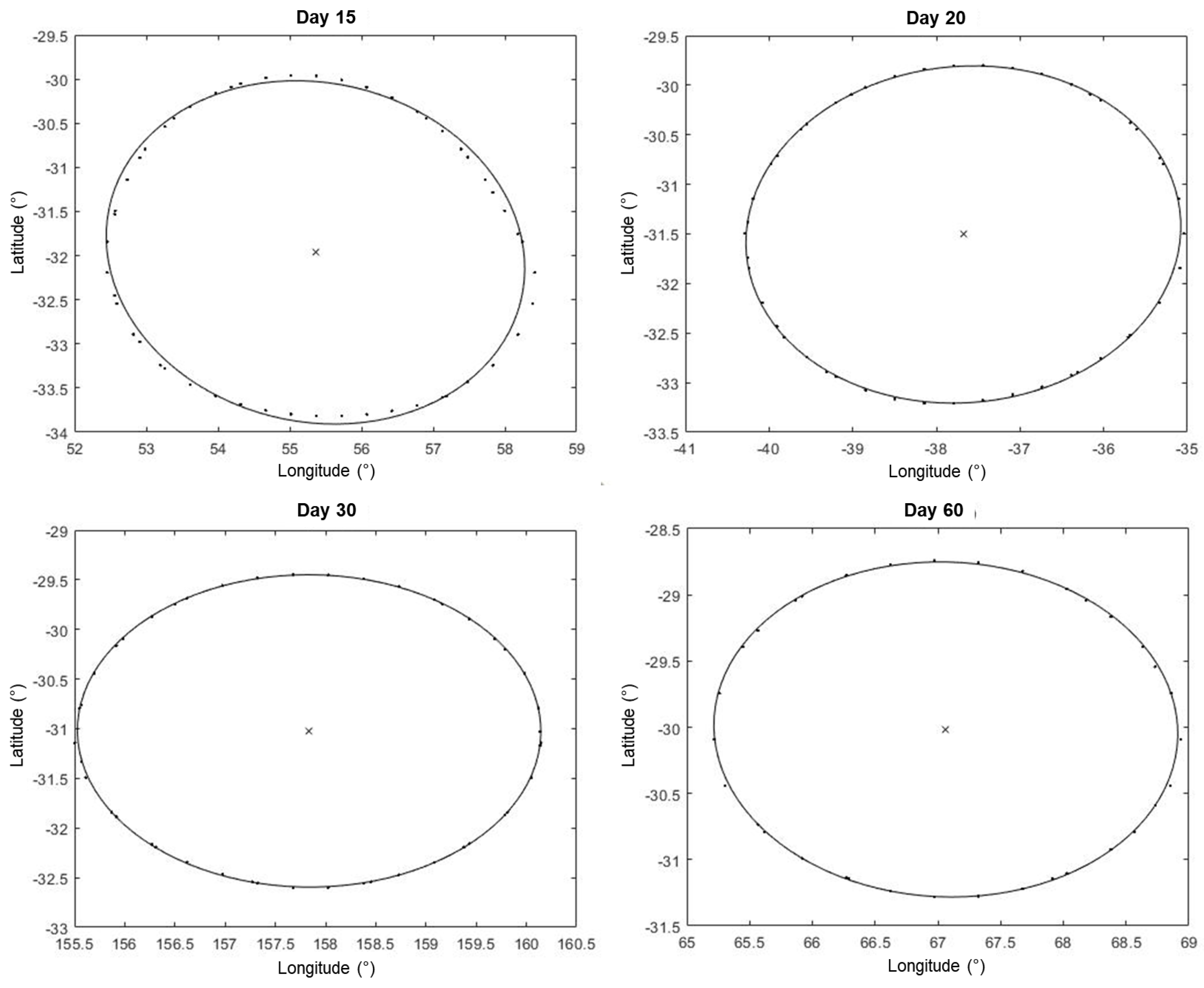
The vortex evolution for Simulations 3 and 7 at a pressure of 700 hPa are provided in Figure 4 and Figure 5. The vortex was defined by an elliptical least-squared fit of points taken from a closed-loop potential vorticity contour. This ellipse was used to define the center of the vortex, in turn defining the latitude of the vortex and thereby the drift rate.

3.2. Additional Dry Simulations

Based on the initial set of simulations, several further simulations were conducted to examine vortex behavior with different strengths and initial latitudes in the Sromovsky 11th order zonal wind profile. These are detailed in

Table 3. Results of additional dry simulations.

Simulation	Profile	Latitude	Size	Strength	Lifespan	Drift Rate
13	11th order	−24${}^{\circ }$	7.8${}^{\circ }$ × 3.9${}^{\circ }$	70 m/s	30+ days	0.22${}^{\circ }$/day
14	11th order	−24${}^{\circ }$	16.0${}^{\circ }$ × 8.0${}^{\circ }$	70 m/s	No Vortex	N/A
15	11th order	−24${}^{\circ }$	7.8${}^{\circ }$ × 3.9${}^{\circ }$	110 m/s	30+ days	0.27${}^{\circ }$/day
16	11th order	−24${}^{\circ }$	16.0${}^{\circ }$ × 8.0${}^{\circ }$	110 m/s	30+ days	0.33${}^{\circ }$/day
17	11th order	−24${}^{\circ }$	7.8${}^{\circ }$ × 3.9${}^{\circ }$	50 m/s	30+ days	0.15${}^{\circ }$/day
18	11th order	−24${}^{\circ }$	7.8${}^{\circ }$ × 3.9${}^{\circ }$	40 m/s	35 days	0.12${}^{\circ }$/day
19	11th order	−24${}^{\circ }$	7.8${}^{\circ }$ × 3.9${}^{\circ }$	30 m/s	No Vortex	N/A
20	11th order	−14${}^{\circ }$	7.8${}^{\circ }$ × 3.9${}^{\circ }$	40 m/s	20 days	0.29${}^{\circ }$/day

.

These simulations investigated vortex behavior at lower vortex strength and at different initial latitudes. The latter allowed for comparisons with the Berg drift at different latitudes, while the former were used to determine the weakest sustainable vortex (about 40 m/s for the cases examined) and to examine if a weaker vortex strength would reduce the drift rate.

3.3. Simulation with Clouds

To test the potential for cloud development, Simulation 7 was redone with the addition of the methane microphysics model. Simulations with methane microphysics are first simulated in two dimensions (latitude and depth) for 200 days to allow the methane distribution to adjust from the uniform initial conditions. This simulation is then extruded to a full globe and then follows the spot-induction procedure of the dry simulations. The overall results of this simulation are given in

Table 4. Results of cloud simulation.

Simulation	Profile	Latitude	Size	Strength	Lifespan	Drift Rate
21	High Qy	−34${}^{\circ }$	7.8${}^{\circ }$ × 3.9${}^{\circ }$	110 m/s	100+ days	0.053${}^{\circ }$/day

, with drift rate based on the first 60 days of the vortex to be consistent with previous calculations.

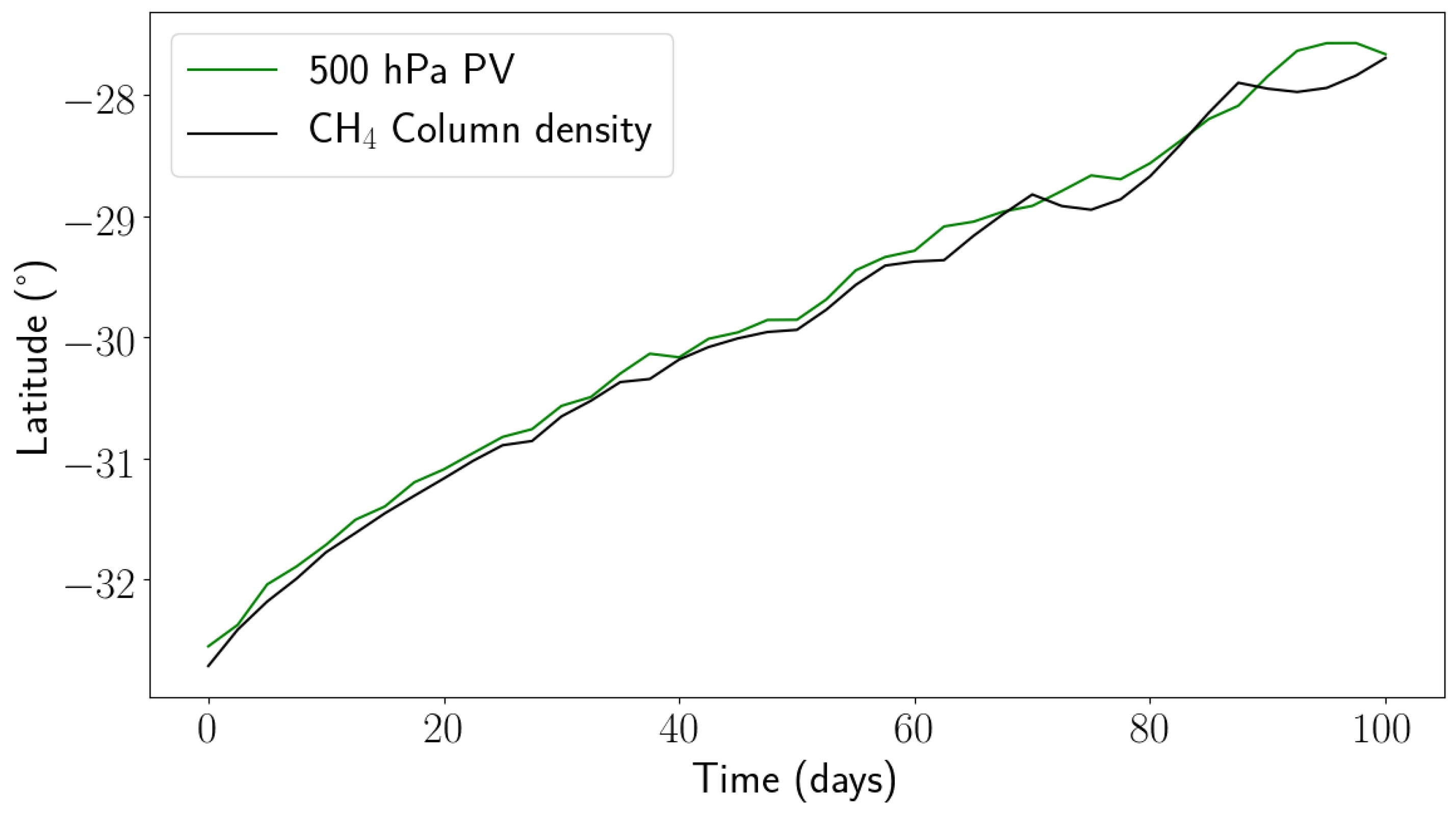
The inclusion of the methane microphysics allows for a deeper investigation of the vortex properties. Figure 6 shows the same four days as Figure 4 and Figure 5, but now the visible spot is defined by methane gas optical depth. The white dashed contour lines define the cloud based on methane ice column density. The green elliptical fit is the potential vorticity definition of the vortex, while the black elliptical fit is based on the methane optical depth. These two definitions yield differences in the drift pattern, but with similar trends (Figure 7).

Figure 8 shows sample vertical-longitudinal velocity fields cut along the central latitude of the vortex and the vertical cloud extent in this plane in conjunction with a latitude-longitude view of the vortex and cloud feature. The cloud is located between the regions of upwelling and downwelling and above the main vortex centered at 1 bar. Figure 9 shows the horizontal velocity field (arrows) and vertical velocity field (colored contours) at 0.5 and 1 bar at day 30. The upwelling and downwelling regions predominantly have a simple east-west dipole pattern, although the exact location shifts with altitude.

4. Discussion

Stable vortices were induced for both the 11th-order and High Qy profiles The initial dry runs suggest that the existence of a region of uniform, lower magnitude $Q_y$ did not enhance the survivability nor increase the likelihood of a vortex in contrast to previous simulations [7,8].

To compare with observations, the Berg was observed at a latitude of −34.4${}^{\circ }$ on 12 August 2004 and then at a latitude of −33.5${}^{\circ }$ on 15 August 2005 [1], corresponding to a drift rate of 0.003${}^{\circ }$/day. This early drift rate is an order of magnitude less than the slowest rates achieved in the simulations. To make a similar comparison at the higher latitudes, using the approximate smooth fit of observed Berg latitudes between 2004 and 2009 in [1] yields a drift rate of 0.02${}^{\circ }$/day at −24${}^{\circ }$ and 0.03${}^{\circ }$/day at −14${}^{\circ }$. Again, the simulated drift rates are roughly an order of magnitude higher at these latitudes. While clearly the current set of simulations does not capture the observed drift rate magnitude, the existing vortices exhibit equatorward drift whose rates tend to accelerate as the equator is approached, consistent with the Berg observations. The general drift pattern is consistent with beta-gyre theory in terms of the equatorward direction and the reduced drift rate with lower vortex strength for the −24${}^{\circ }$ simulations. The only vortex to approach the equator, Simulation 20, did dissipate at about −8${}^{\circ }$, comparable to the possible final Berg observation.

The addition of methane to the simulation did not, in the case tested here, reduce the drift rate to levels comparable to observations, yielding a 0.053${}^{\circ }$/day drift compared to the 0.066${}^{\circ }$/day drift for the corresponding dry case (Simulation 7). The velocity fields for Simulation 21 reveal a persistent circulation pattern with upwelling on the western half of the vortex and downwelling on the eastern. However, the driving mechanism of the circulation and its relationship to companion cloud formation require further investigation. This dark spot does not generate the quadrupole pattern in the vertical wind structure seen in comparable simulations of the Great Red Spot of Jupiter due to that vortex residing in a pair of opposing background jets [15]. In many cases, the ice cloud did cover a substantial portion of the vortex, although the degree of that coverage was variable over time. Berg observations prior to 2005 were characterized by [10] as having clouds covering 10 to 20 degrees in latitude, while the simulated cloud reached about six degrees in extent.

Further refinement of the parameter space may provide more precise matches to the Berg observations. Several parameters such as the temperature-pressure profile, the vertical wind shear, and the initial methane humidity were not varied in the current study, which focused on the effects of zonal wind shear and vortex conditions. In addition, these initial simulations were conducted using a methane microphysics model and a dark spot in the vicinity of 1 bar, comparable to previous dark spot studies, but Ref. [1] noted the likelihood that a non-methane trace gas forms many of the Berg clouds, with one suggestion being hydrogen sulfide. This in turn suggests that the driving vortex may be deeper (2–3 bars). If the zonal winds weaken with depth, a deeper vortex may exhibit lower drift rates. Investigating this possibility along with the effects of other key parameters will be the subject of future work.