An Integrated Wind Risk Warning Model for Urban Rail Transport in Shanghai, China

 ,
,
Abstract
1. Introduction
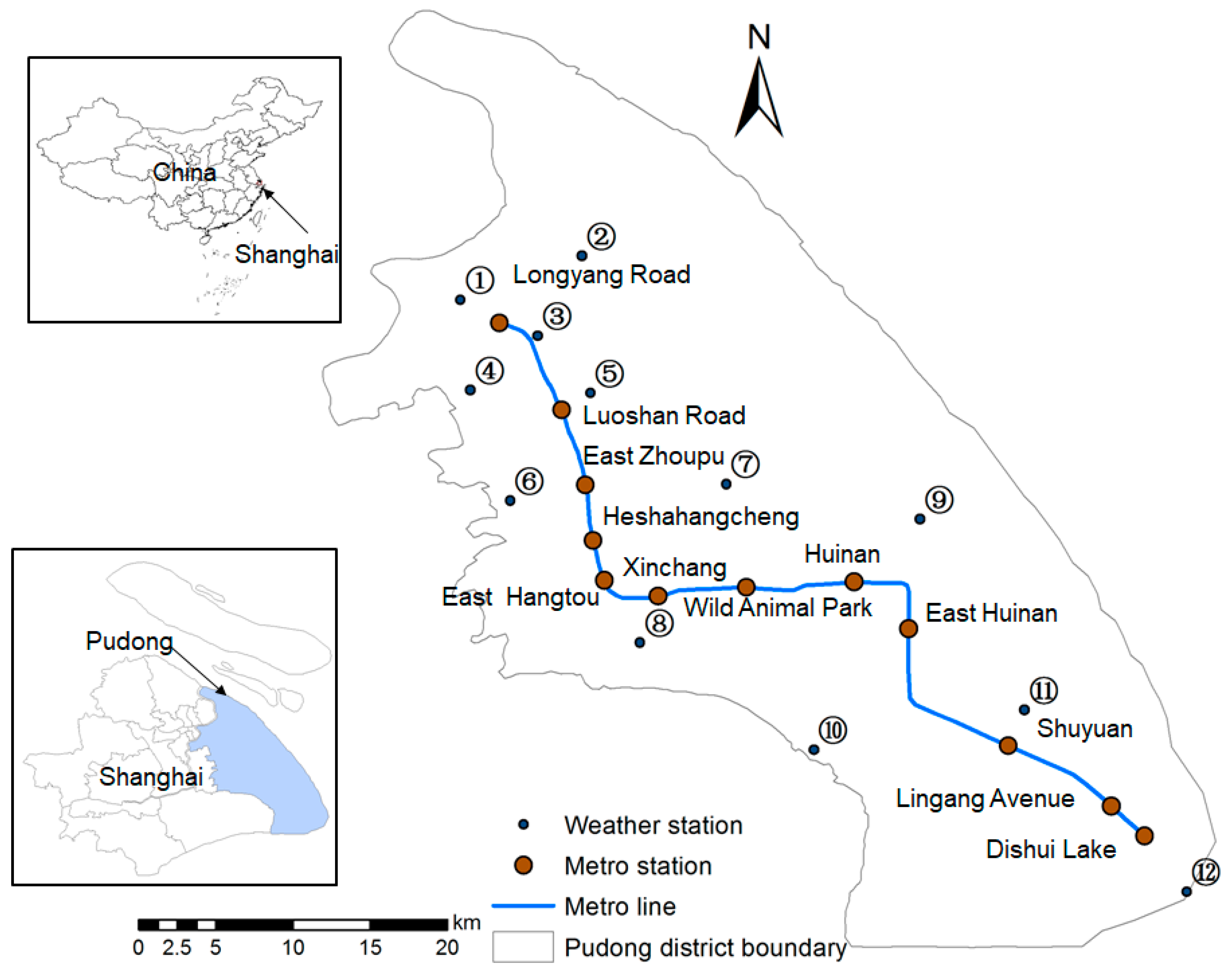
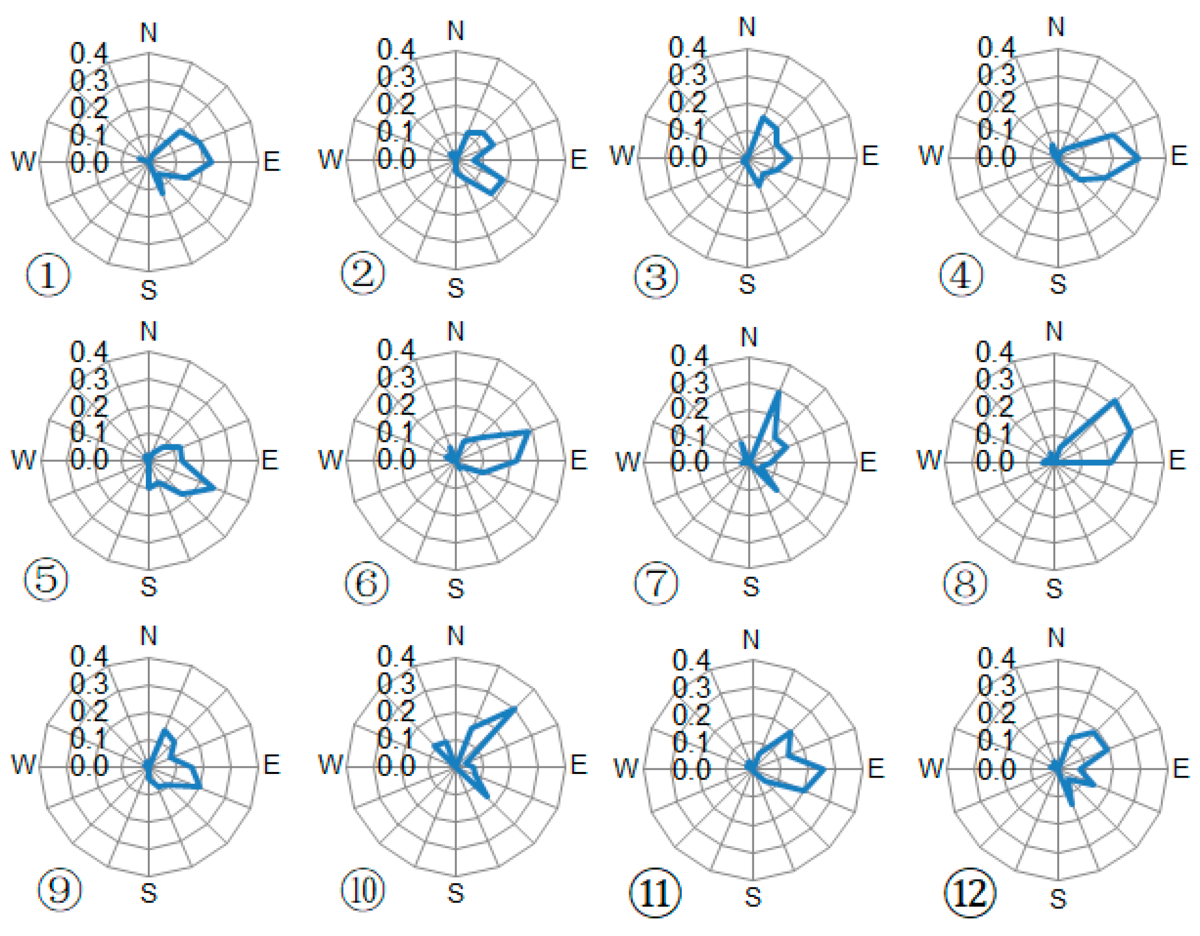
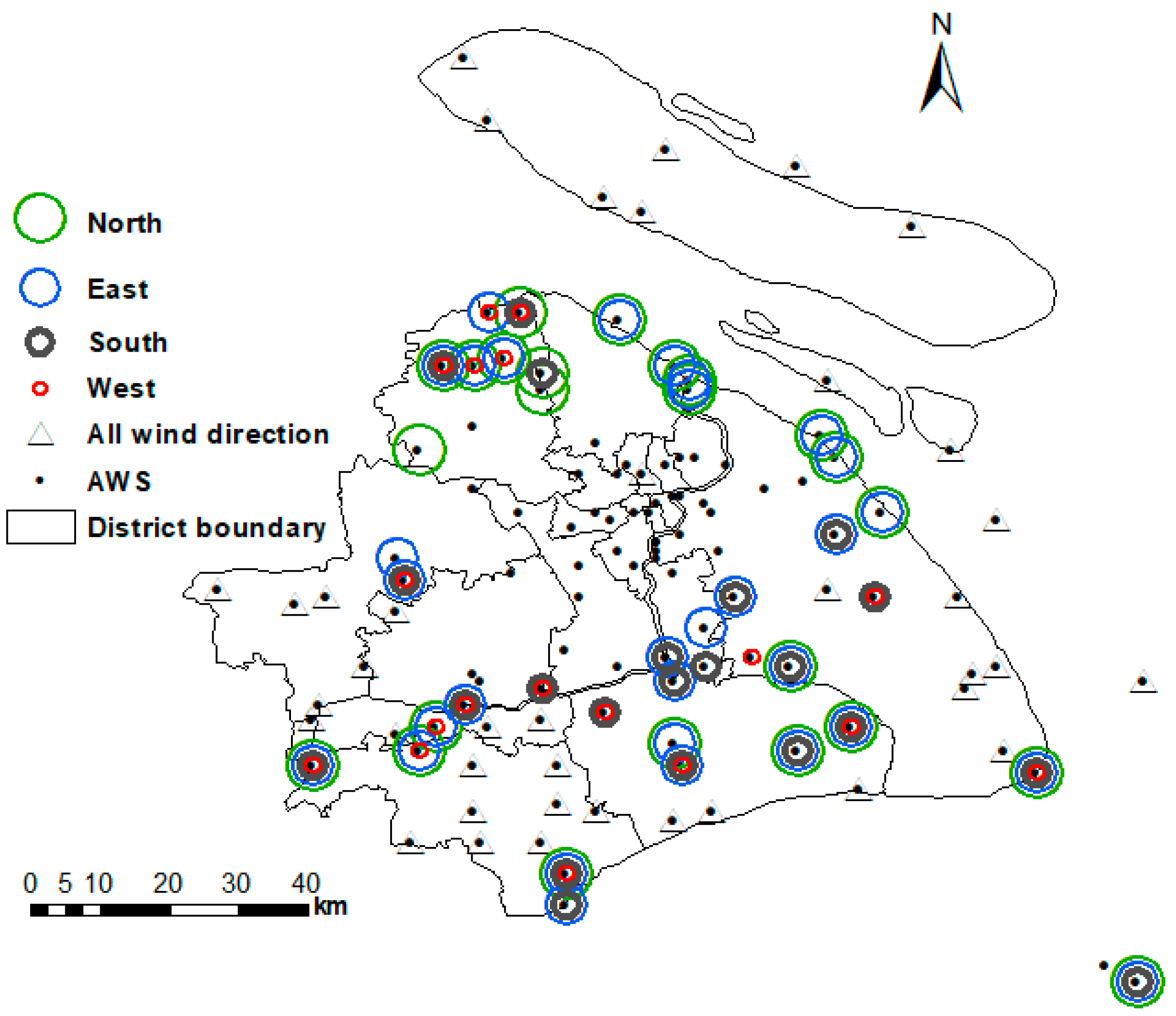
2. Meteorological Background
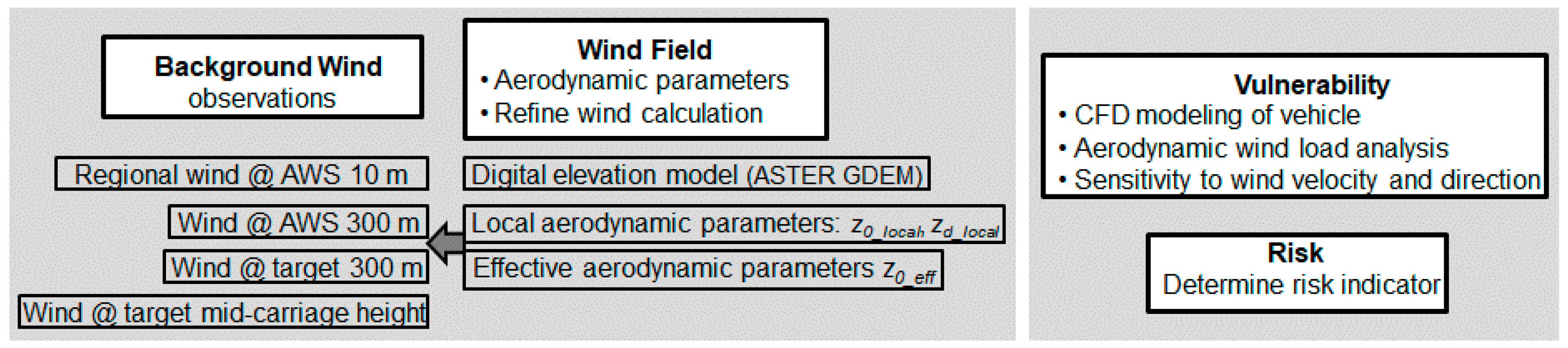
3. Methodology
- Background wind determined from numerical weather prediction (NWP) or observations (used here) to create a high-resolution wind field.
- Vulnerability model to calculate the influence of the wind load on rail carriages.
- Risk model to develop a warning.
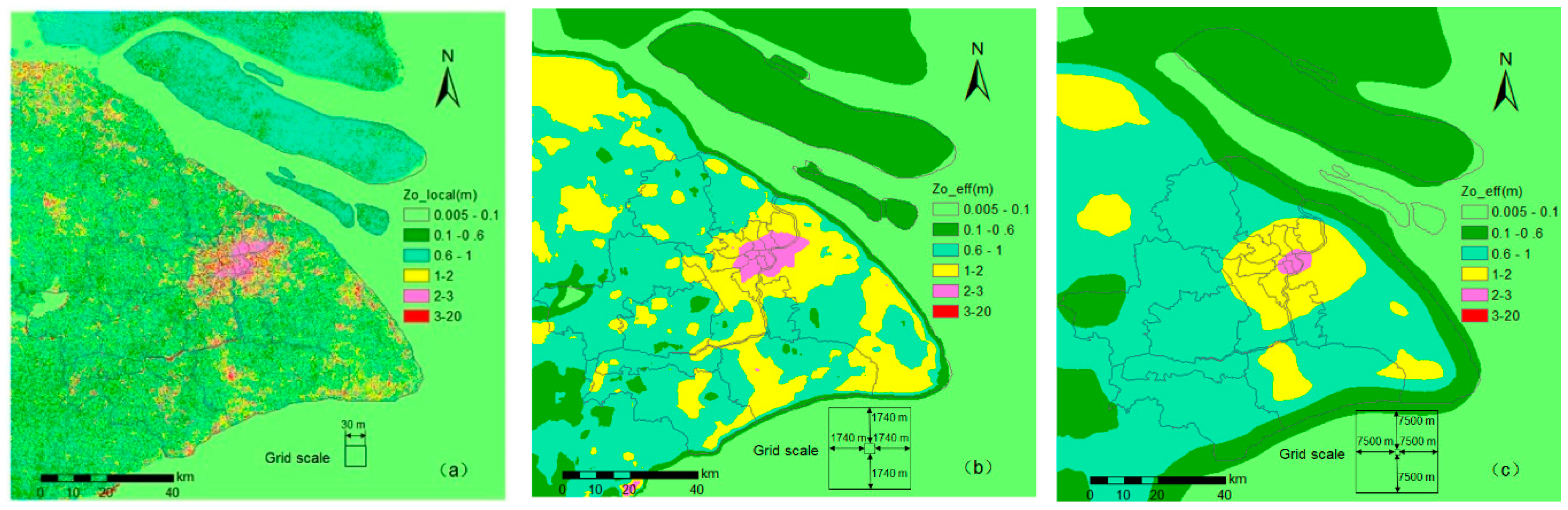
3.1. Wind Field
3.2. Vulnerability Model
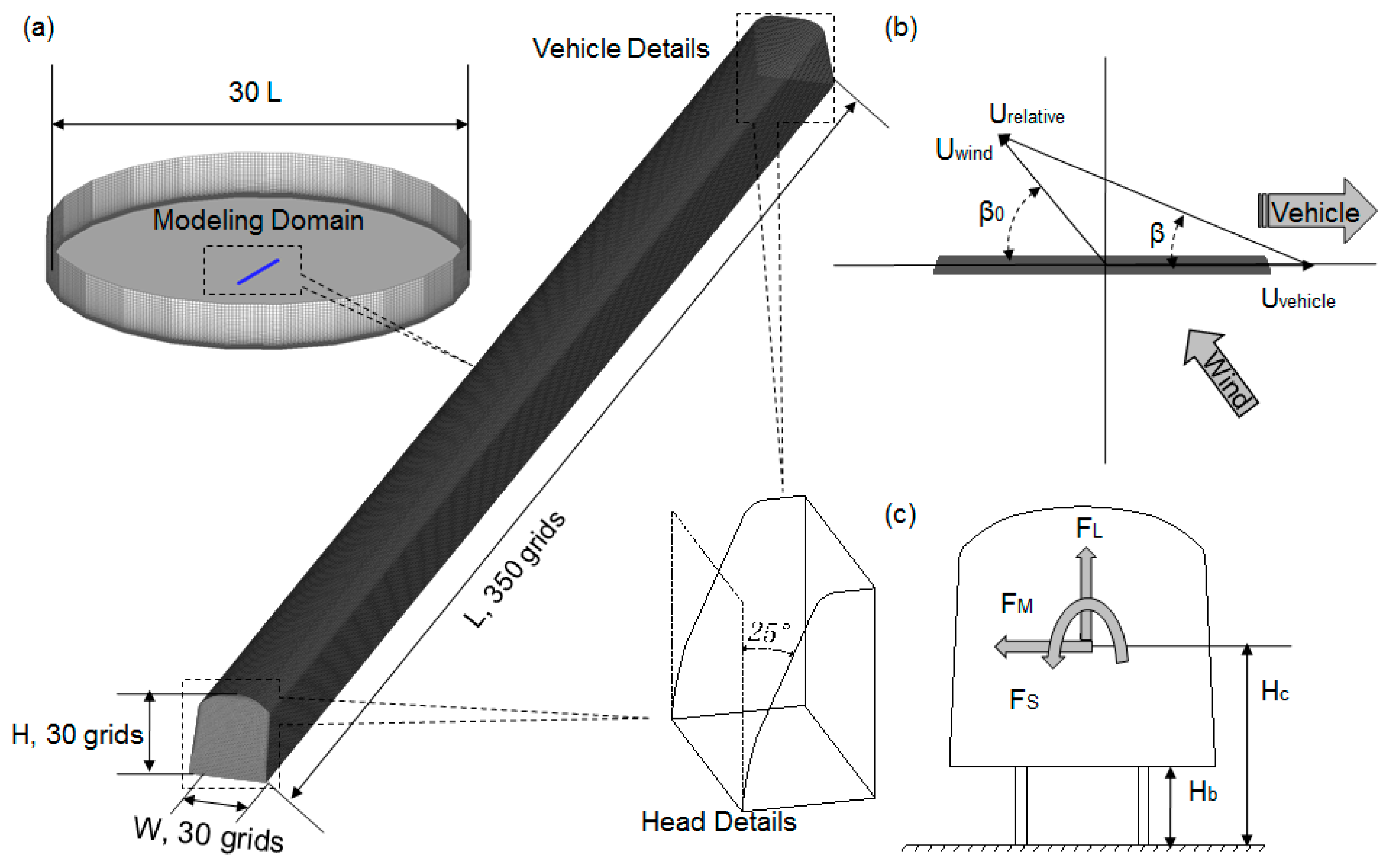
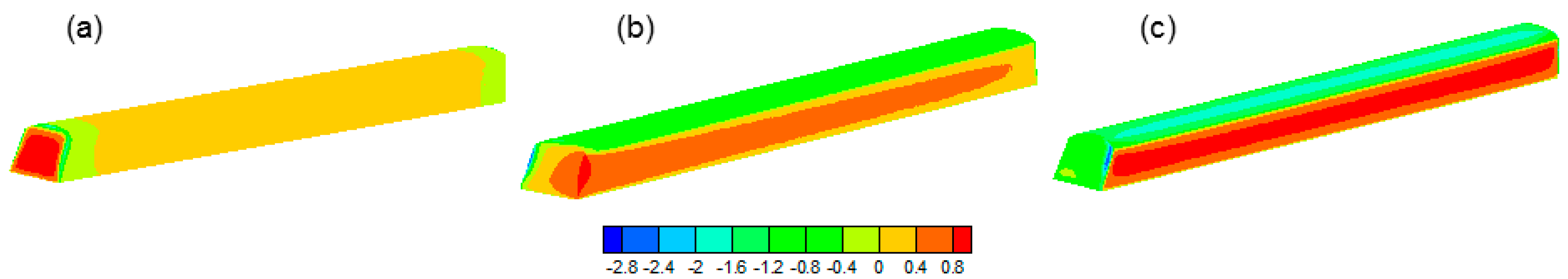
3.2.1. Wind load Modeling
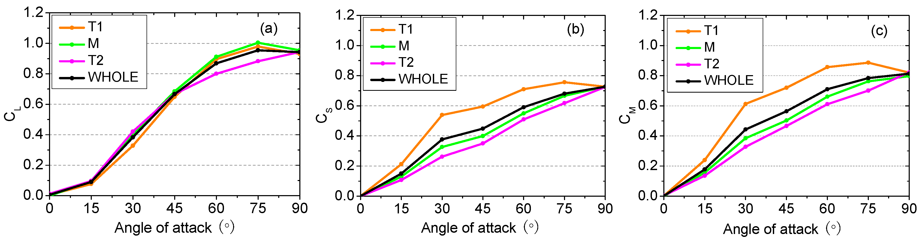
3.2.2. Effect of Angle of Attack
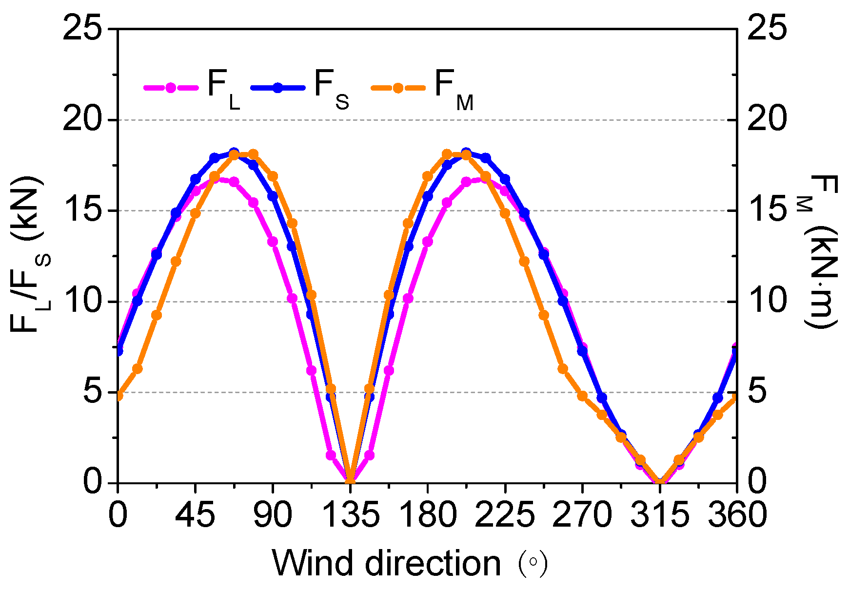
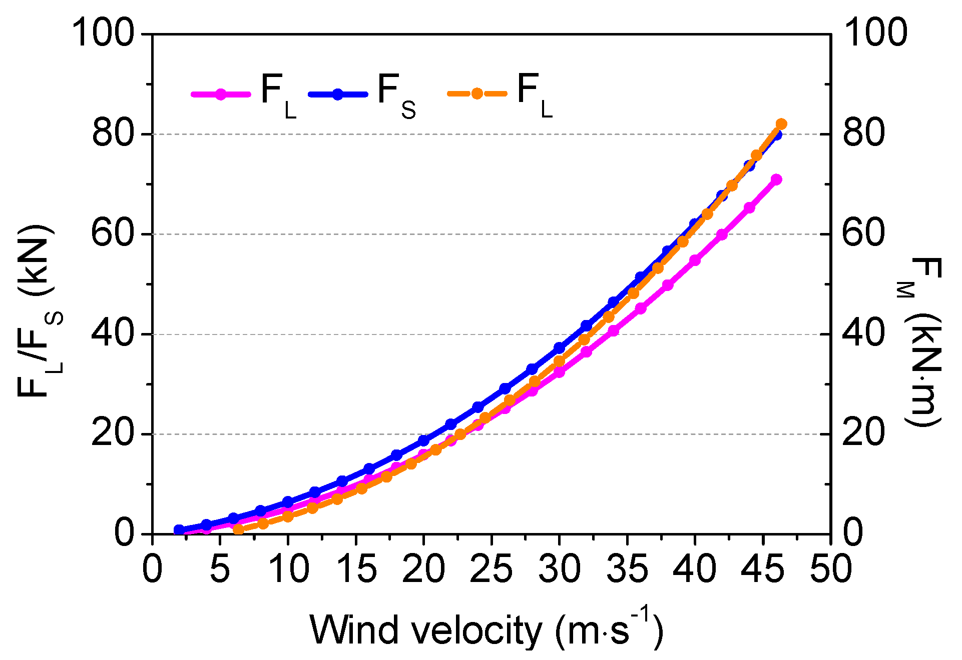
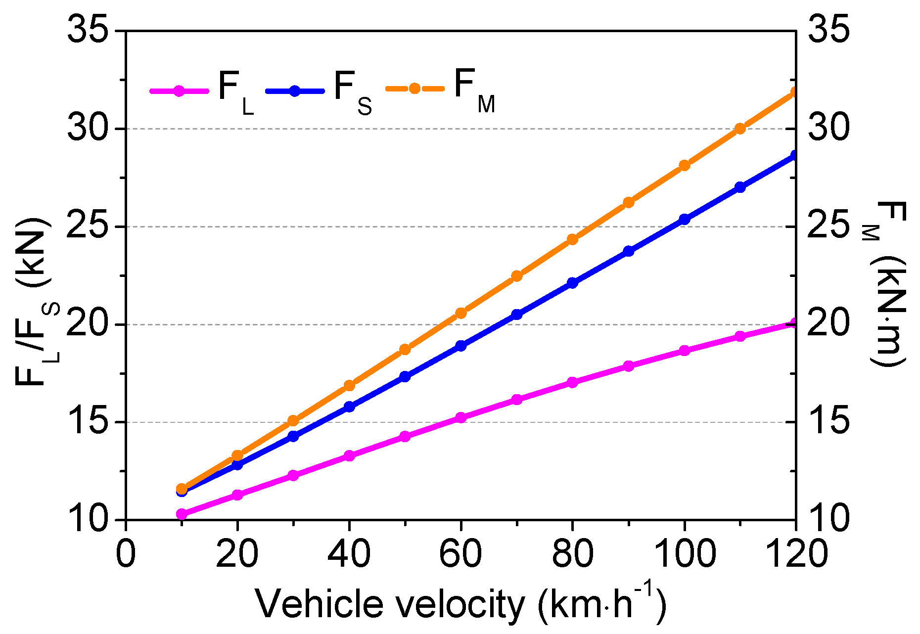
3.2.3. Effect of Wind Direction, Wind Velocity, and Vehicle Velocity
3.3. Risk Model
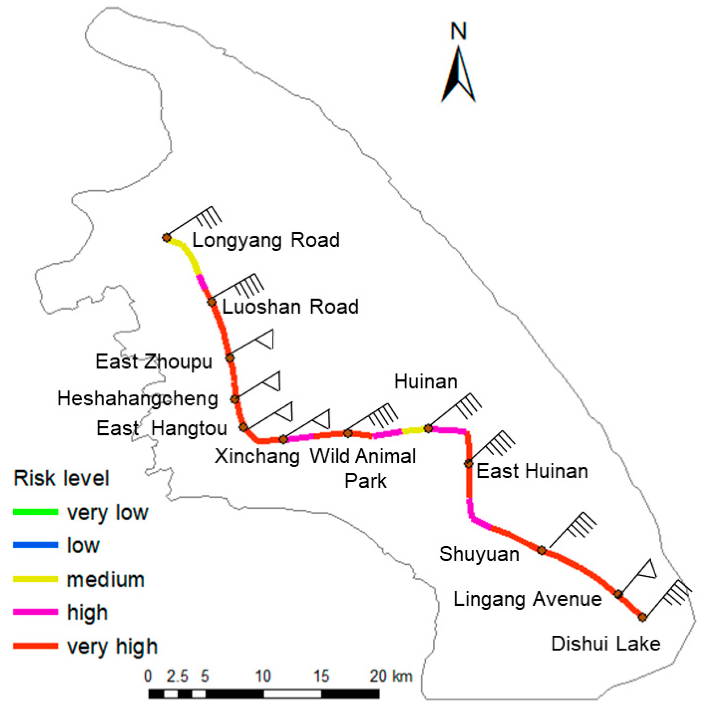
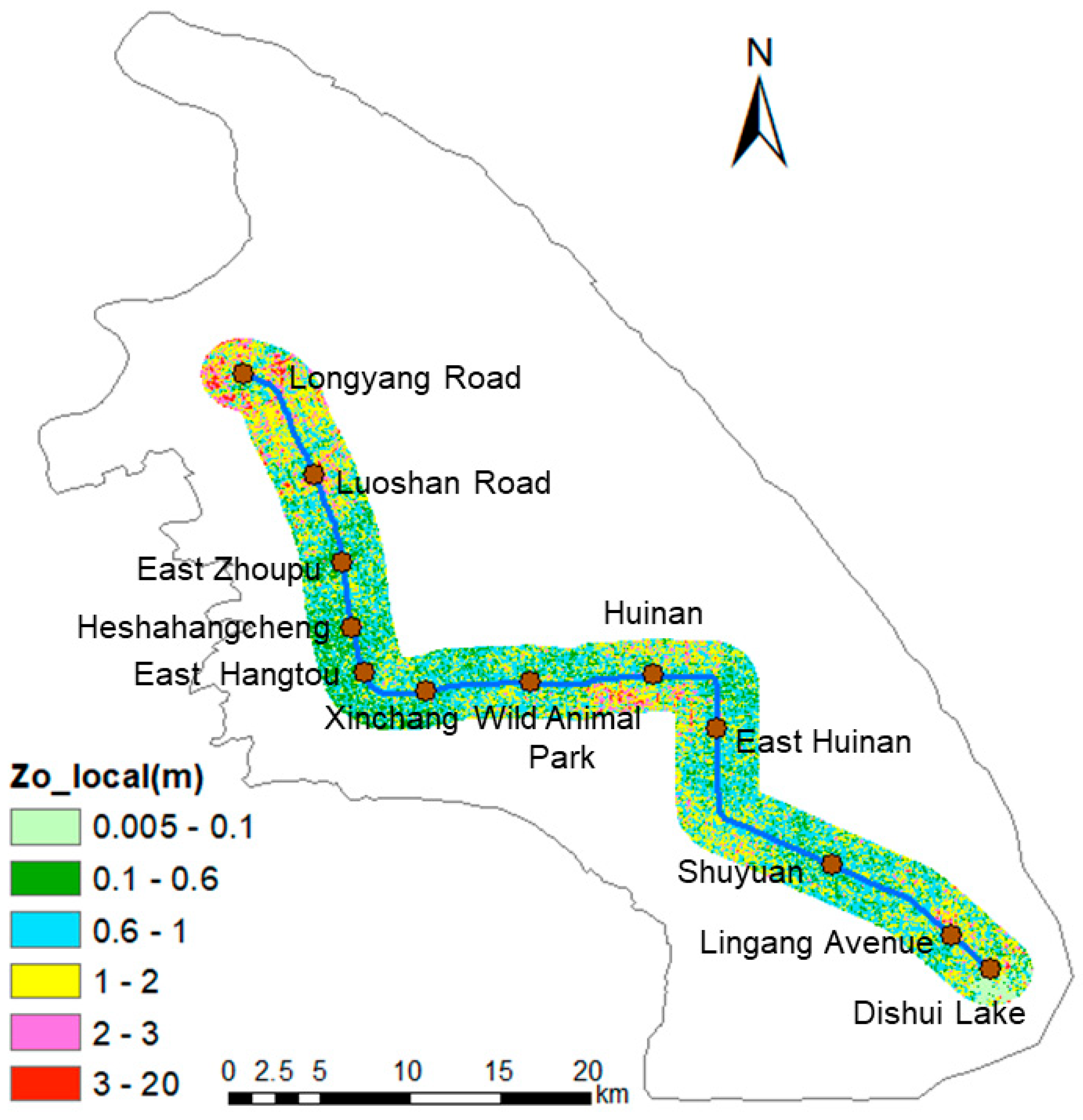
4. Application
5. Conclusions
Author Contributions
Funding
Acknowledgments
Conflicts of Interest
References
- Ludvigsen, J.; Klæboe, R. Extreme weather impacts on freight railways in Europe. Nat. Hazards 2014, 70, 767–787. [Google Scholar] [CrossRef]
- Vajda, A.; Tuomenvirta, H.; Juga, I.; Nurmi, P.; Jokinen, P.; Rauhala, J. Severe weather affecting European transport systems: The identification, classification and frequencies of events. Nat. Hazards 2014, 72, 169–188. [Google Scholar] [CrossRef]
- Jaroszweski, D.; Hooper, E.; Baker, C.; Chapman, L.; Quinn, A. The impacts of the 28 June 2012 storms on UK road and rail transport. Meteorol. Appl. 2015, 22, 470–476. [Google Scholar] [CrossRef]
- The Pujiang Line Began to Operate on 31 March. Available online: http://www.shmetro.com/node49/201803/con115042.htm (accessed on 20 June 2018). (In Chinese).
- Weng, C. Application of strong wind forecast on Shanghai rail transit elevated and ground metro lines. Urban Mass Transit. 2016, 19, 138–142. (In Chinese) [Google Scholar]
- Zhang, W. Rethink about work of ‘9.13’ rainstorm and ‘Feite’ typhoon. Urban Roads Bridges Flood Control 2015, 36, 127–129. (In Chinese) [Google Scholar]
- “Haikui” Slams Shanghai Making Suspension of High-Speed Rail and Maglev. Available online: http://bj.bendibao.com/news/201289/82662.shtm (accessed on 30 December 2019). (In Chinese).
- Suarez, P.; Anderson, W.; Mahal, V.; Lakshmanan, T.R. Impacts of flooding and climate change on urban transportation: A systemwide performance assessment of the Boston Metro Area. Transp. Res. Part D 2005, 10, 231–244. [Google Scholar] [CrossRef]
- Koetse, M.J.; Rietveld, P. The impact of climate change and weather on transport: An overview of empirical findings. Transp. Res. Part D 2009, 14, 205–221. [Google Scholar] [CrossRef]
- Jaroszweski, D.; Chapman, L.; Petts, J. Assessing the potential impact of climate change on transportation: The need for an interdisciplinary approach. J. Transp. Geogr. 2010, 18, 331–335. [Google Scholar] [CrossRef]
- Ferranti, E.; Chapman, L.; Lowe, C.; Mcculloch, S.; Jaroszweski, D.; Quinn, A. Heat-related failures on southeast England’s railway network: Insights and implications for heat risk management. Weather Clim. Soc. 2016, 8, 177–191. [Google Scholar] [CrossRef]
- Tsubaki, R.; Kawahara, Y.; Ueda, Y. Railway embankment failure due to ballast layer breach caused by inundation flows. Nat. Hazards 2017, 87, 717–738. [Google Scholar] [CrossRef]
- A Train in Xinjiang is Struck by a Thirteen-Grade Gale, Causing Carriages Rollover and Three People Deaths. Available online: http://news.sina.com.cn/c/2007-02-28/083812389192.shtml (accessed on 5 June 2013). (In Chinese).
- Brockie, N.J.W.; Baker, C.J. The Aerodynamic Drag of High Speed Trains. J. Wind Eng. Ind. Aerodyn. 1990, 34, 273–290. [Google Scholar] [CrossRef]
- Tian, H.; Gao, G. The analysis and evaluation on the aerodynamic behavior of 270 km/h high-speed train. China Railw. Sci. 2003, 24, 14–18. (In Chinese) [Google Scholar]
- Bocciolone, M.; Cheli, F.; Corradi, R.; Muggiasca, S.; Tomasini, G. Crosswind action on rail vehicles: Wind tunnel experimental analyses. J. Wind Eng. Ind. Aerodyn. 2008, 96, 584–610. [Google Scholar] [CrossRef]
- Carrarini, A. Reliability based analysis of the crosswind stability of railway vehicles. J. Wind Eng. Ind. Aerodyn. 2006, 95, 493–509. [Google Scholar] [CrossRef]
- Xi, Y. Research on Aerodynamic Characteristics and Operation Safety of High-Speed Trains under Cross Winds. Ph.D. Thesis, Beijing Jiaotong University, Beijing, China, 2012. [Google Scholar]
- Huang, S.K.; Lindell, M.K.; Prater, C.S.; Wu, H.; Siebeneck, L.K. Household evacuation decision making in response to Hurricane Ike. Nat. Hazards Rev. 2012, 13, 283–296. [Google Scholar] [CrossRef]
- Meyer, R.; Broad, K.; Orlove, B.; Petrovic, N. Dynamic simulation as an approach to understanding hurricane risk response: Insights from the Storm view lab. Risk Anal. 2013, 33, 1532–1552. [Google Scholar] [CrossRef]
- Bostrom, A.; Morss, R.E.; Lazo, J.K.; Demuth, J.L.; Lazrus, H.; Hudson, R. A mental models study of hurricane forecast and warning production, communication, and decision-making. Weather Clim. Soc. 2016, 8, 111–129. [Google Scholar] [CrossRef]
- Baker, C.J.; Jones, J.; Lopez-Calleja, F.; Munday, J. Measurements of the cross-wind forces on trains. J. Wind Eng. Ind. Aerodyn. 2004, 92, 547–563. [Google Scholar] [CrossRef]
- Shanghai Statistics Bureau. 2016 Shanghai Statistical Yearbook (in Chinese); China Statistics Press: Beijing, China, 2016.
- Shi, J.; Xu, J.; Tan, J.; Liu, J. Estimation of wind speeds for different recurrence intervals in Shanghai. Sci. Geogr. Sin. 2015, 35, 1191–1197. (In Chinese) [Google Scholar]
- WMO Typhoon Committee. Typhoon Committee Operational Manual Meteorological Component, 2012 ed.; World Meteorological Organization, Tropical Cyclone Programme Report No. TCP-23, WMO/TD-No. 196; World Meteorological Organization: Geneva, Switzerland, 2012. [Google Scholar]
- NASA/METI. Advanced Spaceborne Thermal Emission and Reflection Radiometer Global Digital Elevation Model: ASTER DEM V1. GDC Computer Network Information Center, Chinese Academy of Sciences. Available online: http://www.nasa.com (accessed on 15 October 2016).
- Garratt, J.R. The Atmospheric Boundary Layer; Cambridge University Press: Cambridge, UK, 1992. [Google Scholar]
- Raupach, M.R. Drag and drag partition on rough surfaces. Boundary-Layer Meteorol. 1992, 60, 375–395. [Google Scholar] [CrossRef]
- Hanna, S.R.; Chang, J.C. Boundary layer parameterization for applied dispersion modeling over urban areas. Boundary-Layer Meteorol. 1992, 58, 229–259. [Google Scholar] [CrossRef]
- Grimmond, C.S.B.; Oke, T.R. Aerodynamic properties of urban areas derived from analysis of surface form. J. Appl. Meteorol. 1999, 38, 1262–1292. [Google Scholar] [CrossRef]
- Kent, C.W.; Grimmond, S.; Barlow, L.; Gatey, D.; Kotthaus, S.; Lindberg, F.; Halios, C.H. Evaluation of urban local-scale aerodynamic parameters: Implications for the vertical profile of wind speed and for source areas. Boundary-Layer Meteorol. 2017, 164, 183–213. [Google Scholar] [CrossRef]
- Tennekes, H. The logarithmic wind profile. J. Atmos. Sci. 1973, 30, 234–238. [Google Scholar] [CrossRef]
- USGS. Shuttle Radar Topography Mission Documentation: SRTM3. GDC Computer Network Information Center, Chinese Academy of Sciences. Available online: http://www.gscloud.cn (accessed on 30 October 2016).
- WMO. Guide to Meteorological Instruments and Methods of Observation. 2014 ed. World Meteorological Organization. Available online: https://library.wmo.int/opac/doc_num.php?explnum_id=3121 (accessed on 13 October 2016).
- Shepard, D. A two-dimensional interpolation function for irregularly-spaced data. In Proceedings of the 23rd National Conference of the Association for Computing Machinery, Princeton, NJ, USA, 27–29 August 1968; pp. 517–524. [Google Scholar]
- Wieringa, J. Roughness-dependent geographical interpolation of surface wind speed averages. Q. J. R. Meteorol. Soc. 1986, 112, 867–889. [Google Scholar] [CrossRef]
- Macdonald, R.W. Modeling the mean velocity profile in the urban canopy layer. Boundary-Layer Meteorol. 2000, 97, 25–45. [Google Scholar] [CrossRef]
- García, J.; Muñoz-Paniagua, J.; Jiménez, A.; Migoya, E.; Crespo, A. Numerical study of the influence of synthetic turbulent inflow conditions on the aerodynamics of a train. J. Fluids Struct. 2015, 56, 134–151. [Google Scholar] [CrossRef]
- Fang, P.; Gu, M.; Tan, J. Numerical wind fields based on the k-ε turbulent models in computational wind engineering. China J. Hydrodyn. 2010, 25, 475–483. (In Chinese) [Google Scholar]
- Shih, T.; Liou, W.W.; Shabbir, A.; Yang, Z.; Zhu, J. A new k–ε eddy viscosity model for high Reynolds number turbulent flows. Comput. Fluids 1995, 24, 227–238. [Google Scholar] [CrossRef]
- Vandoormaal, J.P.; Raithby, G.D. Enhancements of the SIMPLE Method for Predicting Incompressible Fluid Flows. Numer. Heat Transfer Appl. 1984, 7, 147–163. [Google Scholar]
- Patankar, S.V. Numerical Heat Transfer and Fluid Flow; Taylor & Francis: London, UK, 1980. [Google Scholar]
- Leonard, B.P.; Mokhtari, S. ULTRA-SHARP Non-Oscillatory Convection Schemes for High-Speed Steady Multi-Dimensional Flow; NASA Technical Memorandum 102568 (ICOMP-90-12) 1990; NASA: Washington, DC, USA, 1990.


| Year | TC Code | Name | Time affected Shanghai (LST) | N |
|---|---|---|---|---|
| 2005 | 0509 | Matsa | 5 Aug, 05:00–7 Aug, 23:00 | 67 |
| 2005 | 0515 | Khanun | 9 Sep, 11:00–16:00 | 8 |
| 2006 | 0601 | Chanchu | 18 May, 08:00–17:00 | 10 |
| 2006 | 0604 | Bilis | 14 Jul, 06:00–15 Jul, 16:00 | 35 |
| 2007 | 0713 | Wipha | 19 Sep, 00:00–20:00 | 21 |
| 2007 | 0716 | Krosa | 6 Oct, 12:00–21:00 7 Oct, 20:00–8 Oct, 22:00 | 37 |
| 2011 | 1109 | Muifa | 6 Aug, 10:00–7 Aug, 16:00 | 31 |
| 2012 | 1209 | Saola | 3 Aug, 05:00–12:00 | 8 |
| 2012 | 1211 | Haikui | 6 Aug, 08:00–9 Aug, 05:00 | 70 |
| 2012 | 1215 | Bolaven | 27 Aug, 03:00–28 Aug,02:00 | 24 |
| Range | 0 < R ≤ 0.25 | 0.25 < R ≤ 0.5 | 0.5 < R ≤ 0.75 | 0.75 < R ≤ 1 | R > 1 |
|---|---|---|---|---|---|
| Risk Level | Very low | Low | Medium | High | Very high |
| Minimum Wind Velocity (m·s−1) | - | 7.0 | 11.9 | 15.7 | 18.0 |
© 2020 by the authors. Licensee MDPI, Basel, Switzerland. This article is an open access article distributed under the terms and conditions of the Creative Commons Attribution (CC BY) license (http://creativecommons.org/licenses/by/4.0/).
Share and Cite
Han, Z.; Tan, J.; Grimmond, C.S.B.; Ma, B.; Yang, T.; Weng, C. An Integrated Wind Risk Warning Model for Urban Rail Transport in Shanghai, China. Atmosphere 2020, 11, 53. https://doi.org/10.3390/atmos11010053
Han Z, Tan J, Grimmond CSB, Ma B, Yang T, Weng C. An Integrated Wind Risk Warning Model for Urban Rail Transport in Shanghai, China. Atmosphere. 2020; 11(1):53. https://doi.org/10.3390/atmos11010053
Chicago/Turabian StyleHan, Zhihui, Jianguo Tan, C. S. B. Grimmond, Bingxin Ma, Tongxiao Yang, and Chunhui Weng. 2020. "An Integrated Wind Risk Warning Model for Urban Rail Transport in Shanghai, China" Atmosphere 11, no. 1: 53. https://doi.org/10.3390/atmos11010053
APA StyleHan, Z., Tan, J., Grimmond, C. S. B., Ma, B., Yang, T., & Weng, C. (2020). An Integrated Wind Risk Warning Model for Urban Rail Transport in Shanghai, China. Atmosphere, 11(1), 53. https://doi.org/10.3390/atmos11010053