Article

Inferring Fine-Mode and Coarse-Mode Aerosol Complex Refractive Indices from AERONET Inversion Products over China

1
School of Energy Science and Engineering, Harbin Institute of Technology, 92 West Dazhi Street, Harbin 150001, China
2
Key Laboratory of Aerospace Thermophysics, Ministry of Industry and Information Technology, Harbin Institute of Technology, 92 West Dazhi Street, Harbin 150001, China
*
Author to whom correspondence should be addressed.
Atmosphere 2019, 10(3), 158; https://doi.org/10.3390/atmos10030158
Submission received: 31 January 2019 / Revised: 13 March 2019 / Accepted: 19 March 2019 / Published: 25 March 2019
(This article belongs to the Special Issue Atmospheric Aerosol Regional Monitoring)

Abstract

:
Detailed knowledge of the complex refractive indices (m) of fine- and coarse-mode aerosols is important for enhancing understanding of the effect of atmospheric aerosol on climate. However, studies on obtaining aerosol modal m values are particularly scarce. This study proposes a method for inferring m values of fine- and coarse-mode aerosol using the inversion products from the AERONET ground-based aerosol robotic network. By identifying the aerosol type, modal m values are constrained and then inferred based on a maximum likelihood method. Numerical tests showed that compared with the reference values, our method slightly overestimates the real parts of the refractive indices (n), but underestimates the imaginary parts (k) by 2.11% ± 11.59% and 8.4% ± 26.42% for fine and coarse modes, respectively. We applied this method to 21 AERONET sites around China, which yielded annual mean m values of (1.45 ± 0.04) + (0.0109 ± 0.0046)i and (1.53 ± 0.01) + (0.0039 ± 0.0011)i for fine- and coarse-mode aerosols, respectively. It is observed that the fine mode n decreased from 1.53 to 1.39 with increasing latitude, while fine mode k values were generally larger than 0.008 over most of China. The coarse-mode n and k ranged from 1.52 to 1.56 and from 0.002 to 0.006, respectively.

Graphical Abstract

1. Introduction

Atmospheric aerosol plays an important role in the Earth-Ocean-Atmosphere system because it changes the radiance balance of the system via both direct effects, such as absorption and scattering of shortwave solar radiation and longwave earth radiation, and indirect effects, such as acting as cloud condensation nuclei [1,2]. The complex refractive index is a fundamental parameter in determining the absorption and scattering properties of atmospheric aerosols and is the basis for calculating the earth’s radiative budget and assessing the aerosol climate effect [3,4,5]. The complex refractive index can be mathematically described as m = n + ki, where the real part n represents the light scattering capacity of aerosol particles, while the imaginary part k is related to the light absorption capacity [6,7,8,9]. The overall m value depends on the chemical composition, it is directly related to the emission source, and can be characterized by the typical particle modes, i.e., fine and coarse modes [8,10,11,12]. For example, anthropogenic aerosols are mainly fine-mode particles composed of sulfate, organic carbon, or black carbon and generally exhibit strong light absorption characteristics [13,14,15,16]. However, natural aerosols on land are usually coarse-mode dust particles consisting of silicon dioxide and metal oxides and mainly exhibit strong light scattering but weak absorption characteristics [17,18]. Therefore, the m values of fine- and coarse-mode aerosols are generally different [19,20].
Methods for the direct measurement of aerosol m values in the laboratory have been developed since the 20th century [3,10,21,22]. Although direct measurement techniques can be applied to obtain m values and improve our understanding of the differences between the values for fine- and coarse-mode particles, they are not suitable for large-scale application owing to their high cost and low efficiency. In addition, these methods change the state of the aerosol particles in the atmosphere and may lead to biased results. In contrast, optical measurements are effective in-situ observation methods for quickly obtaining the optical and microphysical properties of the aerosol [23,24,25,26,27]. For example, the widespread ground-based aerosol robotic network (AERONET), as well as the sky radiometer network mainly located in eastern Asia (SKYNET), realize real-time monitoring of atmospheric aerosols by measuring the direct sun and diffuse sky radiance and provide related parameters including aerosol optical depth (AOD), single scattering albedo (SSA), m, and volume size distribution (VSD) [28,29,30]. However, both of the AERONET and SKYNET algorithms use the internal mixing hypothesis that assumes that fine- and coarse-mode aerosol particles have the same m values [23,24], which is not correct as the different particle modes have different compositions and thus different m values [3].
Considering this, Xu et al. [31] determined the m values for both fine- and coarse-mode particles using AERONET’s new-generation photo-polarimetric sun photometer and applied their algorithm to a suite of real cases over Beijing. Zhang et al. [3] proposed an estimation method for separating the m values of the two modes from AERONET products and applied this method to data collected over one year at the AERONET Beijing site. These previous findings enriched our understanding of fine- and coarse-mode aerosol m values, but there still exist gaps in the knowledge; for example, it is difficult to capture sufficient data as there are only a few photo-polarimetric sun photometers within AERONET, and most of them are old systems without polarization observation. Previous estimations of modal m values were only conducted at single observation points. Hence, further information is required in order to clarify these values and further our knowledge of the Earth’s radiative budget and aerosol climate effects.
In order to address this limitation, this study proposes an inferring method for simultaneously obtaining modal m values from AERONET inversion products, which was validated using data from 21 AERONET sites scattered across China. The arrangement of this paper is as follows: Section 2 introduces the AERONET data and related methods; Section 3 presents the numerical tests; Section 4 discusses application of the estimation method over China; and Section 5 gives a brief conclusion of this study.

2. Data and Method

Figure 1 shows the general research framework for inferring the two modal aerosol m values simultaneously from AERONET inversion products. The input parameter included the spectral AOD and SSA at 0.44, 0.67, 0.87, and 1.020 μm and VSD of 22 logarithmically spaced aerosol size bins. Then, the aerosol relative optical depth (AROD) was introduced to constrain the modal m values. In the calculation process, initialized m values were used to calculate spectral AOD and SSA based on Mie theory, where the objective function was then established based on the input and calculated AOD and SSA. If the objective function fails to meet the terminal condition, the modal m values are updated and the process follows this loop until the objective function reaches the threshold and the best estimates of the modal m values are output. In this section, the data and methods involved in the calculation are described in detail.

2.1. AERONET Inversion Products

AERONET is a global aerosol monitoring network that uses ground-based CE-318 sun photometers as the standard instrument [25,28]. The sun photometer measures both the direct solar radiance and diffuse sky radiance at four wavelengths (0.44, 0.67, 0.87, and 1.02 µm) with a viewing angle of about 1.2°. The measurement intervals of direct sun and diffuse sky observations were 15 and 60 min, respectively [6]. AERONET uses the inversion algorithm proposed by Dubovik and King [23], which provides improved aerosol retrievals of m values and VSD simultaneously by fitting the entire measurement field of both direct sun and diffuse sky radiance using a radiative transfer code. Previous numerical analyses showed that in the majority of cases, the deviation did not exceed 0.02 for AOD, 0.03 for SSA, 50% for k, 0.04 for n, and 35% for VSD in the presence of random noise [12]. In this study, daily average AOD and SSA values, along with VSD data from AERONET level 2.0 inversion products, were used to infer modal aerosol m values (https://aeronet.gsfc.nasa.gov/). Table 1 provides a basic description of the AERONET sites used in the current study, including the latitude, longitude, observation period, total observation number, and a brief site description.

2.2. Aerosol Mode Classification

In this study, particles with radius <1 µm were considered as fine-mode particles, while those with particle radius ≥1 µm were classified as coarse-mode particles. The m of fine-mode particles is generally wavelength independent [12]. In the case coarse-mode aerosol, the n values of particles vary less than 0.01 over the wavelength range of 0.44–1.02 μm and thus are considered to be wavelength independent, while the k values vary with increasing wavelength for different aerosol types [32]. In general, coarse-mode aerosols from anthropogenic emissions show strong absorption over 0.44–1.02 μm, leading to high k values, while natural dust particles show relatively high k values at 0.44 μm but low k values between 0.67 and 1.02 μm [12]. Thus, it is necessary to classify the aerosol types before inferring modal m values.
AROD is defined as the ratio of AOD values measured at wavelengths of 0.44 and 1.02 μm [33,34]:
AROD = AOD 1.02 AOD 0.44 .
Both AROD and AOD0.44 values can be used to distinguish maritime (MA), continental (CO), desert dust (DD), sub-continental (SC), urban industry (UI), and biomass burning (BB) aerosols [35], which has been applied to the data from the AERONET MAPS-Seoul Campaign to investigate regional variations in aerosol type [36]. Here, only AROD was used to identify pollution and dust aerosols on land. Specifically, AROD values <0.4 indicate a predominance of pollution aerosols, where the k of the coarse mode is set to be wavelength independent between 0.44 and 1.02 μm. On the other hand, AROD >0.4 indicates abundant dust aerosols, where the k values of coarse-mode aerosol over 0.67–1.02 μm are identical, while the coarse-mode k values at 0.44 µm are set to be double those between 0.67 and 1.02 μm [12]. Detailed discussion regarding the constraint of modal m values is shown in Section 5.1.

2.3. Mie Theory

Mie theory is traditionally used for solving Maxwell’s equations and gives an analytical solution for the interaction between a spherical scattering body and an electromagnetic field, although Mie theory assumes sphericity, which may not be the best descriptor to the real atmospheric aerosols, it works generally well in describing aerosol’s scattering and absorbing properties in atmospheric radiative transfer modellings [37]. According to Mie theory, the attenuation factor Qext and the scattering factor Qsca of a single spherical particle with radius r is obtained using the following equations [38]:
Q e x t = 2 χ 2 n = 1 [ ( 2 n + 1 ) R e ( a n + b n ) ]
Q s c a = 2 χ 2 n = 1 [ ( 2 n + 1 ) ( | a n | 2 + | b n | 2 ) ]
where χ is the scale parameter defined as χ = 2 π r λ and λ is the wavelength of incident light, and a n and b n are Mie scattering coefficients. Then, AOD and SSA can be calculated as follows [33]:
AOD = Z 1 Z 2 r 1 r 2 Q e x t ( χ , m ) π r 2 n ( r , z ) d r d z
SAOD = Z 1 Z 2 r 1 r 2 Q s c a ( χ , m ) π r 2 n ( r , z ) d r d z
SSA = SAOD AOD
where, Z 1 and Z 2 are the height above sea level at the bottom and top of the atmosphere respectively; r 1 and r 2 are the minimum and maximum radius of the aerosol particles, respectively; n ( r , z ) is the distribution of aerosol particles; and SAOD is the scattering optical depth resulting from the scattering effect of the aerosols.

2.4. Determination of the Objective Function

The objective function is designed to search for the best fit of all data using a theoretical model that considers different magnitudes of data source errors [23]. The measured or input data can be expressed as follows:
f = f ( x ) + Δ f
where x represents the unknown vector to be solved; f is the measurement or input vector; f ( x ) is the estimation vector of f at x; and Δ f represents the uncertainties. In this study, x refers to the modal m values to be inferred and f represents the spectral AOD and SSA at the wavelengths of 0.44, 0.67, 0.87, and 1.02 μm.
Several studies have shown that most random noise can be described by the normal distribution function [23,39]. The normal probability density function for f at x can be written as:
P ( f ( x ) | f ) = 1 ( 2 π ) t det ( C k ) Δ e x p ( 1 2 ( f ( x ) f ) T ( C k ) 1 ( f ( x ) f ) )
where T is the transposition of the matrix; Ck represents the covariance matrix of vector f; det ( C k ) denotes the determination of Ck; and t is the dimension of vector f and f . According to the maximum likelihood method, the best estimation of vector x corresponds to the maximum of P ( f ( x ) | f ) . Then, the best estimation of x corresponds to the minimum of the following quadratic form:
Ψ ( x ) = 1 2 k = 1 K γ k [ ( f k f k ( x ) ) T ( W k ) 1 ( f k f k ( x ) ) ]
where the Lagrange multiplier γ k = ε 1 2 / ε k 2 and ε k 2 denotes the variance of the data set k; and the weight matrix is defined as W k = 1 ε k 2 C k .
In this study, the input spectral data was the spectral AOD and SSA extracted from AERONET products, where the constraint equations can be expressed as follows:
{ f A O D = f A O D ( x ) + Δ A O D f S S A = f S S A ( x ) + Δ S S A
where f A O D and f S S A represent the input vectors of the spectral AOD and SSA, respectively; x is the parameter vector to be solved, where x = ( n f , k f , n C , k C , 0.44 ) , and n f , k f , n C , and k C , 0.44 denote the wavelength-independent fine-mode n, fine-mode k, coarse-mode n, and coarse-mode k at 0.44 μm; while f A O D ( x ) and f S S A ( x ) are the calculated AOD and SSA, respectively, assuming x = ( n f , k f , n C , k C , 0.44 ) . In addition, the objective function used in this study is as follows:
F ( x ) = γ A O D [ ( f A O D f A O D ( x ) ) T ( W A O D ) 1 ( f A O D f A O D ( x ) ) ]    + γ S S A [ ( f S S A f S S A ( x ) ) T ( W S S A ) 1 ( f S S A f S S A ( x ) ) ]
where γ A O D and γ S S A are the Lagrange multipliers for AOD and SSA, respectively; and W A O D and W S S A represent the weight matrices of the spectral AOD and SSA, respectively.
Here, considering that the original parameters to be retrieved are m and VSD in the AERONET inversion algorithm, the input spectral AOD and SSA values were calculated using the same m and VSD and thus had the same level of accuracy ( ε A O D 2 = ε S S A 2 ), so we set γ A O D = γ S S A = 1 . In addition, we set W A O D = W S S A = 1 considering W A O D under normal scale, following Dubovik and King [23]. When the objective function reaches a minimum, the corresponding x value was considered the best estimation of the modal m values.

2.5. Minimization of the Objective Function

To minimize the objective function F(x), the L-BFGS-B algorithm was used here. L-BFGS-B is a limited memory algorithm implemented in FORTRAN 77 and is designed to solve nonlinear optimization problems with simple bounds on the variables [40]:
min F ( x ) ,   l x u .
Here, the vectors l and u represent the lower and upper bounds of x, respectively. During the calculation, we did not need to provide complex Hansen matrices or structure functions for F(x) but simply the F(x) value and its gradient at x = ( n f , k f , n C , k C , 0.44 ) for each iteration. The calculation of L-BFGS-B terminates when one of the following conditions are met:
  • ( f k f k + 1 ) max ( | f k + 1 | , | f k | , 1 ) f a c t o r e p s m c h 
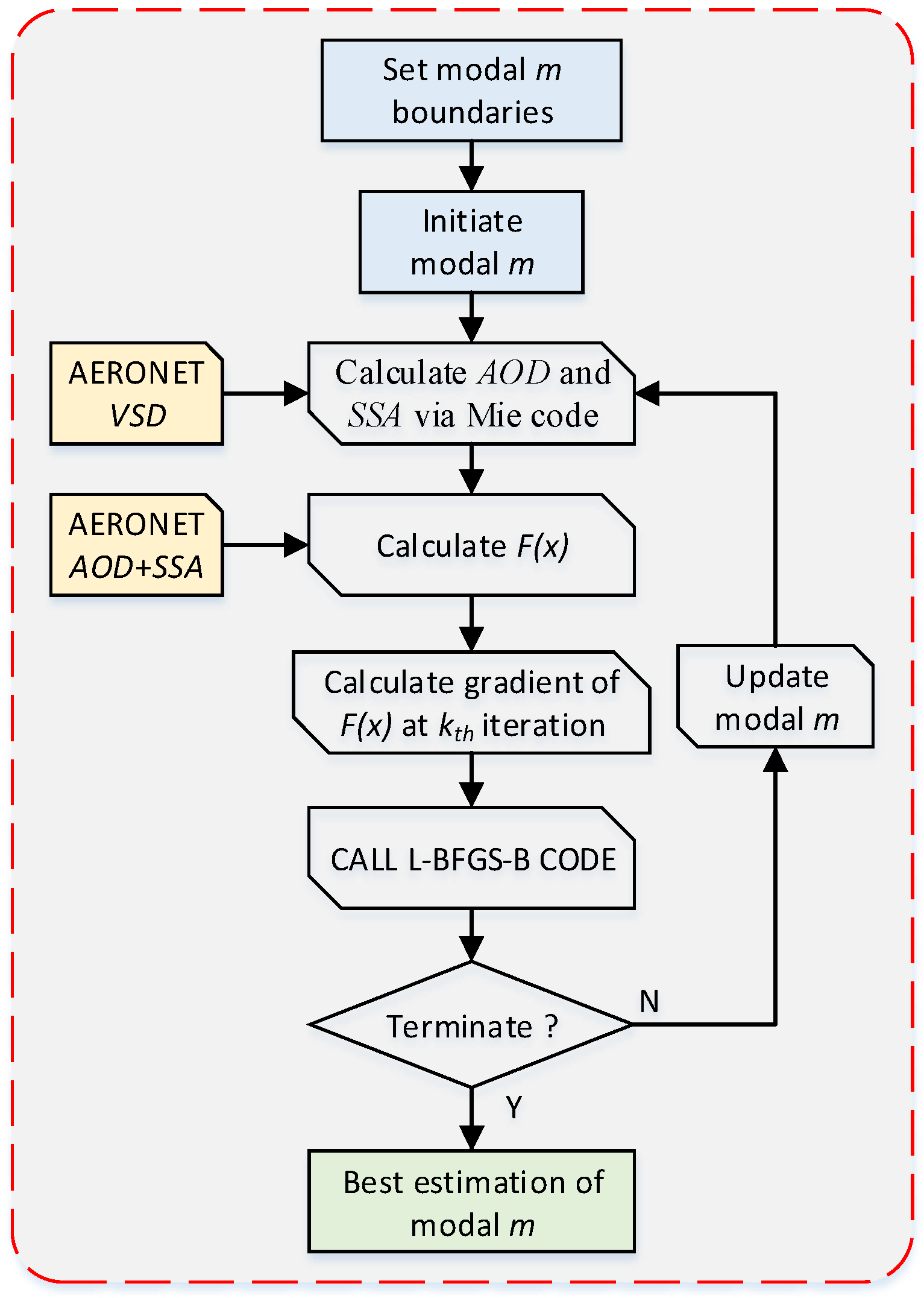
, where epsmch denotes the machine precision and is automatically generated by the code; factor is a user defined parameter and is selected to terminate the run when the change in F(x) is sufficiently small. We chose f a c t o r = 10 7 for moderate accuracy.
  • p r o j   g pgtol , where pgtol was set to a default value of 10−4.
  • No further progress can be made during the line search. When the line search program fails to find a point with an acceptably low objective value after twenty iterations of calculating F(x) or along the steepest descent direction, the calculation terminates. Further details regarding the algorithm and code can be found in the work of Zhu et al. [40].

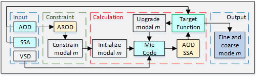
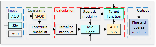
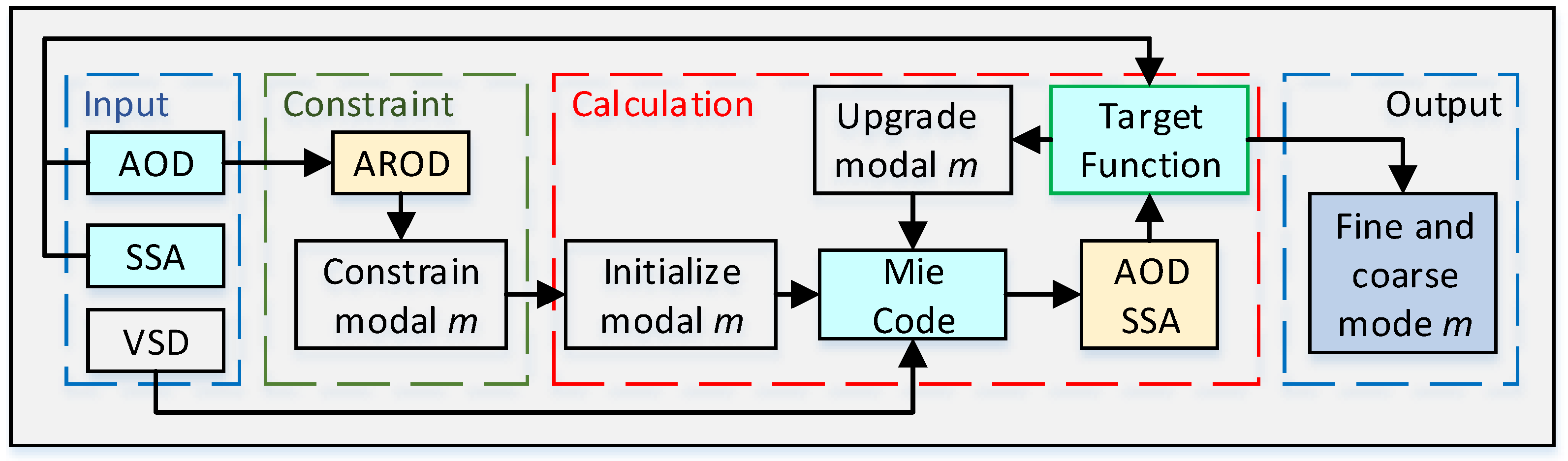
2.6. Process for Inferring Modal m Values

Figure 2 shows a flow diagram of the process for estimating the modal m values, where each step in this process is summarized as follows:
  • Setting the modal m boundaries: 1.33 n f 1.53 , 0.0005 k f 0.1 , 1.50 n C 1.60 , and 0.0005 k C , 0.44 0.015 [12,32].
  • Initiating modal m values: n f = 1.35 , k f = 0.01 , n C = 1.55 , and k C , 0.44 = k C , 0.67 1.02 = 0.001 .
  • Calculating spectral AOD and SSA using Mie theory and AERONET VSD information. Consistent with AERONET, AOD and SSA are calculated in 22 logarithmically spaced particle-size bins over the range of 0.05–15 µm, where Equations (4)–(6) can be expressed in the following form:
    AOD λ ( x ) = f 3 Q e x t , f , i ( x ) 4 r i V f ( r i ) + C 3 Q e x t , C , i ( x ) 4 r i V C ( r i )
    SAOD λ ( x ) = f 3 Q s c a , f , i ( x ) 4 r i V f ( r i ) + C 3 Q s c a , C , i ( x ) 4 r i V C ( r i )
    SSA = AOD ( x ) SAOD ( x )
    where AODλ and SAODλ are the estimated AOD and SAOD resulting from scattering effects at wavelength λ; ri denotes the radius of the ith particle size bin; V(ri) is the volume within the ith particle size bin; Qext,i(x) and Qsca,i(x) are the attenuation and scattering factors, respectively, from Mie theory at ri; and x = ( n f , k f , n c , k c , 0.44 ) represents the modal refractive index vector to be retrieved, where the subscripts f and c represent the fine- and coarse-mode aerosols, respectively.
  • Calculating the value of F(x) based on Equation (10).
  • Calculating the gradient of F(x) under the current iteration k with x k = ( n f , k f , n C , k C , 0.44 ) k .
  • Calling the L-BGRS-B code to search for probable solutions.
  • Checking whether the output from step 6 meets the termination requirements. If so, the best estimations of the modal m values are exported; if not, the modal m values are updated and the loop is repeated.

3. Numerical Tests

3.1. Aerosol Models

The aerosol models used in the current study were based on the summary of aerosol properties provided by Dubovik et al. [12] and those determined in our previous study [35]. We chose four typical aerosol models, including biomass burning (BB), urban industry (UI), sub-continental (SC), and desert dust (DD) aerosol models for performing numerical tests. The basic models of BB, UI, SC, and DD were from long-term observations conducted at the AERONET sites named Mongu, GSFC, INDOX, and Solar Village, respectively [12,32]. Considering the goal of inferring modal m values, we modified the m values for fine- and coarse-mode particles. Specifically, the fine-mode m for BB was set to 1.47 + 0.02 i , while the coarse mode was replaced by dust aerosols [12,32]. Considering that fine particles were dominant and coarse dust aerosols may be related to pollution, the k values were assumed to be wavelength independent with a value of 1.55 + 0.003 i . Similarly, the m values of fine and coarse aerosols for UI were set to 1.41 + 0.003 i and 1.55 + 0.003 i , respectively [12,32]. In the case of SC, the fine-mode m was set to 1.44 + 0.01 i ; due to the high dust particle volume indicated by the absorption characteristics, the coarse-mode m values were set to 1.55 + 0.003 i at 0.44 μm and 1.55 + 0.0015 i for 0.67–1.02 μm [12,32]. Finally, in the case of DD, the m of the fine-mode aerosols was 1.47 + 0.02 i , where the m values of the coarse-mode aerosols were 1.55 + 0.004 i at 0.44 μm and 1.55 + 0.002 i for 0.67–1.02 μm [12,32].
Table 2 shows details of the inputs used in the aerosol models in this study, including modal m values, VSD, and spectral variations of AOD and SSA [12,32]. All the aerosol models follow a bimodal lognormal function for particle size distribution. C, R, and D donate the particle volume concentration, median radius, and standard deviation, respectively. It should be noted that the AOD values at 0.44 μm of the four aerosol models were all set to 0.5 in order to fully consider the effect of the random error of VSD and spectral AOD and SSA on inferring modal m values.

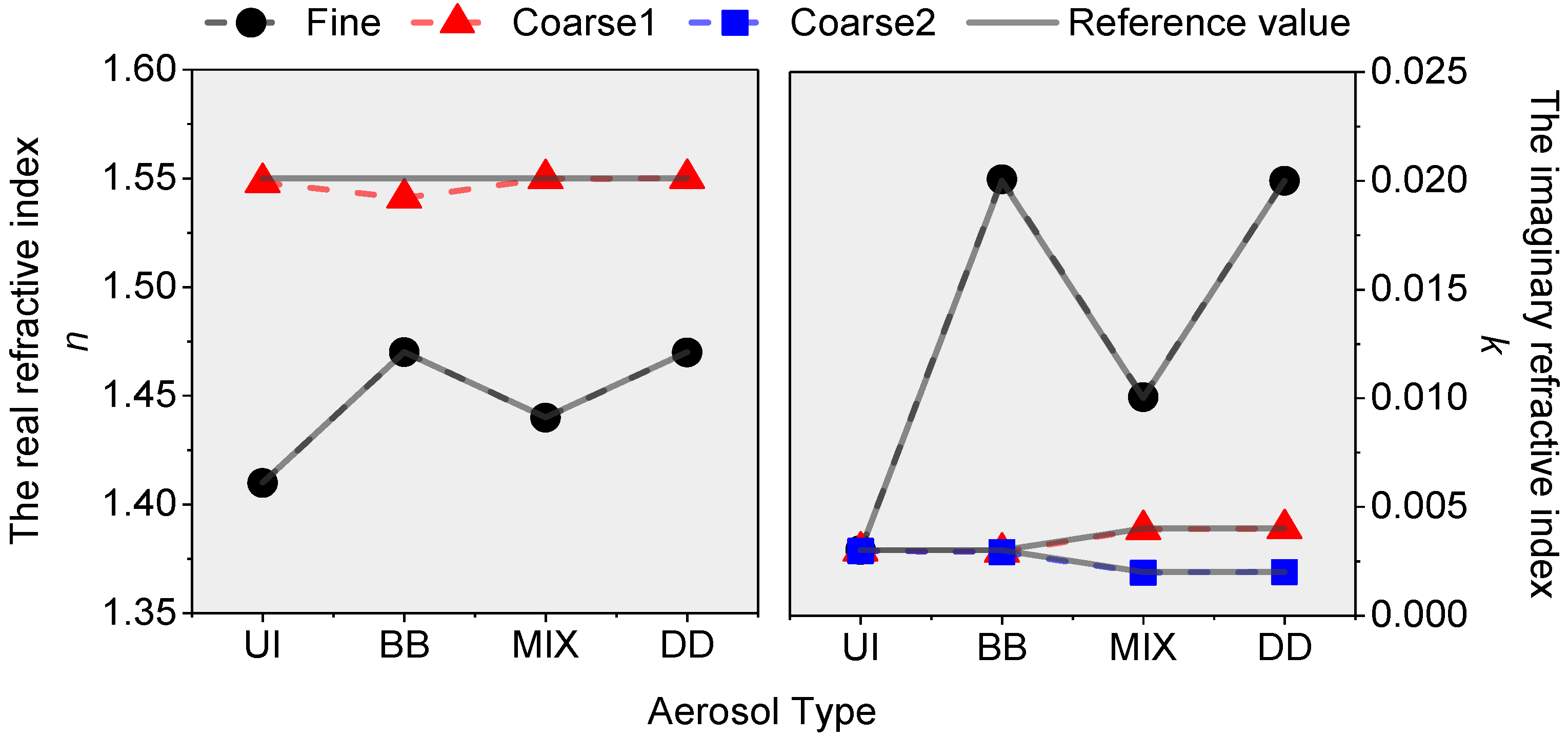
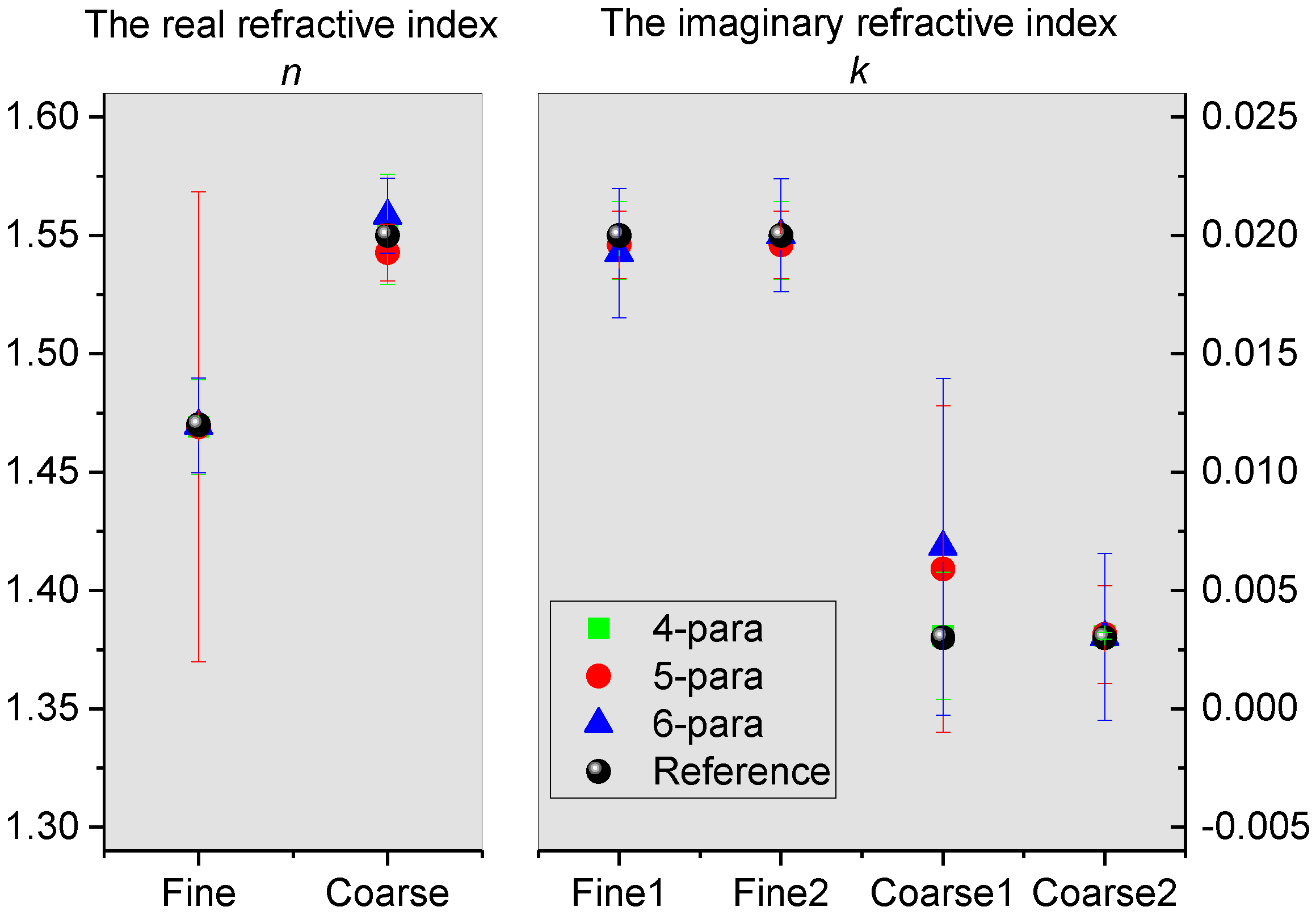
3.2. Self-Consistency Analysis

In this section, we analyze the performance of the proposed modal m inversion scheme under error free conditions. Specifically, the typical aerosol AOD, SSA, and VSD data shown in Table 2 were set as inputs without introducing any random noise; then, the best estimation of modal m values was obtained using the inferring process. Figure 3 shows the results of the self-consistency analysis. In general, fine- and coarse-mode m values under different assumptions of the aerosol type were successfully retrieved in the case where no errors were introduced in the input parameters. It can be seen that the maximum deviations of estimated n and k from the inputs were both observed for the BB aerosol model. The reference values of n and k were 1.55 and 0.003, respectively, while the estimated n and k values were 1.54 and 0.0029, corresponding to maximum deviations of around 0.58% and 2.87%, respectively. A similar result was observed in the study of Zhang et al. [3], where under BB aerosol conditions, the relative deviation of the estimated n and k values reached a maximum of 3% and 35%, respectively. This may be due to the optical contribution of coarse-mode aerosols in BB, the aerosol model being too weak to obtain a reasonable estimation of coarse-mode m values.

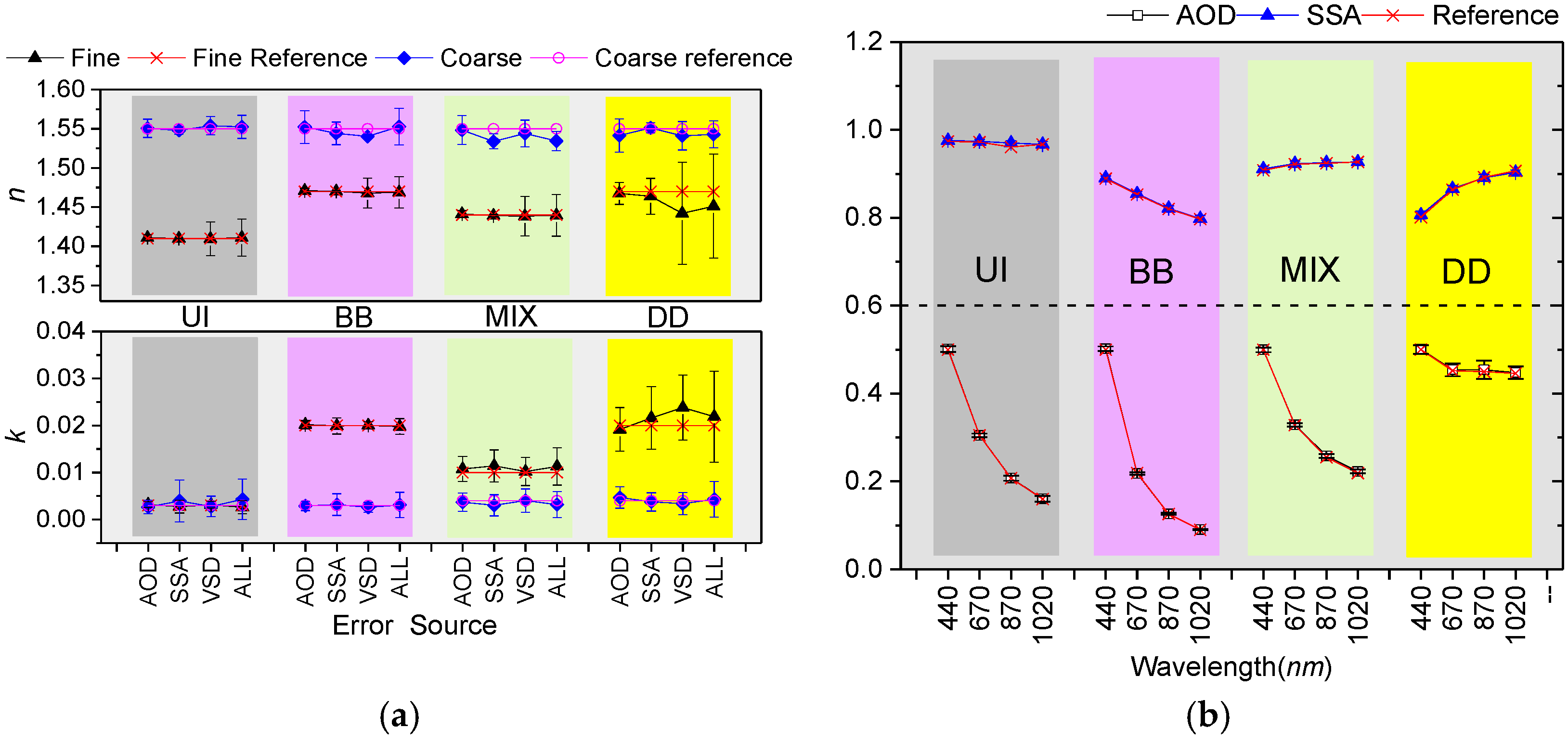
3.3. Simulation of Input Errors

The effect of AOD, SSA, VSD, and their synergetic errors on the estimation of modal m values is discussed in this section. Here, we introduced random noise (with a normal distribution) on the AOD, SSA, and VSD values. The maximum random noise values for AOD, SSA, and VSD were 0.02, 0.03, and 35% in 22 particle-size bins according to the uncertainty estimation for AERONET inversion products described in Section 2.1 [12,23]. The estimated modal m values of each aerosol model were the average of twenty calculations with random noise.
Figure 4a compares the estimated modal m values under different error conditions with the reference m values. In general, the estimated modal m values were similar to the reference values. With the introduction of a single error source (ΔAOD, ΔSSA, or ΔVSD), the estimation error of the modal m values was quite small for the UI aerosol model data, while ΔVSD resulted in a relatively small error (about 0.006) in coarse-mode n values for the BB aerosol model. For the MIX aerosol model, ΔSSA noise resulted in large errors of 0.016 in both the coarse-mode n and fine-mode k values, while for the DD aerosol model, ΔVSD resulted in the largest biases in estimating fine-mode m values (3.4% for n and 25% for k). Considering synergetic errors where all error sources were added (ALL in Figure 4), obvious deviations were observed when estimating fine-mode m values in DD aerosol models. This is because the contribution to AOD from fine-mode particles is very small for DD-type aerosol; therefore, the accuracy of fine-mode m values is sacrificed to compensate for the input errors. The mean deviations were 0.32% ± 0.64% and 0.28% ± 0.56% for fine- and coarse-mode n values and 2.11% ± 11.59% and 8.4% ± 26.42% for fine- and coarse-mode k values for the averages of twenty calculations.
As the ultimate goal of inferring modal aerosol refractive indices retrieval is to generate reliable values for atmospheric radiative transfer modelling, retrieving an incorrect modal refractive index will more or less influence the modelling accuracy. To illustrate how far off the bias will reach, we recovered the spectral AOD and SSA in the presence of synergetic errors, because AOD and SSA are two key parameters to simulate the light extinction and scattering effects caused by aerosol particles in modern atmospheric radiative transfer models. Figure 4b shows the recovery of spectral AOD and SSA using the estimated modal m values and the comparison with the reference values listed in Table 2. Generally, the spectral AOD and SSA are in good agreement with the reference values. The absolute error of AOD at 870 nm in DD type (0.024) and SSA at 0.67 μm in UI type (0.014) are the largest but still acceptable in many situations, for the uncertainty of widely used AERONET inversed AOD and SSA are around 0.02 and 0.03, respectively.
In the presence of synergetic errors, our estimation method slightly overestimates modal n values, while it underestimates k. However, our method was able to not only clearly distinguish fine- and coarse-mode m values but also rebuild the spectral AOD and SSA within the uncertainty of AERONET products.

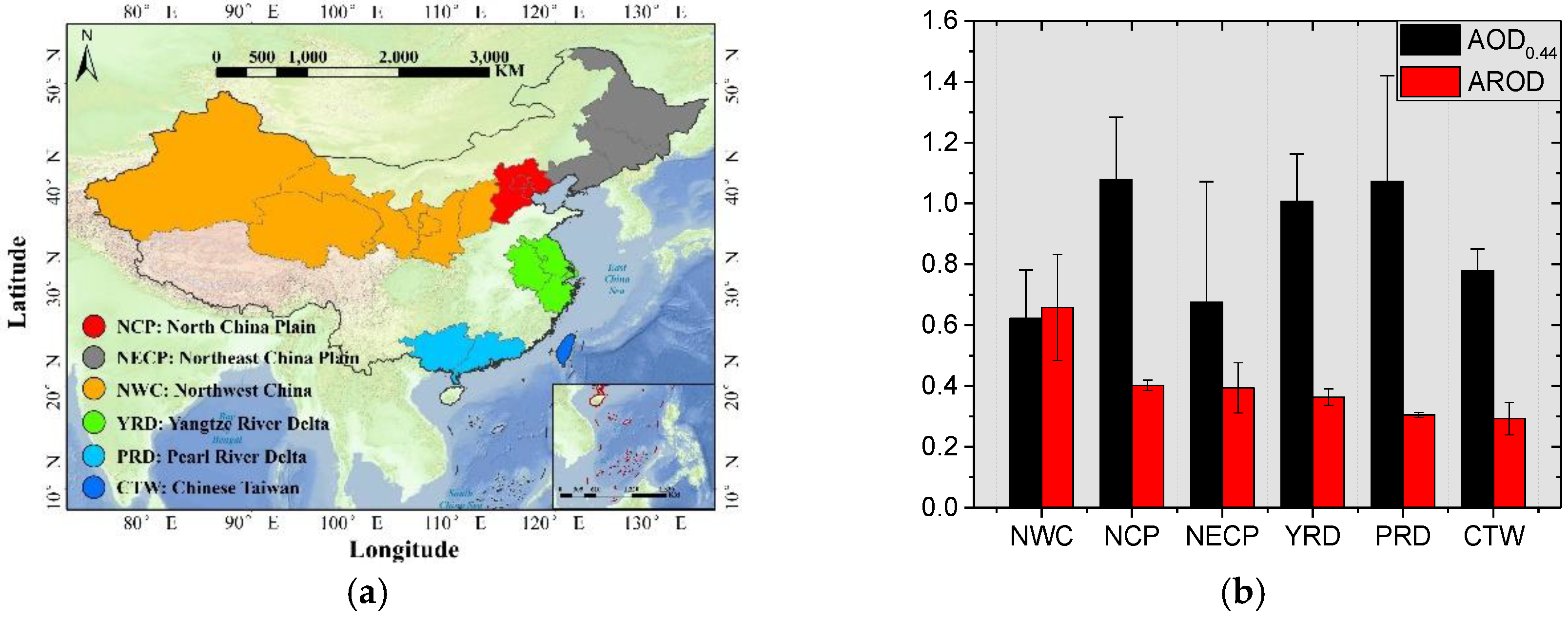
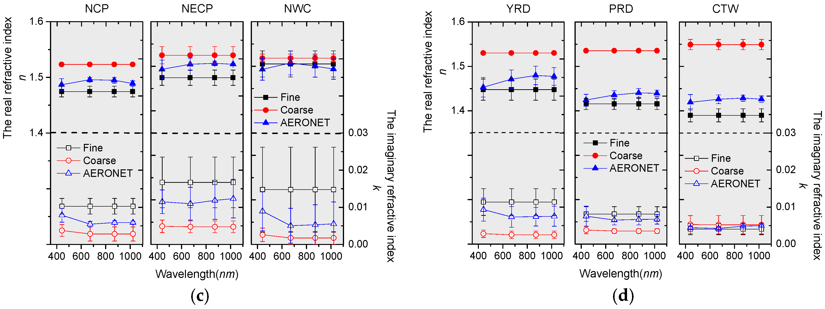
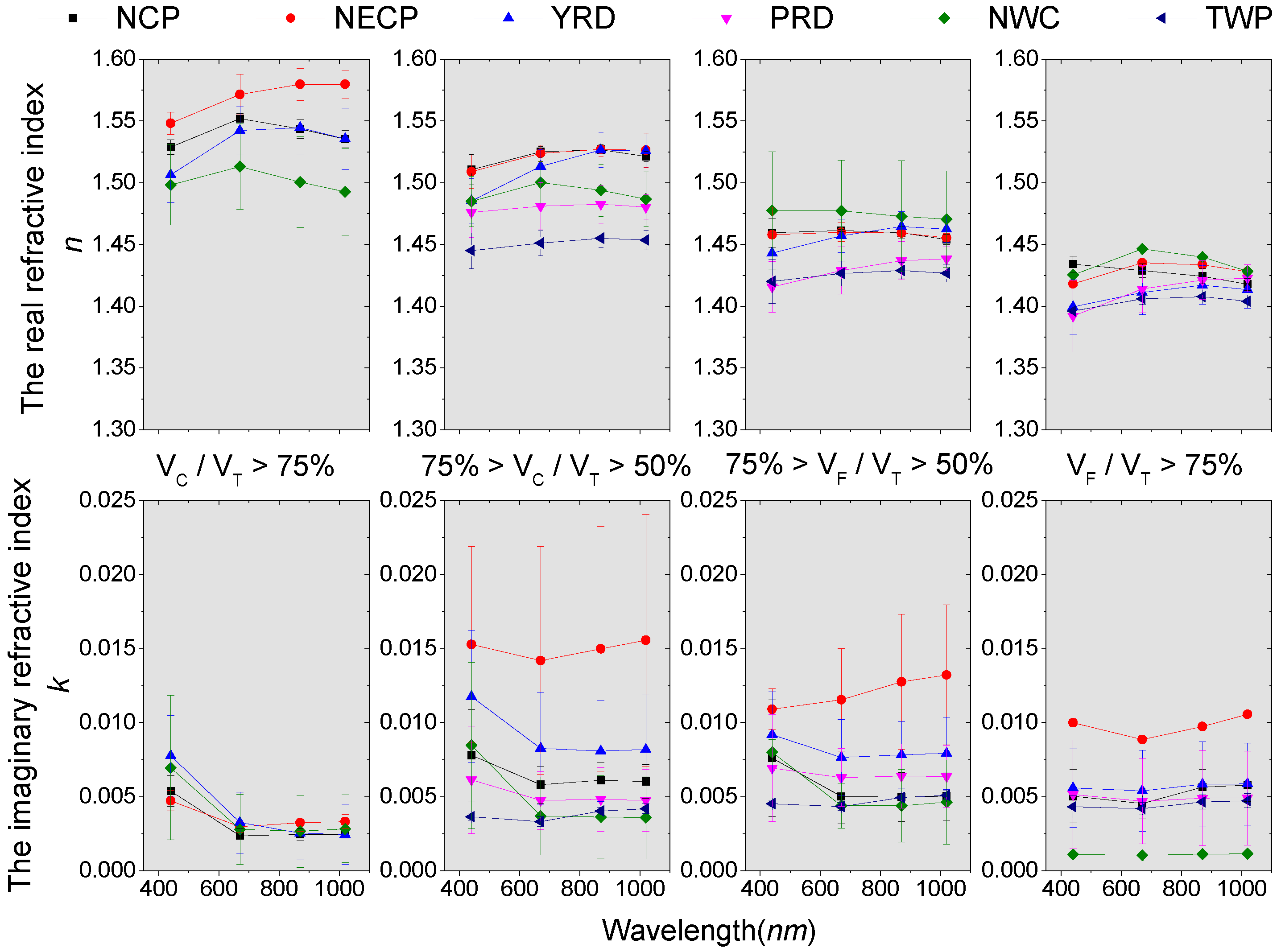
4. Modal Refractive Indices in Typical Regions of China

The modal refractive index inferring scheme was applied to the AERONET inversion products from the sites listed in Table 1. Figure 5a shows the geographical information of six typical regions over China, including North China Plain (NCP), Northeast China Plain (NECP), Northwest China (NWC), Yangtze River Delta (YRD), Pearl River Delta (PRD), and Chinese Taiwan (CTW). The western part of China is characterized by desert, sandy weather, and sparse population, while the eastern part is mostly plains and hills with abundant rainfall, dense population, and advanced industry [41]. Such distinct geographical features result in specific aerosol characteristics; for example, western China is dominated by continental and desert dust aerosol, while the eastern part generally has urban industry aerosol [42,43].
Figure 5b shows a histogram of the annual mean AOD0.44 and AROD values from the six typical regions in China. The AOD0.44 values in NCP, YRD, and PRD were larger than 1.0, indicating a high aerosol load over these industrialized regions, while the NECP and CTW regions showed annual mean AOD0.44 values of 0.7–0.8, with NWC showing the lowest value. Considering the regional differences in AROD values, we conclude that aerosols in the NWC region mainly originated from coarse-mode dust particles, while those in other regions were mainly anthropogenic aerosols (AROD < 0.4) [35].
Figure 5c,d show variations in the m products from AERONET and estimated modal m values as a function of wavelength. Generally, coarse-mode n values were higher (and fine-mode values were lower) than the AERONET products. This was attributed to the coarse-mode dust particles strongly scattering light, resulting in higher k values [4]. The fine-mode k values were higher than those of the AERONET products while those of the coarse mode were lower; fine particles are mainly emitted from human activities and consist of many light-absorbing components, resulting in higher k values [14,44]. The minerals forming the dust particles generally have moderate absorption characteristics at 0.44 μm and weak absorption between 0.67 μm and 1.02 μm; thus, the coarse-mode k was much lower than the fine-mode values [12,25].
The annual mean m values across China were ( 1.45 ± 0.04 ) + ( 0.0109 ± 0.0046 ) i for fine mode and ( 1.53 ± 0.01 ) + ( 0.0039 ± 0.0011 ) i ( 0.0034 i ± 0.0013 i at 0.44 μm) for coarse mode aerosols. In the regions with low AROD values (e.g., PRD and CTW), the fine-mode m values were closer to the AERONET products, suggesting that these areas mainly contained fine-mode particles. However, in high-AROD (AROD > 0.6) regions such as NWC, AERONET m products were closer to the coarse-mode m values, indicating coarse-mode aerosols dominated this region. These results indicate that our estimation results are generally reliable, and the assumptions within our modal m inferring method are consistent with the characteristics of the actual aerosols.
The modal m values showed distinct regional differences. The coarse-mode n values of the six regions were all in the range of 1.52 to 1.56. The fine-mode n values in the NWC, NCP, NECP, YRD, PRD, and CTW regions were 1.51 ± 0.03, 1.47 ± 0.01, 1.47 ± 0.02, 1.45 ± 0.02, 1.41 ± 0.01, and 1.39 ± 0.01, respectively, showing a decrease from the northwest to the southeast. The annual mean kf,0.44 values in the NWC, NCP, NECP, and YRD regions were >0.01, while those of PRD and CTW were <0.01 and <0.005, respectively. This was mainly due to the CTW region being influenced by maritime aerosol, where the proportion of water-soluble components in CTW was higher than in other areas, resulting in a low k of the dominant fine-mode aerosols as k values of water-soluble particles are typically 1.40 + 0.003 i [12,42]. In contrast to CTW, NECP, NCP, and YRD were characterized by UI aerosols, where the suspended anthropogenic aerosols resulted in high fine-mode k values [43,45].
In addition, it was observed that the differences between fine- and coarse-mode n values were small in the northern part of China (NWC, NCP, and NECP), but large in the southern part of China (YRD, PRD, and CTW). On the contrary, the differences between modal k values were large in the north, but small in the south. This indicates that northern China suffers more dust events than the south, and the aerosol compositions in the north are labile, while they are much more stable in the south.

5. Discussion

5.1. Constraint of Aerosol Complex Refractive Indices

To calculate the modal m values from AERONET LV2.0 inversion products, the following four parameters were solved: the wavelength-independent nf, kf, and nc values, along with k C , 0.44 . The kc values at 0.67, 0.87, and 1.02 μm were equal. When AROD > 0.4, k C , 0.44 = 2 k C , 0.67 1.02 , while when AROD < 0.4, we set k C , 0.44 = k C , 0.67 1.02 . Here are two reasons to make such constraint.
Using wavelength-independent modal m values is considered reliable as they compared well with worldwide AERONET observations. Dubovik et al. [12] observed that m values at sites dominated by fine-mode particles were generally wavelength independent, while n values at sites dominated by coarse dust particles varies little between 0.44 and 1.02 μm [46,47,48]. However, k values measured at 0.44 μm for areas dominated by coarse particles were double those at 0.67, 0.87, and 1.02 μm. To further validate the constraint of wavelength-independent modal m values, we analyzed the annual mean m variations with increasing wavelengths under different volume ratios of fine and coarse particles from the 21 AERONET sites over China. Figure 6 shows that the n values varied little (<1.5%) between 0.44 and 1.02 μm for both fine-dominant ( V F / V T > 75 % ) and coarse-dominant ( V C / V T > 75 % ) cases, which supports the assumption of wavelength-independent n values for both fine and coarse particles. The k values under fine-dominant cases were generally wavelength independent, while the coarse-dominant cases showed distinct variations in different regions (maximum at 0.44 μm, then decreased by more than half between 0.67 and 1.02 μm). Such results suggest that the use of wavelength-independent modal m value settings is reasonable.
The use of wavelength-independent modal m values reduces the number of parameters to be inferred, which results in more accurate estimations when input errors exist. There are only eight constraints (spectral AOD and SSA at 0.44, 0.67, 0.87, and 1.02 μm) used to infer modal m values, which all contain finite errors in most cases [3,23]. In general, it is quite difficult to ensure accurate results when errors are present in limited constraints. Hence, we considered different parameters, i.e., x = ( n f , k f , n c , k c , 0.44 ) , x = ( n f , k f , n c , k c , 0.44 , k c , 0.67 1.02 ) , and x = ( n f , k f , 0.44 , k f , 0.67 1.02 , n c , k c , 0.44 , k c , 0.67 1.02 ) . Figure 7 compares the retrieval results for these conditions with the reference value obtained under random error conditions. The aerosol model used to produce the data shown in Figure 7 is described in Section 3.1, where the estimated modal m values are the average of twenty estimation results with normal distribution errors of AOD, SSA, and VSD applied simultaneously. It is clear that the use of fewer parameters produced more accurate results, whereby the results of the setting with four parameters (4-para) were closest to the reference value, while the 6-para setting resulted in the largest deviations, especially for the coarse-mode m values. As a result, the wavelength-independent setting of modal m values was adopted here to ensure both the rationality of modal m properties and the accuracy of the inferring results.

5.2. Rationality of the Use of VSD

As initial products, AERONET m and VSD are inherently linked. The use of VSD in our inferring process will make the estimated modal m a function of AERONET m. Such an inherent linkage or functional relationship may cause the estimated modal m to be an artefact of the presented method. Thus, it is necessary to discuss whether or not the use of VSD is rational.
Seeing the non-linear nature of the forward model and amount of a priori constraints (e.g., constraining the solution by a priori estimates and smoothness constraints of the solution) used in AERONET inversion strategies, the influence of m on retrieving VSD may be not as strong as we expected. On the one hand, Dubovik and King [23] found that the retrieval of VSD can be more stable when both VSD and m were retrieved than when m is fixed to assumed values and only VSD was retrieved. They explained that when m is fixed, only the VSD can be changed and compensated for all the observation noise, while if both VSD and m are retrieved simultaneously, the noise will only be partially tied in VSD. According to their numerical test results, it is obvious that whether m is fixed or not, will not make much difference to the retrieval of VSD, and the retrieval of VSD fits well with the reference values in different cases. Thus, the retrieval of VSD is less influenced by the setting of m. On the other hand, Xu et al. [31] developed a new method to retrieve aerosol microphysical properties using photo-polarimetric measurements, which follows the same AERONET inversion strategies but a different assumption of mode-dependent refractive index. In their case studies, VSD and m were retrieved simultaneously from their new inversions and AERONET inversions, and in general, their retrievals of VSD agree quite well with the AERONET inversions. It can be inferred from the agreement that the retrieval of VSD depends less on refractive index assumptions, and at the same time, it has proven to be a good description of the real aerosol state from previous studies [49,50,51,52]. Therefore, the linkage between the setting of RI and VSD is generally weak, and the use of VSD in our inferring scheme is reasonable.
To think of it another way, the AERONET inversion algorithm couples the modal aerosol refractive indices into one parameter, and our inferring method decouples the modal aerosol refractive indices from the AERONET m values. The AERONET inversion algorithm gives us the combination of m and VSD to best fit the observed direct sun and diffuse sky radiance. As the retrieval of VSD saves the information of the actual aerosol size distribution, the m must have preserved the information of modal aerosol refractive indices. Thus, the functional relationship between the estimated modal m and AERONET m is in fact a functional relationship between the real aerosol refractive index and the estimated modal m. Therefore, our estimation of modal aerosol refractive indices is not an artefact but a reasonable inference.
In addition, the results of the numerical tests also support the use of VSD. As described in Section 3.3, original AOD, SSA, and VSD are modified by their expected errors and assumed to be the “AERONET inversion products”, then these “AERONET inversion products” were introduced into the inferring process to obtain an estimation of modal m values. According to the comparisons between estimated and reference modal m value, the use of assumed “AERONET inversion products” VSD in our inferring scheme works generally well in regaining the reference modal m values and in recovering the original AOD and SSA. In addition, the modal m values estimated from different AERONET observations in Section 4 are in good agreement with our current knowledge. Thus, the use of VSD is reasonably satisfactory, and at least for now, the presented method is as good as it gets.

6. Conclusions

The goal of the presented study was to infer complex refractive indices of fine- and coarse-mode aerosols from AERONET inversion products. The finite constraints of spectral AOD and SSA with noise required pretreatment of the modal m values, where the use of typical aerosol models allowed us to test and evaluate our modal m inferring method. Numerical tests showed that in the presence of synergetic noise in AOD, SSA, and VSD data, the proposed inferring scheme slightly overestimated fine- and coarse-mode n values but underestimated k values by 2.11% ± 11.59% for fine-mode aerosols and by 8.4% ± 26.42% for coarse-mode aerosols. Furthermore, our method was applied to the 21 AERONET dataset to investigate the regional properties of fine- and coarse-mode m values over China. We found that annual mean coarse-mode n and k values ranged from 1.52 to 1.56 and from 0.002 to 0.006, respectively. The fine-mode n values decreased from the northwest (1.51 ± 0.03) to the southeast (1.39 ± 0.01), while the fine-mode k values were generally larger than 0.008 across China.
We hope this study helps compensate for the lack of modal aerosol refractive index estimations, which cannot be obtained from AERONET products, and improves our understanding of the different roles of fine- and coarse-mode aerosols in the Earth-Ocean-Atmosphere system.

Author Contributions

Conceptualization, Q.-X.C.; methodology, Q.-X.C.; validation, Y.Y.; formal analysis, Q.-X.C.; investigation, M.X.; data curation, W.-X.S.; writing—original draft preparation, Q.-X.C.; writing—review and editing, Q.-X.C.; visualization, W.-X.S.; supervision, Y.Y.; project administration, H.-P.T.; funding acquisition, M.X. and Y.Y.

Funding

This research was funded by the National Natural Science Foundation of China, grant numbers 51776051 and 51436009.

Acknowledgments

The authors would like to thank AERONET for kindly providing the inversion data. In addition, a very special acknowledgement is made to the editors and referees who provided important comments that improved this paper.

Conflicts of Interest

The authors declare no conflict of interest.

References

  1. Ealo, M.; Alastuey, A.; Perez, N.; Ripoll, A.; Querol, X.; Pandolfi, M. Impact of aerosol particle sources on optical properties in urban, regional and remote areas in the north-western mediterranean. Atmos. Chem. Phys. 2018, 18, 1149–1169. [Google Scholar] [CrossRef]
  2. Chen, Q.-X.; Shen, W.-X.; Yuan, Y.; Tan, H.-P. Verification of aerosol classification methods through satellite and ground-based measurements over harbin, northeast china. Atmos. Res. 2019, 216, 167–175. [Google Scholar] [CrossRef]
  3. Zhang, Y.; Li, Z.Q.; Zhang, Y.H.; Li, D.H.; Qie, L.L.; Che, H.Z.; Xu, H. Estimation of aerosol complex refractive indices for both fine and coarse modes simultaneously based on aeronet remote sensing products. Atmos. Meas. Tech. 2017, 10, 3203–3213. [Google Scholar] [CrossRef]
  4. Bran, S.H.; Jose, S.; Srivastava, R. Investigation of optical and radiative properties of aerosols during an intense dust storm: A regional climate modeling approach. J. Atmos. Sol.-Terr. Phy. 2018, 168, 21–31. [Google Scholar] [CrossRef]
  5. Mallet, M.; Solmon, F.; Roblou, L.; Peers, F.; Turquety, S.; Waquet, F.; Jethva, H.; Torres, O. Simulation of optical properties and direct and indirect radiative effects of smoke aerosols over marine stratocumulus clouds during summer 2008 in california with the regional climate model regcm. J. Geophys. Res.-Atmos. 2017, 122, 10288–10313. [Google Scholar] [CrossRef]
  6. Chen, Q.; Yuan, Y.; Huang, X.; He, Z.; Tan, H. Assessment of column aerosol optical properties using ground-based sun-photometer at urban Harbin, Northeast China. J. Environ. Sci. China 2018, 74, 50–57. [Google Scholar] [CrossRef]
  7. Nakayama, T.; Sato, K.; Imamura, T.; Matsumi, Y. Effect of oxidation process on complex refractive index of secondary organic aerosol generated from isoprene. Environ. Sci. Technol. 2018, 52, 2566–2574. [Google Scholar] [CrossRef] [PubMed]
  8. Rafferty, A.; Preston, T.C. Measuring the size and complex refractive index of an aqueous aerosol particle using electromagnetic heating and cavity-enhanced raman scattering. Phys. Chem. Chem. Phys. 2018, 20, 17038–17047. [Google Scholar] [CrossRef] [PubMed]
  9. Liu, P.F.; Zhang, Y.; Martin, S.T. Complex refractive indices of thin films of secondary organic materials by spectroscopic ellipsometry from 220 to 1200 nm. Environ. Sci. Technol. 2013, 47, 13594–13601. [Google Scholar] [CrossRef] [PubMed]
  10. Marley, N.A.; Gaffney, J.S.; Baird, C.; Blazer, C.A.; Drayton, P.J.; Frederick, J.E. An empirical method for the determination of the complex refractive index of size-fractionated atmospheric aerosols for radiative transfer calculations. Aerosol. Sci. Technol. 2001, 34, 535–549. [Google Scholar] [CrossRef]
  11. Shepherd, R.H.; King, M.D.; Marks, A.A.; Brough, N.; Ward, A.D. Determination of the refractive index of insoluble organic extracts from atmospheric aerosol over the visible wavelength range using optical tweezers. Atmos. Chem. Phys. 2018, 18, 5235–5252. [Google Scholar] [CrossRef] [Green Version]
  12. Dubovik, O.; Holben, B.; Eck, T.F.; Smirnov, A.; Kaufman, Y.J.; King, M.D.; Tanre, D.; Slutsker, I. Variability of absorption and optical properties of key aerosol types observed in worldwide locations. J. Atmos. Sci. 2002, 59, 590–608. [Google Scholar] [CrossRef]
  13. Gong, C.S.; Xin, J.Y.; Wang, S.G.; Wang, Y.S.; Zhang, T.J. Anthropogenic aerosol optical and radiative properties in the typical urban/suburban regions in china. Atmos. Res. 2017, 197, 177–187. [Google Scholar] [CrossRef]
  14. Tuet, W.Y.; Chen, Y.L.; Xu, L.; Fok, S.; Gao, D.; Weber, R.J.; Ng, N.L. Chemical oxidative potential of secondary organic aerosol (soa) generated from the photooxidation of biogenic and anthropogenic volatile organic compounds. Atmos. Chem. Phys. 2017, 17, 839–853. [Google Scholar] [CrossRef]
  15. Mao, Q.J. Recent developments in geometrical configurations of thermal energy storage for concentrating solar power plant. Renew. Sustain. Energy Rev. 2016, 59, 320–327. [Google Scholar] [CrossRef]
  16. Mao, Q.J.; Chen, H.Z.; Zhao, Y.Z.; Wu, H.J. A novel heat transfer model of a phase change material using in solar power plant. Appl. Therm. Eng. 2018, 129, 557–563. [Google Scholar] [CrossRef]
  17. Hu, W.; Niu, H.Y.; Zhang, D.Z.; Wu, Z.J.; Chen, C.; Wu, Y.S.; Shang, D.J.; Hu, M. Insights into a dust event transported through Beijing in spring 2012: Morphology, chemical composition and impact on surface aerosols. Sci. Total Environ. 2016, 565, 287–298. [Google Scholar] [CrossRef] [PubMed]
  18. Wang, G.H.; Cheng, C.L.; Huang, Y.; Tao, J.; Ren, Y.Q.; Wu, F.; Meng, J.J.; Li, J.J.; Cheng, Y.T.; Cao, J.J.; et al. Evolution of aerosol chemistry in Xi’an, Inland China, during the dust storm period of 2013—Part 1: Sources, chemical forms and formation mechanisms of nitrate and sulfate. Atmos. Chem. Phys. 2014, 14, 11571–11585. [Google Scholar] [CrossRef]
  19. Mishchenko, M.I.; Cairns, B.; Kopp, G.; Schueler, C.F.; Fafaul, B.A.; Hansen, J.E.; Hooker, R.J.; Itchkawich, T.; Maring, H.B.; Travis, L.D. Accurate monitoring of terrestrial aerosols and total solar irradiance—Introducing the glory mission. B Am. Meteorol. Soc. 2007, 88, 677. [Google Scholar] [CrossRef]
  20. Hasekamp, O.P.; Litvinov, P.; Butz, A. Aerosol properties over the ocean from parasol multiangle photopolarimetric measurements. J. Geophys. Res.-Atmos. 2011, 116. [Google Scholar] [CrossRef]
  21. Woo, C.G.; You, S.; Lee, J. Determination of refractive index for absorbing spheres. Optik 2013, 124, 5254–5258. [Google Scholar] [CrossRef]
  22. Patterson, E.M.; Gillette, D.A.; Stockton, B.H. Complex index of refraction between 300 and 700 nm for saharan aerosols. J. Geophys. Res.-Atmos. 1977, 82, 3153–3160. [Google Scholar] [CrossRef]
  23. Dubovik, O.; King, M.D. A flexible inversion algorithm for retrieval of aerosol optical properties from sun and sky radiance measurements. J. Geophys. Res.-Atmos. 2000, 105, 20673–20696. [Google Scholar] [CrossRef]
  24. Nakajima, T.; Tonna, G.; Rao, R.Z.; Boi, P.; Kaufman, Y.; Holben, B. Use of sky brightness measurements from ground for remote sensing of particulate polydispersions. Appl. Opt. 1996, 35, 2672–2686. [Google Scholar] [CrossRef] [PubMed]
  25. Fedarenka, A.; Dubovik, O.; Goloub, P.; Li, Z.Q.; Lapyonok, T.; Litvinov, P.; Barel, L.; Gonzalez, L.; Podvin, T.; Crozel, D. Utilization of aeronet polarimetric measurements for improving retrieval of aerosol microphysics: Gsfc, beijing and dakar data analysis. J. Quant. Spectrosc. Radiat. Transf. 2016, 179, 72–97. [Google Scholar] [CrossRef]
  26. He, Z.Z.; Mao, J.K.; Han, X.S. Non-parametric estimation of particle size distribution from spectral extinction data with pca approach. Powder Technol. 2018, 325, 510–518. [Google Scholar] [CrossRef]
  27. He, Z.Z.; Qi, H.; Yao, Y.C.; Ruan, L.M. Inverse estimation of the particle size distribution using the fruit fly optimization algorithm. Appl. Therm. Eng. 2015, 88, 306–314. [Google Scholar] [CrossRef]
  28. Danylevsky, V.; Ivchenko, V.; Milinevsky, G.; Sosonkin, M.; Goloub, P.; Li, Z.Q.; Dubovik, O. Atmosphere aerosol properties measured with aeronet/photons sun-photometer over kyiv during 2008–2009. Nato Sci. Peace Secur. 2011, 285–294. [Google Scholar]
  29. Dubovik, O.; Smirnov, A.; Holben, B.N.; King, M.D.; Kaufman, Y.J.; Eck, T.F.; Slutsker, I. Accuracy assessments of aerosol optical properties retrieved from aerosol robotic network (aeronet) sun and sky radiance measurements. J. Geophys Res.-Atmos. 2000, 105, 9791–9806. [Google Scholar] [CrossRef]
  30. Kaufman, Y.J.; Gitelson, A.; Karnieli, A.; Ganor, E.; Fraser, R.S.; Nakajima, T.; Mattoo, S.; Holben, B.N. Size distribution and scattering phase function of aerosol-particles retrieved from sky brightness measurements. J. Geophys. Res.-Atmos. 1994, 99, 10341–10356. [Google Scholar] [CrossRef]
  31. Xu, X.G.; Wang, J.; Zeng, J.; Spurr, R.; Liu, X.; Dubovik, O.; Li, L.; Li, Z.Q.; Mishchenko, M.I.; Siniuk, A.; et al. Retrieval of aerosol microphysical properties from aeronet photopolarimetric measurements: 2. A new research algorithm and case demonstration. J. Geophys. Res.-Atmos. 2015, 120, 7079–7098. [Google Scholar] [CrossRef]
  32. Torres, B.; Dubovik, O.; Fuertes, D.; Schuster, G.; Cachorro, V.E.; Lapyonok, T.; Goloub, P.; Blarel, L.; Barreto, A.; Mallet, M.; et al. Advanced characterisation of aerosol size properties from measurements of spectral optical depth using the grasp algorithm. Atmos. Meas. Tech. 2017, 10, 3743–3781. [Google Scholar] [CrossRef]
  33. Chen, Q.X.; Yuan, Y.; Huang, X.; Jiang, Y.Q.; Tan, H.P. Estimation of surface-level pm2.5 concentration using aerosol optical thickness through aerosol type analysis method. Atmos. Environ. 2017, 159, 26–33. [Google Scholar] [CrossRef]
  34. Yuan, Y.; Shuai, Y.; Li, X.W.; Liu, B.; Tan, H.P. Using a new aerosol relative optical thickness concept to identify aerosol particle species. Atmos. Res. 2014, 150, 1–11. [Google Scholar] [CrossRef]
  35. Chen, Q.X.; Yuan, Y.; Shuai, Y.; Tan, H.P. Graphical aerosol classification method using aerosol relative optical depth. Atmos. Environ. 2016, 135, 84–91. [Google Scholar] [CrossRef]
  36. Lee, S.; Hong, J.; Cho, Y.; Choi, M.; Kim, J.; Park, S.S.; Ahn, J.Y.; Kim, S.K.; Moon, K.J.; Eck, T.F.; et al. Characteristics of classified aerosol types in south korea during the maps-seoul campaign. Aerosol. Air Qual. Res. 2018, 18, 2195–2206. [Google Scholar] [CrossRef]
  37. Mishchenko, M.I.; Yang, P. Far-field lorenz-mie scattering in an absorbing host medium: Theoretical formalism and fortran program. J. Quant. Spectrosc. Radiat. Transf. 2018, 205, 241–252. [Google Scholar] [CrossRef]
  38. Mishchenko, M.I.; Dlugach, J.M.; Lock, J.A.; Yurkin, M.A. Far-field far-field lorenz-mie scattering in an absorbing host medium. Ii: Improved stability of the numerical algorithm. J. Quant. Spectrosc. Radiat. Transf. 2018, 217, 274–277. [Google Scholar] [CrossRef]
  39. Dubovik, O.; Herman, M.; Holdak, A.; Lapyonok, T.; Tanre, D.; Deuze, J.L.; Ducos, F.; Sinyuk, A.; Lopatin, A. Statistically optimized inversion algorithm for enhanced retrieval of aerosol properties from spectral multi-angle polarimetric satellite observations. Atmos. Meas. Tech. 2011, 4, 975–1018. [Google Scholar] [CrossRef] [Green Version]
  40. Zhu, C.Y.; Byrd, R.H.; Lu, P.H.; Nocedal, J. Algorithm 778: L-bfgs-b: Fortran subroutines for large-scale bound-constrained optimization. ACM Trans. Math. Softw. 1997, 23, 550–560. [Google Scholar] [CrossRef]
  41. Yang, X.; Li, Z.Q.; Liu, L.; Zhou, L.J.; Cribb, M.; Zhang, F. Distinct weekly cycles of thunderstorms and a potential connection with aerosol type in china. Geophys. Res. Lett. 2016, 43, 8760–8768. [Google Scholar] [CrossRef]
  42. Che, H.Z.; Zhao, H.J.; Wu, Y.F.; Xia, X.G.; Zhu, J.; Dubovik, O.; Estelles, V.; Ma, Y.J.; Wang, Y.F.; Wang, H.; et al. Application of aerosol optical properties to estimate aerosol type from ground-based remote sensing observation at urban area of northeastern china. J. Atmos. Sol.-Terr. Phy. 2015, 132, 37–47. [Google Scholar] [CrossRef]
  43. Kumar, K.R.; Kang, N.; Yin, Y. Classification of key aerosol types and their frequency distributions based on satellite remote sensing data at an industrially polluted city in the yangtze river delta, china. Int. J. Climatol. 2018, 38, 320–336. [Google Scholar] [CrossRef]
  44. Mao, Q.J.; Huang, C.L.; Zhang, H.X.; Chen, Q.X.; Yuan, Y. Aerosol optical properties and radiative effect under different weather conditions in Harbin, China. Infrared Phys. Technol. 2018, 89, 304–314. [Google Scholar] [CrossRef]
  45. Sun, T.Z.; Che, H.Z.; Qi, B.; Wang, Y.Q.; Dong, Y.S.; Xia, X.G.; Wang, H.; Gui, K.; Zheng, Y.; Zhao, H.J.; et al. Aerosol optical characteristics and their vertical distributions under enhanced haze pollution events: Effect of the regional transport of different aerosol types over eastern china. Atmos. Chem. Phys. 2018, 18, 2949–2971. [Google Scholar] [CrossRef]
  46. Arola, A.; Schuster, G.; Myhre, G.; Kazadzis, S.; Dey, S.; Tripathi, S.N. Inferring absorbing organic carbon content from aeronet data. Atmos. Chem. Phys. 2011, 11, 215–225. [Google Scholar] [CrossRef]
  47. Wang, L.; Li, Z.Q.; Tian, Q.J.; Ma, Y.; Zhang, F.X.; Zhang, Y.; Li, D.H.; Li, K.T.; Li, L. Estimate of aerosol absorbing components of black carbon, brown carbon, and dust from ground-based remote sensing data of sun-sky radiometers. J. Geophys. Res.-Atmos. 2013, 118, 6534–6543. [Google Scholar] [CrossRef] [Green Version]
  48. Zhang, Y.; Li, Z.Q.; Sun, Y.L.; Lv, Y.; Xie, Y.S. Estimation of atmospheric columnar organic matter (om) mass concentration from remote sensing measurements of aerosol spectral refractive. Atmos. Environ. 2018, 179, 107–117. [Google Scholar] [CrossRef]
  49. Holben, B.N.; Kim, J.; Sano, I.; Mukai, S.; Eck, T.F.; Giles, D.M.; Schafer, J.S.; Sinyuk, A.; Slutsker, I.; Smirnov, A.; et al. An overview of mesoscale aerosol processes, comparisons, and validation studies from dragon networks. Atmos. Chem. Phys. 2018, 18, 655–671. [Google Scholar] [CrossRef]
  50. Reid, J.S.; Jonsson, H.H.; Maring, H.B.; Smirnov, A.; Savoie, D.L.; Cliff, S.S.; Reid, E.A.; Livingston, J.M.; Meier, M.M.; Dubovik, O.; et al. Comparison of size and morphological measurements of coarse mode dust particles from Africa. J. Geophys. Res.-Atmos. 2003, 108. [Google Scholar] [CrossRef] [Green Version]
  51. Reid, J.S.; Reid, E.A.; Walker, A.; Piketh, S.; Cliff, S.; Al Mandoos, A.; Tsay, S.C.; Eck, T.F. Dynamics of southwest asian dust particle size characteristics with implications for global dust research. J. Geophys. Res.-Atmos. 2008, 113. [Google Scholar] [CrossRef]
  52. Schafer, J.E.; Eck, T.F.; Thornhill, K.L.; Holben, B.N.; Anderson, B.E.; Sinyuk, A.; Ziemba, L.D.; Giles, D.M.; Winstead, E.; Beyersdorf, A.J.; et al. Intercomparison of aerosol optical and micro-physical properties derived from aeronet surface radiometers and large in-situ aircraft profiles during the 2011 dragon-md and discover-aq experiments. In Proceedings of the American Geophysical Union, Fall Meeting, San Francisco, CA, USA, 9–13 December 2014. A31K-06. [Google Scholar]
Figure 1. Flow diagram of the general research framework for inferring fine- and coarse-mode complex refractive indices; AOD, SSA, VSD, and AROD represent aerosol optical depth, single scattering albedo, volume size distribution, and aerosol relative refractive index, respectively, modal m donates fine-mode and coarse-mode aerosol refractive index.
Atmosphere 10 00158 g001
Figure 2. Flow diagram showing the process for estimating modal aerosol refractive indices m; AOD, SSA, and VSD represent aerosol optical depth, single scattering albedo, and volume size distribution, respectively; modal m donates fine-mode and coarse-mode aerosol refractive index; F(x) is the target function.
Atmosphere 10 00158 g002
Figure 3. Estimated modal aerosol refractive indices of different aerosol models under error free conditions; fine, coarse1, and coarse2 refer to the fine-mode, coarse-mode at 0.44 μm, and coarse-mode at 0.67–1.02 μm refractive index, respectively.
Atmosphere 10 00158 g003
Figure 4. Comparison of (a) estimated and model aerosol refractive indices under different error conditions and (b) estimated and rebuilt AOD and SSA under synergetic errors in AOD, SSA, and VSD data.
Atmosphere 10 00158 g004
Figure 5. Estimation results of modal m values over China. (a) Geographical information, (b) annual mean AOD0.44 and AROD, (c) modal m values in NCP, NECP, and NWC, and (d) modal m values in PRD, YRD, and CTW; AOD0.44 and AROD represent aerosol optical depth at 0.44 μm and aerosol relative optical depth.
Atmosphere 10 00158 g005aAtmosphere 10 00158 g005b
Figure 6. Complex refractive index values for different volume ratios for various regions across China; VC, VF, and VT refers to the fine-mode, coarse-mode, and total aerosol volume concentrations, respectively.
Atmosphere 10 00158 g006
Figure 7. Comparison of estimated modal aerosol refractive index values calculated using different numbers of parameters (4, 5, or 6) with the reference values. Fine1 and Coarse1 refer to 0.44 μm and Fine2 and Coarse2 refer to 0.67–1.02 μm.
Atmosphere 10 00158 g007
Table 1. Summary of the AERONET sites used in this study.
SiteLongitudeLatitudeObservation PeriodDaily ObservationsSite Description
North China Plain (NCP)
Beijing116.4° E40.0° N2001.03–2018.061044Urban
Xianghe117.0° E39.8° N2001.03–2017.051341Mixed
Xinglong117.6° E40.4° N2006.02–2014.10179Background
Northeast China Plain (NECP)
Harbin126.5° E46.5° N2016.05–2016.0626Urban
Liangning121.7° E41.5° N2005.04–2005.0620Agricultural
Yangtze River Delta (YRD)
Hefei117.2° E31.9° N2005.11–2008.1128Urban
Nanjing118.7° E32.2° N2008.03–2008.0841Industrial
Hangzhou120.2° E30.3° N2008.04–2009.0259Urban
Shouxian116.8° E32.6° N2008.05–2008.1265Mixed
Taihu120.2° E31.4° N2005.09–2016.07495Lake
Pearl River Delta (PRD)
Guangzhou113.4° E21.5° N2009.11–2009.1210Urban
Kaiping112.5° E21.3° N2008.10–2008.1113Suburban
Hong Kong114.2° E21.3° N2005.11–2017.03289Urban
Northwest China (NWC)
Lanzhou104.1° E35.9° N2006.08–2013.04380Mixed
Baotou109.6° E40.9° N2013.10–2013.105Dust
Jingtai104.1° E37.3° N2008.03–2008.0518Dust
Minqin103.0° E38.6° N2010.05–2010.063Desert
Zhangye100.3° E39.1° N2008.05–2008.0613Dust
Dunhuang94.8° E40.0° N2012.04–2012.0412Desert
Chinese Taiwan (CTW)
Tainan120.2° E23.0° N2002.03–2016.05503Urban
Chiayi120.5° E23.5° N2013.09–2018.04361Mixed
Note: Mixed type refers to a site having more than two major aerosol sources, such as the mix of urban and dust aerosol.
Table 2. Inputs of the aerosol models used in this study.
VSDC1/C2R1/μmR2/μmD1D2
UI2/10.252.80.60.6
BB10/70.143.80.40.6
MIX1/30.22.80.60.6
DD1/200.122.30.40.7
mnfkfnckc,0.44kc,0.67–1.02
UI1.410.0031.550.0030.003
BB1.470.021.550.0030.003
MIX1.440.011.550.0040.002
DD1.470.021.550.0040.002
AOD0.44 μm0.67 μm0.87 μm1.02 μmAROD
UI0.5000.3050.2070.1600.319
BB0.5000.2190.1260.0900.180
MIX0.5000.3280.2550.2190.439
DD0.5000.4520.4500.4460.892
SSA0.44 μm0.67 μm0.87 μm1.02 μm
UI0.9740.9720.9610.967
BB0.8890.8530.8200.797
MIX0.9080.9220.9240.927
DD0.8010.8640.8920.907
Note: C1/C2, R1/R2, and D1/D2 represent the particle volume concentration, median radius, and standard deviation of fine-/coarse-mode aerosol in a bimodal lognormal particle size distribution; m, n, and k donate the complex refractive index, its real part, and its imaginary part respectively; subscripts f and c represent fine- and coarse-mode aerosol; 0.44, 0.67, 0.87, and 1.02 μm are the wavelengths.

