Abstract
The study analyzed temporal variations of Ozone Monitoring Instrument (OMI)-observed NO2 columns, interregional correlation, and comparison between NO2 columns and NOx emissions during the period from 2006 to 2015. Regarding the trend of the NO2 columns, the linear lines were classified into four groups: (1) ‘upward and downward’ over six defined geographic regions in central-east Asia; (2) ‘downward’ over Guangzhou, Japan, and Taiwan; (3) ‘stagnant’ over South Korea; and (4) ‘upward’ over North Korea, Mongolia, Qinghai, and Northwestern Pacific ocean. In particular, the levels of NO2 columns in 2015 returned to those in 2006 over most of the polluted regions in China. Quantitatively, their relative changes in 2015 compared to 2006 were approximately 10%. From the interregional correlation analysis, it was found that unlike positive relationships between the polluted areas, the different variations of monthly NO2 columns led to negative relationships in Mongolia and Qinghai. Regarding the comparison between NO2 columns and NOx emission, the NOx emissions from the Copernicus Atmosphere Monitoring Service (CAMS) and Clean Air Policy Support System (CAPSS) inventories did not follow the year-to-year variations of NO2 columns over the polluted regions. In addition, the weekly effect was only clearly shown in South Korea, Japan, and Taiwan, indicating that the amounts of NOx emissions are significantly contributed to by the transportation sector.
1. Introduction
As a precursor of ozone and secondary inorganic aerosol, nitrogen oxides (NOx = NO2 + NO) play a crucial role in atmospheric chemistry. NOx is primarily emitted from fossil fuel combustion processes related to energy consumption [1,2], as well as naturally from microbiological activities in soil, lightning, and wildland fires [3,4].
The spatial distribution of satellite observed NO2 columns is usually similar to those of NOx emissions because NO2 is a proxy indicator for NOx and NOx has a relatively short chemical lifetime, particularly in summer. As a result, tropospheric NO2 columns observed from satellite sensors such as the Global Ozone Monitoring Experiment (GOME), Scanning Imaging Absorption Spectrometer for Atmospheric Cartography (SCIAMACHY), Ozone Monitoring Instrument (OMI), and GOME-II have been widely used to evaluate the bottom-up NOx emissions on regional and global scales [5,6,7,8,9], to explore unknown sources of NOx emissions [10,11], to infer surface NOx emission and NO2 concentration [12,13,14,15,16,17,18], to monitor the local transports of NOx molecules [19], and to provide initial and boundary conditions of NO2 for improving the accuracy of the air quality forecasting [20,21]. For example, Majid et al. and McLinden et al. identified NOx source regions from oil and shale gas activities in the US and Canada using OMI-observed NO2 columns [10,11]. Mijling and van der A developed the Daily Emission estimates Constrained by Satellite Observations (DECSO) algorithm for fast updates of NOx emissions on a 0.25-degree resolution using daily OMI and GOME-II observed data [16]. From the algorithm, they have provided the monthly top-down NOx emissions over East China from 2007 to 2017 as a part of the ‘GlobEmission’ project [22].
Many studies conducted a long-term analysis of tropospheric NO2 columns to understand weekly and monthly cycles and year-to-year variation of NOx emissions on the urban and global scales [23,24,25,26,27,28,29,30,31]. Beirle et al. [23] analyzed the GOME-retrieved NO2 columns to investigate the weekly cycle of NO2 in the US, Europe, East Asia, and Middle East Asia. The weekly effect (or Sunday effect) better represents lower NO2 columns on weekends than those on weekdays because energy consumption is expected to be reduced at weekends [23,32]. From the analysis, they found that the weekly cycle of tropospheric NO2 columns was usually observed in the industrialized regions and cities in the US, Europe, and Japan, whereas no weekly pattern was seen in China. In the long-term analysis of NO2 columns, de Foy et al. [33] demonstrated that there was a rapid decrease in the NO2 columns over most regions of China after increases from 2005 to 2011. Therefore, they concluded that China exceeded the NOx reduction goals of its twelfth five-year plan. Such a recent rapid decrease in the NO2 columns over China was also reported by several investigators [18,34,35]. However, these studies of the recent reduction in NO2 columns were based on the urban or national scales. Therefore, particularly on a local/regional scale, comprehensive investigations considering the above analyses of the NO2 columns for long periods are required to provide detailed information on its temporal variations.
In this study, the objective is to examine the year-to-year, monthly, and weekly changes of tropospheric NO2 columns, focusing on the fourteen regions on the regional scale (refer to Section 2.3). For the analysis, the satellite-observed NO2 columns from the KNMI/Dutch OMI NO2 (DOMINO) product during the periods from 2006 to 2015 were utilized. Also, the bottom-up NOx emissions from the Copernicus Atmosphere Monitoring Service (CAMS) database during the same period were analyzed. The manuscript was outlined as follows. The satellite observation and emissions database were described in Section 2.1 and Section 2.2, respectively. In Section 3, the temporal variations of NO2 columns were extensively discussed in conjunction with those of bottom-up NOx emissions. The summary and conclusion are presented in Section 4.
2. Experiments
2.1. OMI Retrieved NO2 Columns
The OMI instrument onboard the NASA/EOS-Aura satellite was launched on July 2004 in a sun-synchronous orbit, crossing the equator at 13:45 local time [36]. The OMI instrument measures the solar backscatter in the ultraviolet and visible spectral range from 270 to 500 nm with its resolution of ~0.5 nm. It has provided global information on the aerosol and ozone as well as their precursors (NO2, SO2, and HCHO) with a spatial resolution of 13 km × 24 km at the nadir. In this study, the daily products from KNMI/DOMINO v2.0 algorithm was utilized to analyze the spatial and temporal variations of tropospheric NO2 columns during the period between January 2006 and December 2015 [37,38]. The daily data were obtained from the Tropospheric Emission Monitoring Internet Service (TEMIS) [39].
The tropospheric NO2 columns (unit: molecules cm−2) are the sum of atmospheric NO2 integrated from the surface of the Earth to the tropopause (approximate 10 km in mid-latitude regions). The retrieval of the tropospheric NO2 column proceeds in three steps. Details of the algorithm are fully described in the study of Boersma et al. [38,40]. Here, the procedure was briefly introduced. First, OMI-observed NO2 slant columns were determined by spectral fitting from the Differential Optical Absorption Spectroscopy (DOAS) technique [41]. Second, the stratospheric contributions were calculated from the data assimilation of OMI-observed NO2 slant columns into the global Chemistry Transport Model (TM4) simulations. The stratospheric contributions were then subtracted from the total NO2 slant columns. Last, the tropospheric NO2 columns were converted from the tropospheric NO2 slant columns using the tropospheric air mass factor (AMF) calculated by the Doubling Adding KNMI (DAK) radiative transfer model simulation [42] with inputs of solar zenith angle, cloud information, surface albedo, and NO2 vertical profiles. The uncertainty in the tropospheric NO2 columns from the DOMINO v2.0 algorithm, caused mainly by the AMF calculation was 1.0 × 10¹⁵ molecules cm−2 with a relative error of 25% [38].
For more consistent trend analysis, the observed pixels were considered only for the rows 6–23 because of the known row anomaly issue [35,43]. Besides, the observed pixels contaminated by bright surface albedo (larger than 0.3) and clouds (cloud radiance fraction larger than 50%) were not involved in the analysis [38]. Filtering some pixels due to cloud interferences is particularly important in East Asia, where heavy aerosol pollution often occurs since the scattering and absorption by aerosols affects atmospheric radiances as well as NO2 retrieval [38,44]. Each data were then re-gridded into a regular 0.25° × 0.25° grid on a daily basis because Duncan et al. demonstrated that only high-resolved (<0.3°) data of tropospheric NO2 columns properly explain the changes in energy consumption and various emissions sources in a megacity like Seoul [34].
2.2. Bottom-Up NOx Emissions
For the comparison with tropospheric NO2 columns, the anthropogenic NOx emissions of CAMS (Copernicus Atmosphere Monitoring Service) inventory on a global scale (i.e., CAMS-GLOB-ANT v3.1) were obtained from the ECCAD website [45]. Also, the Clean Air Policy Support System (CAPSS) data [46] were used for South Korea. The global database for 2000–2019 is publicly available. The original version of CAMS-GLOB-ANT v2.1 did not consider the recent decrease in the tropospheric NO2 columns over China after the year 2011–2012. Cranier et al. updated and reflected this feature on the database of CAMS-GLOB-ANT v2.3 by replacing version 2.1 with data from MEIC (Multi-resolution Emission Inventory) 1.3 for China [47,48]. Unfortunately, version 2.3 is not available on ECCAD website, but v3.1 is available. Therefore, the study used the CAMS-GLOB-ANT v3.1 (hereafter, CAMS) for the analysis.
2.3. Target Areas
For the monthly and year-to-year analysis of tropospheric NO2 columns, fourteen analysis regions were defined in Figure 1a, taking NOx emission fluxes into account. Figure 1b presented the spatial pattern of NOx emission fluxes obtained from the CAMS inventory for the year 2010 [48].
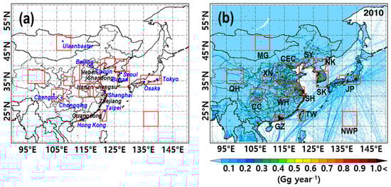
Figure 1.
(a) Fourteen analysis regions and mega-cities in this study and (b) spatial distributions of NOx emissions (0.1° × 0.1°) from the Copernicus Atmosphere Monitoring Service (CAMS) emission inventory (unit: Gg year−1).
The high NOx emissions fluxes exceeding ~1 Gg year−1 at each grid were found over the several mega-cities of China, South Korea, and Japan, whereas the remotely clean regions such as Mongolia, the western part of China, some parts of Russia, and the Northwest Pacific ocean have small emission fluxes. Thus, two groups were classified according to the strength of the NOx emission fluxes. For relatively high NOx emission fluxes, eleven regions (i.e., polluted regions) were as follow: (i) Central East China (CEC), (ii) Shanghai (SH), (iii) Wuhan (WH), (iv) Xian (XN), (v) Chongqing and Chengdu (CC), (vi) Guangzhou (GZ), (vii) Shenyang (SY), (viii) Taiwan (TW), (ix) North Korea (NK), (x) South Korea (SK), and (xi) Japan (JP). These areas are highly populated in East Asia. In contrast, three regions were selected for a remotely clean atmosphere. There are as follows: (i) Mongolia (MG), (ii) Qinghai (QH), and (iii) Northwestern Pacific Ocean (NWP).
3. Results and Discussions
Figure 2a–d represents the spatial distributions of the averaged tropospheric NO2 columns (hereafter, denoted as Ω) during the periods of ten years for 2006–2015 and two years for 2006 (actually, refer to 2006–2007), 2010 (2010–2011), and 2014 (2014–2015), respectively. As shown in Figure 1b and Figure 2, the spatial distributions of the 10-year and 2-year averaged Ω were generally consistent with those of NOx emissions, indicating that the OMI sensor well captured the emission hot-spots in the regions of CEC, SH, GZ, WH, XN, CC, SY, SK, and JP. In the analysis, the tropospheric NO2 columns were increased by 19% from 2006 to 2010, whereas those were decreased by 6% from 2010 to 2014 over the entire domain. In other words, the levels of the NO2 columns in 2014 returned to approximately those in 2006, particularly over central China. The study further focused on the features of year-to-year, monthly, and weekly variations of Ω in the 14 regions.
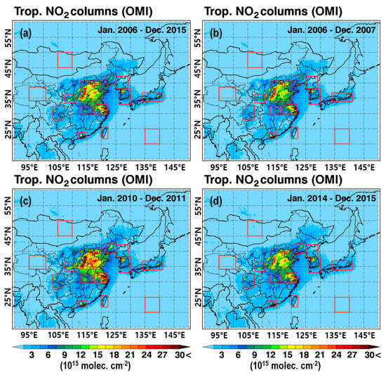
Figure 2.
(a) Tropospheric NO2 columns 10-year averaged (a) from 2006 to 2015, and 2-year averages for (b) 2006, (c) 2010, and (d) 2014 (unit: 1015 molec. cm−2).
3.1. Trend and Monthly Variations of Tropospheric NO2 Columns
The variations of monthly averaged Ω denoted as black open circles in the left panel of Figure 3 and Figure S1 (in the supplementary materials), showed cyclical patterns over most of the regions. Several investigators reported such clear cycles of Ω in East Asia e.g., references [28,30,49,50]. The variations in Ω are related to several issues of the atmospheric chemical mechanism (e.g., NOx chemical losses), the (anthropogenic, biogenic, and natural) NOx emissions, and meteorological factors [14,15,31].
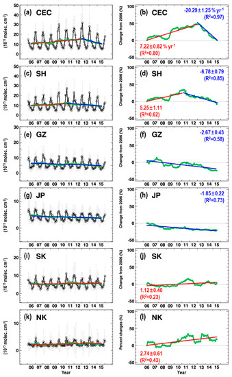
Figure 3.
Left panel represents the monthly variations of tropospheric NO2 columns (1015 molecules cm−2) over (a) Central East China (CEC), (c) Shanghai (SH), (e) Guangzhou (GZ), (g) Japan (JP), (i) South Korea (SK), and (k) North Korea (NK). Gray error bars in the left panel are 1-σ standard deviations. Here, green circle lines represent the 12-month moving averages. Red and blue lines represent the increase and/or decrease trends, respectively, which are calculated from the 12-month moving averages. The right panel represents relative changes (%) in NO2 columns from 2006 over (b) Central East China (CEC), (d) Shanghai (SH), (f) Guangzhou (GZ), (h) Japan (JP), (j) South Korea (SK), and (l) North Korea (NK). Others are as in the left panel except for the y-axis.
For example, as shown in the left panel of Figure 3, Ω increase during the cold seasons owing to fuel consumption for heating [51]. Also, low Ω are caused by the active photochemical removals of atmospheric NOx via the reactions with OH radicals during the warm seasons [14,31]. The irregular cycle of Ω partly found over NK is possibly related to insufficient electricity supplies and in-active energy consumption due to the economic instability in North Korea [52]. Moreover, because of some uncertainty of NO2 retrieval [38], the low absolute signal of NO2 columns in North Korea can contribute such an irregular pattern, which was confirmed over NWP.
The 12-month moving averages calculated from the monthly mean Ω were also plotted, as thick green lines in Figure 3. The moving average approach minimizes the random fluctuations (e.g., for NK in Figure S1) and removes a monthly effect in a long-term dataset. From the analysis of the 12-month moving averages, the variations of the NO2 columns were classified into the following four trends: (i) upward and downward trend; (ii) downward trend; (iii) stagnant trend; (iv) upward trend. Table 1 (and Table S1) summarized the (percent) increasing or decreasing rates over the fourteen regions. Over CEC, SH, XN, WH, SY, and CC, the ‘upward and downward’ trends were observed. The gradual increases in Ω were captured until the year around 2011 or 2012 apart from the periods of the global economic recession, 2008 Olympic Games in Beijing, and World Expo 2010 in Shanghai [53,54,55]. After the turning point, the moving averages declined sharply. For example, over CEC, the tropospheric NO2 columns increased at the rate of 0.75 ± 0.08 × 10¹⁵ molecules cm−2 year−1 (or 7.22 ± 0.82% year−1; data mean ± confident level of 95%) from June 2006 to November 2012 and then decreased at the rate of (−2.10 ± 0.13) × 1015 molecules cm−2 year−1 (or −20.29 ± 1.25% year−1) from November 2012 to June 2015. For SH, the NO2 column showed growth of (0.50 ± 0.11) × 1015 molecules cm−2 year−1 (or 5.25 ± 1.11% year−1) from June 2006 to January 2011 and decline of (−0.64 ± 0.07) × 1015 molecules cm−2 year−1 (or −6.78 ± 0.79% year−1) from January 2011 to June 2015. Such recent decreases in Ω over these regions were also reported previously in other studies [28,35]. For the second group, the ‘downward’ trends were observed over GZ, JP, and TW throughout the entire periods. Here, the peak in Ω would be before 2006 at least. The NO2 columns decreased at the rates of −1.6–−2.7% year−1, which were slower than those shown in other studies [26,56]. Itahashi et al. and Cui et al. reported the declines of −4.6% year−1 (from 2005 to 2008) and −3.3 ± 0.3% year− (from 2005 to 2013) over Japan and the Pearl River Delta, respectively. Also, Lee et al. [57] reported the rate of (−0.09 ± 0.01) × 1015 molecules cm−2 year−1 from 2005 to 2015 in Taiwan, which is a sharper decline than this result of (−0.05 ± 0.01) × 1015 molecules cm−2 year−1 over TW. The slight differences may be due to a different time window and base year for the different spatial regions.

Table 1.
Increasing or decreasing rates based on the 12-month moving averages.
Thirdly, the tropospheric NO2 columns increased at the slowest rate of 1.12 ± 0.40% year−1 ((0.06 ± 0.02) × 1015 molecules cm−2 year−1) over SK. Despite the slow growth, the trend was defined as stagnation because the NO2 columns seemed to be repeatedly downward-stagnant-upward moving, leading to a low correlation coefficient (R2 = 0.23). Itahashi et al. also reported such constant variation in Ω calculated and observed from the chemistry transport model and OMI sensor over SK [56]. For the last group, the ‘upward’ trends were shown over NK, MG, QH, and NWP, where Ω were relatively low. The atmospheric levels of Ω over MG, QH, and NWP (e.g., less than 1.0 × 10¹⁵ molecules cm−2) can be considered, as background levels in East Asia. The growths of Ω were (0.06 ± 0.01) × 1015 molecules cm−2 year−1 (2.74 ± 0.61% year−1) over NK, (0.02 ± 0.002) × 1015 molecules cm−2 year−1 (3.99 ± 0.30% year−1) over MG, (0.02 ± 0.002) × 1015 molecules cm−2 year−1 (4.07 ± 0.17% year−1) over QH, and (0.01 ± 0.001) × 1015 molecules cm−2 year−1 (1.81 ± 0.51% year−1) over NWP. As shown in Figure 3 and Figure S1, the 12-month moving averages were close to the linear regression line, particularly for MG and QH (R2 = 0.87 and 0.96, respectively).
In this study, the interregional correlation analysis was conducted using the monthly averaged NO2 columns. Figure 4 represents a matrix of correlation coefficients between two regions during the decade. The similarity in parameters such as NOx emissions (e.g., fraction by emission sectors), transports from neighboring areas, and photochemical regime by season determines the strength of a linear relationship between two regions. In this study, their correlation coefficients (R) between the polluted regions ranged from 0.94 to 0.71, indicating a strong positive linear relationship. For example, the largest one was between WH and XN. However, there were some moderate (positive linear) relationships found from interregional CC-JP, CC-TW, CC-GZ, and JP-WH, where coefficients ranged from 0.59 to 0.68 in the specified order. The irregular cycle of monthly Ω over CC during 2006–2010 (shown in Figure S1) can lead to these types of low correlations. Also, the trends of NO2 columns over JP, TW, and GZ, which were downward trends and were somewhat different from those over CC, have an impact on the correlation. Thus, as shown in Figure 4, the correlation coefficients between CC and other regions were slightly smaller than the others.
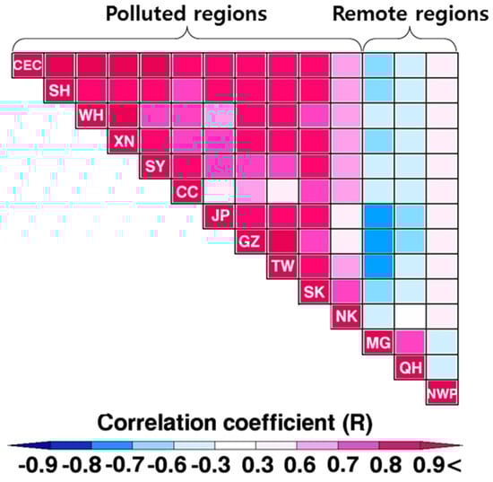
Figure 4.
Matrix view of the interregional correlations for monthly Ω between fourteen regions. Colors represent the correlation coefficients (R). Correlation rages between −1 and 1. Correlation close to 1 (or −1) indicates a more positive (or negative) relationship between the Ω over two regions. Correlation of 0 means no linear relationship. Coefficients from 0 to 0.3 (or from 0 to −0.3) indicate a week linear relationship. Coefficients from 0.3 to 0.7 (or from −0.3 to −0.7) indicate a moderate linear relationship. Coefficients from 0.7 to 1.0 (or from −0.7 to −1.0) indicate a strong linear relationship.
There are other positive linear relationships of moderate strength between NK and other polluted regions (except for SK), which ranged from 0.56 to 0.69. As discussed, insufficient electricity and inactive energy consumption are possibly related to the low correlation coefficient in North Korea, which were indirectly confirmed by the night-light images from satellite observation [52,58]. The analysis also showed lower correlations from NWP with each polluted region because NOx over the ocean is irregularly emitted from marine diesel engines and supplied by occasional long-range transports from inland [59,60].
On the other hand, there were moderate negative linear relationships (bluish color in Figure 4) for MG and QH, indicating that the monthly variations of Ω are absolutely the opposite of those over the polluted regions. The fact was found in Figure 5, showing the monthly variations of the tropospheric NO2 columns normalized to the 10-year average. Thus, Ω over MG and QH were high during the warm seasons and were low during the cold seasons in Figure 5, unlike those over the polluted regions. As intensively discussed in other studies [8,9,14,15,31], the low levels of atmospheric NO2 during the warm seasons are caused by the active NOx destruction through the reaction of NO2+OH+M→HNO3 in the urban polluted regions. In contrast, the biogenic soil NOx emissions can lead to the high levels of Ω over the rural areas (e.g., MG and QH) because microbiological activity in soil is active during the warm seasons [61,62,63,64]. Recently, Han et al. reported from their modeling study that atmospheric NO2 decomposed thermally from Peroxyacetyl Nitrates (PANs) is also a crucial contributor to the high NO2 (by up to 51%) during the warm seasons in the remote continental regions of Mongolia [31].
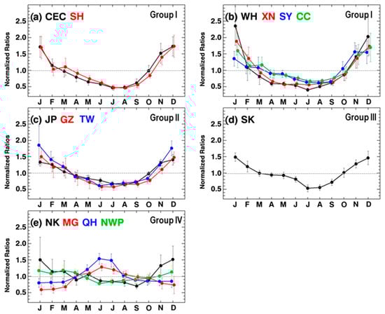
Figure 5.
Monthly variations of Ω normalized to 10-year average for each (a) CEC and SH, (b) WH, XN, SY, and CC, (c) JP, GZ, and TW, (d) SK, and (e) NK, MG, QH, and NWP. Vertical bars represent 1-σ standard deviation.
3.2. Year-to-Year Variations of Tropospheric NO2 Columns with Bottom-Up NOx Emissions
To figure out an increase or decrease in the recent Ω and to compare with the bottom-up NOx emissions, annual Ω were calculated using the monthly data. Annual averages can be a useful indicator to infer the long-term trends and validate the magnitudes of bottom-up NOx emission fluxes [27,65,66,67]. Figure S2 shows year-to-year variations of relative changes in Ω from 2006, which are similar to trends of moving averages in the right panel of Figure 3 (also, refer to annual variations of Ω in Figure S3). The negative relative changes in 2015 were observed over GZ (−24.45%), JP (−20.72%), SH (−8.63%), and TW (−8.13%). As reported in other studies [34,68,69], the policy and technical efforts on local emission control gave rise to such a decrease in Ω over these areas. Also, SH in Group I shown in Table 1 was the only region which shifted from positive to negative relative differences. In contrast, there were positive relative changes in 2015, particularly over MG, QH, NWP, and NK, which ranged from 18.20% to 46.96%. Some other regions in China showed an increase in Ω within 10%, indicating that NOx emissions for 2015 roughly returned to the magnitudes for 2006 after reaching their peaks between 2011 and 2013.
The study also analyzed the spatial distributions of NO2 columns for the years of 2006, 2011, and 2015. The year of 2011 was selected as a peak year despite some differences between regions. Figure 6 showed the spatial distribution of differences in Ω over East Asia among three reference years. Here, dark blue and dark red indicates an increase and decrease in NO2 columns, respectively. As can also be expected from Figure S2, the Ω over East Asia increased from 2006 to 2011 and then decreased from 2011 to 2015. Eventually, the levels of Ω in 2015 reached approximately levels in 2006. It is an ‘upward and downward’ trend for the entire domain. In addition, an increase or decrease in Ω can vary depending on the size of the analysis areas. For example, unlike the CEC region, the Ω in Beijing continued to decrease. In other words, unlike CEC belonging to Group I, Beijing in the urban scale analysis is rather close to the Group II defined in Table 1. As similar to those in GZ, TW, and JP in Figure S2, Figure 6 showed clear drops in NO2 columns in the cities of Hong Kong, Taipei, Tokyo, and Osaka. The reductions of Ω in the urban scales are in line with those of previous studies [33,34].
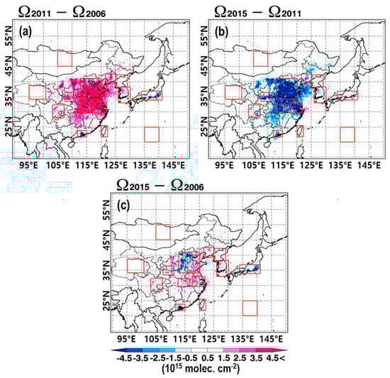
Figure 6.
Spatial distributions of NO2 column differences (a) between 2011 and 2006, (b) between 2015 and 2011, and (c) 2015 and 2006.
One more interesting finding was a distinct contrast between Hebei and Shandong provinces, as shown in CEC of Figure 6c. The positive sign around Shandong province canceled out the negative sign around Hebei province and Beijing. Such spatially different sign of ΔΩ = (Ω2015 – Ω2006) in Hebei and Shandong can be associated with the disparities implementing new emission regulations for power plants and more stringent emissions standards for vehicles in China [27,68]. The new emissions regulations planned in 2012 required that thermal power plants be upgraded or equipped with low NOx combustion technologies and flue gas denitrification (e.g., selective (non-)selective catalytic reduction). The facilities affected by this were particularly concentrated in the BTH (Beijing, Tianjin, and Hebei), Yangtze River Delta (Shanghai, Jiangsu, and Zhejiang), and Pearl River Delta (Guangdong) [27].
Despite a nonlinear relationship between NOx and NO2 in the atmosphere, this study compared the year-to-year variations of NOx emission of CAMS and CAPSS inventories with those of Ω because the satellite observed NO2 column is as a proxy for surface NOx emissions. Figure 7 and Figure S4 showed the year-to-year variations of NOx emissions and NO2 columns normalized to those in 2006 during a decade. The comparison between the two variables exhibited a good correlation coefficient (R > 0.7) in several regions of CC, SY, JP, TW, QH, and MG, indicating that the year-to-year variations of the bottom-up NOx emission from the CAMS were similar to those of Ω. This finding is consistent with those from previous studies for (western) China, Japan, and Taiwan [26,27,56,57]. However, the results over most of the other regions (e.g., CEC, SH, GZ, WH, and XN) showed lower correlation coefficients regardless of the degree of pollution. It is likely that considering the emissions data without considering the recent reduction since ~2011 in China causes these low correlations. The analysis showed that the largest sector of the power generation in CEC and SH decreased by 10% and 16%, respectively, but increases in the industrial process sector offset such decreases. As shown in Figure 7, the bottom-up NOx emissions have declined in CEC and SH regions since 2011, but only marginally.
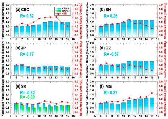
Figure 7.
Year-to-year variations of NOx emissions (blue and green bars for CAMS and CAPSS, respectively) and NO2 columns (red circles) normalized to those in 2006 for (a) CEC, (b) SH, (c) JP, (d) GZ, (e) SK, and (f) MG.
Interestingly, NO2 columns showed an inverse correlation with NOx emissions in the GZ, NK, and SK regions. In North Korea, the use of biofuel increased due to the sharp declines in coal supply since 2010 [70]. However, biological fuels were not possibly reflected in the NOx emission inventory, which led to the inverse correlation between two variables. Besides, biofuels are known to produce more air pollutants than coal and petroleum, generating the same amount of heat [70].
Overall, unlike expectations, the NOx emissions of CMAS and CAPSS inventories do not seem to adequately reflect the annual changes in Ω over many analysis regions in China, South Korea, and North Korea. Also, there is still room for improvement in the trends of NOx emission inventories.
3.3. Weekly Variations of Tropospheric NO2 Columns
The weekend effect means that the use of fossil fuels is reduced due to weak industrial and human activities during the weekend, thereby leading to low levels of air pollutants on the weekend. Beirle et al. first discussed the weekend effect of Ω in some cities of the US, Europe, and Japan using the satellite data from the GOME sensor for 1996–2001 [23]. They showed that Ω on Sunday is 25–50% small, compared with those on weekdays in these countries. This study also investigated the weekly cycles of Ω over the 14 regions in East Asia. Based on the analysis, it can provide valuable information on the weekly temporal allocation of NOx emission for the input of 3D-CTM in East Asia.
Figure 8 represents the weekly cycles of Ω normalized to the averaged Ω during a decade from 2006 to 2015 by region grouped to a similar level of variation. As shown in Figure 8a,b, the data points were distributed close to 1, indicating that there are no weekly changes in Ω in CC, QH, NWP, CEC, MG, and SY. Similarly, in WH, SH, GZ, and XN (in Figure 8c,d), Ω seem to be slightly lower on the weekend, but the normalized ratios are in the range between 0.9 and 1.1, without significant differences from the weekday. Again, from the analysis, it revealed that there is no weekly effect for several regions in China. According to the study of Beirle et al. [23], the absence of the weekend effect in China pointed out that energy production and industrial activities operating throughout the week contributes significantly to the Chinese NOx emissions. To confirm this fact, Table 2 showed each contribution of NOx emissions by sector. The analysis of the CAMS emissions showed that 72–86% of the total anthropogenic NOx is emitted mainly from power generations and industrial processes in the selected regions in China.
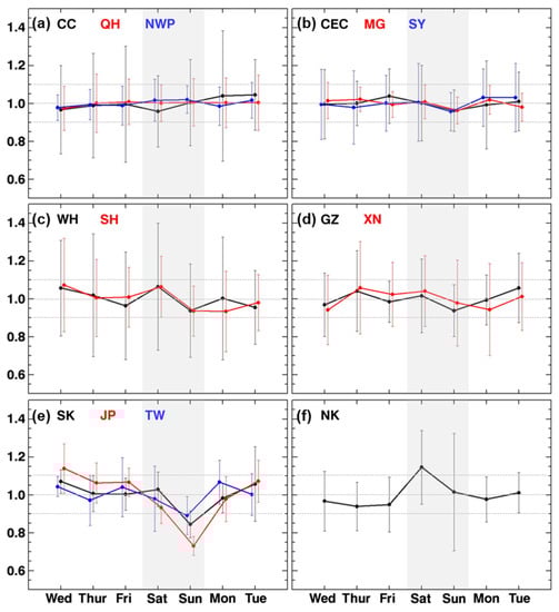
Figure 8.
Weekly cycles of Ω normalized to 10-year averaged Ω for (a) CC, QH, and NWP, (b) CEC, MG, and SY, (c) WH and SH, (d) GZ and XN, (e) SK, JP, and TW, and (f) NK. Vertical bars represent 1-σ standard deviation. Gray shaded areas represent the weekend.
Table 2.
NOx emission contribution by sector from the CAMS inventory for 2006–2015 (%).
On the other hand, Figure 8e displayed the clear weekly cycles in SK, JP, and TW, showing low and high Ω on the weekend and the workdays, respectively. The result was also consistent with previous studies [23,71]. Therefore, as expected from the clear weekly cycle, the NOx emissions in SK, JP, and TW can be affected significantly by the transportation sector. As shown in Table 2, its contribution (i.e., 20–48%) in SK, JP, and TW was much higher than those in several polluted regions of China.
In the NK regions, it is interesting that the level of Ω was rather high on Saturday (see Figure 8f). Weekly analysis for each year (from 2006 to 2015) also showed a consistent result. As an alternative of deficient coal, the increased use of biofuels for cooking and heating may be partly attributed to the unexpected weekly variation in North Korea, along with the lifestyle of North Koreans [63]. However, it was difficult to draw a firm conclusion due to the lack of reliable information and limited studies available for North Korea. Further investigations are required.
The relative differences between two NO2 columns on the weekend (ΩWKND) and the weekday (ΩWKDY) were calculated using the Equation (1) to quantify the weekend effect in East Asia.
Figure 9 showed the spatial distributions of the relative differences over East Asia. Here, the bluish color represents the weekend effect (or lower Ω on the weekend). The reddish color over several regions of China can be attributed to energy production and industrial activities throughout the week, as previously discussed. However, the reddish color in NWP would be differently made by NOx sources from irregular ship emissions (refer to Table 2). Also, time lag during transport of NOx plume from inland via a westerly wind (~1 day, particularly, in winter) can hamper the relative difference. As shown in Figure 9, the dark blue was distributed mainly in SK and JP. In the analysis, NO2 columns were 5.1%, 5.6%, and 15.1% lower on the weekend in SK, TW, and JP, respectively. These relative differences were quite smaller than those (approximately −25–−50%) in the cities of the US and Europe [23,72,73] because of the larger size of the target areas in this study. In the urban scale analysis, the (negative) relative differences in the megacities of Taipei (−18.1%), Seoul (−19.9%), Busan (−27.3%), Osaka (−32.1%), and Tokyo (−33.4%) were closer to those in the cities of the US and Europe. Considering data only on Sunday for the weekend effect, the relative differences in the magnitude would be much higher. For other cities, the relative differences were −2.8% in Shanghai, −3.7% in Hong Kong, −12.0% in Chengdu, and −14.2% in Chongqing, which is a slight weekend effect. However, over Beijing (1.1%) and Tianjin (0.1%), positive relative differences were found.
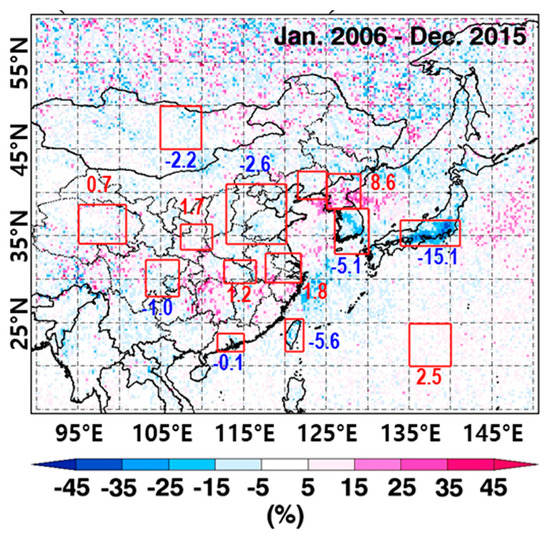
Figure 9.
Spatial map of the relative differences between the NO2 columns on the weekend (ΩWKND) and weekday (ΩWKDY) during the period 2006–2015. The blue and red numbers given in the figure represent the relative differences for the analysis regions.
4. Summaries and Conclusions
In the study, temporal analysis of tropospheric NO2 columns was carried out over fourteen areas based on a regional scale in East Asia using the OMI-observed data during the period from 2006 to 2015. The monthly variations of the NO2 columns governed by the combined issues of NOx emissions, chemical mechanism, and meteorological fields showed a cyclical pattern over most of the analysis regions. The 12-month moving averages from these monthly Ω were calculated to analyze the trends of Ω over East Asia. The 12-month moving averages were close to the linear trend lines, with good correlation coefficients over most of the analysis regions. The trends were classified into four groups: (i) upward and downward; (ii) downward; (iii) stagnant; (iv) upward trends. First, the ‘upward and downward’ trend was from CEC, SH, XN, WH, SY, and CC. After the maximum of Ω around the year of 2011–2012, the moving averages declined sharply. For example, over CEC, the Ω increased at the rate of 0.75(±0.08) × 1015 molecules cm−2 year−1 from June 2006 to November 2012 and then decreased at the rate of −2.10(±0.13) × 1015 molecules cm−2 year−1 from November 2012 to June 2015. Second, the ‘downward’ trend was observed over GZ, JP, and TW. The Ω decreased at the rates of (−0.05(±0.01)–−0.16(±0.01)) × 1015 molecules cm−2 year−1 over these regions. Third, the ‘stagnant’ trend was shown over SK. Fourth, the ‘upward’ trend was shown over NK, MG, QH, and NWP. The growth of Ω was (0.01(±0.001)–0.06(±0.01)) × 1015 molecules cm−2 year−1. Overall, the levels of tropospheric NO2 columns in 2015 returned to the magnitudes in 2006 over most of the polluted regions in China. From the annual data analysis, the relative change of NO2 columns in 2015 compared to those in 2006 were approximately 10% for most of the regions in China.
The monthly averaged Ω was utilized to investigate the interregional correlation. The analysis can provide useful information on similarities in NOx emission by sector or atmospheric photochemistry by season between two analysis regions. The investigation showed strong positive linear relationships (0.94 >R > 0.71) between most of the polluted areas, including CEC and SH, and moderate positive linear one (0.69 > R > 0.56) found between CC and other regions of JP, TW, and GZ. On the other hand, the different variations of NO2 columns led to negative relationships in MG and QH.
The variations of Ω were compared with those of bottom-up NOx emissions from the CAMS and CAPSS inventories because NO2 column is a proxy for NOx emissions. The NO2 columns were strongly correlated to NOx emissions over CC, SY, JP, TW, QH, and MG (R > 0.7), whereas the comparison showed low correlation coefficients over most other regions. The low correlations were caused by emission data without considering the recent reduction in NOx emissions after ~2011 in China. From the comparison study, the NOx emissions from the CAMS and CAPSS inventories do not appear to follow the annual changes in Ω over CEC, SH, GZ, SK, WH, XN, and NK.
In the investigation on the weekly cycle of Ω, no significant weekly effects were observed in most regions of China. This indicates that industrial activities throughout the week contribute significantly to the Chinese NOx emissions. In the budget analysis of the CAMS NOx inventory, the contribution was 72–86% from power generation and industrial processes over the Chinese regions. On the other hand, the weekly effect was clearly shown in SK, JP, and TW, which is in line with other previous studies. Also, the result indicates that NOx emissions over these regions were significantly affected by the transportation sector. The contributions were 48%, 20%, and 40% over SK, JP, and TW, respectively. Moreover, a characteristic feature was found over NK showing high levels of NO2 columns on Saturday.
Overall, from the analysis of the OMI-retrieved tropospheric NO2 columns, the results of temporal variations can be useful information for validation of NOx emissions inventory (e.g., CAMS and CAPSS) to improve the accuracy of the air quality forecasting. In the future, if a geostationary satellite such as Geostationary Environment Monitoring Spectrometer (GEMS) [74] is successfully launched and operated, improved spatio-temporal resolution data will be provided to enable more sophisticated analysis of NO2 columns over Asia.
Supplementary Materials
The following are available online at https://www.mdpi.com/2073-4433/10/11/658/s1, Figure S1: As Figure 3, except for WH, SY, XN, CC, TW, MG, QH, and NWP., Figure S2: Annual variations of NO2 column changes (%) from 2006 for each (a) CEC and SH, (b) WH, XN, SY, and CC, (c) JP, GZ, and TW, (d) SK, and (e) NK, MG, QH, and NWP. (f) as Figure S2a–e, except for the variations by groups defined in Table 1., Figure S3: Annual variations of NO2 column for (a) CEC and SH, (b) WH, XN, SY, and CC, (c) JP, GZ, and TW, (d) SK, and (e) NK, MG, QH, and NWP., Figure S4: As Figure 7, except for WH, SY, XN, CC, TW, NK, QH, and NWP., Table S1: Annual percent increasing or decreasing rates based on the 12-month moving averages.
Funding
This work was supported by National Research Foundation of Korea Grant from the Korean Government (MSIT; the Ministry of Science and ICT) (NRF-2016M1A5A1027157) (KOPRI-PN18081). This work was also supported by the National Strategic Project-Fine particle of the National Research Foundation of Korea (NRF), and the Ministry of Science and ICT (MSIT), the Ministry of Environment (ME), and the Ministry of Health and Welfare (MOHW) (NRF- 2017M3D8A1092022).
Acknowledgments
The author would like to acknowledge the use of the emission data (Copernicus Atmospheric Monitoring Service; Clean Air Policy Support System) from the ECCAD website (https://eccad.aeris-data.fr/) in EU and National Air Pollutants Emissions Service (http://airemiss.nier.go.kr/) in Korea. Also, the author is sincerely thankful for the free use of tropospheric NO2 columns from TEMIS portal (www.temis.nl).
Conflicts of Interest
The author declares no conflict of interest.
References
- European Environment Agency (EEA). Annual European Community LRTAP Convention Emissions Inventory Report 1990–2006; No 7/2008; EEA: Copenhagen, Denmark, 2008; pp. 1–79. [Google Scholar]
- US Environmental Protection Agency (US EPA). 2008 National Emissions Inventory: Review, Analysis and Highlights; EPA-454/R-13-005; US EPA: Washington, DC, USA, 2013; pp. 1–70.
- Yienger, J.I.; Levy, H., II. Empirical model of global soil-biogenic NOx emissions. J. Geophys. Res. 1995, 100, 11447–11464. [Google Scholar] [CrossRef]
- Vinken, G.C.M.; Boersma, K.F.; Maasakkers, J.D.; Adon, M.; Martin, R.V. Worldwide biogenic soil NOx emissions inferred from OMI NO2 observations. Atmos. Chem. Phys. 2014, 14, 10363–10381. [Google Scholar] [CrossRef]
- Martin, R.V.; Chance, K.; Jacob, D.J.; Kurosu, T.P.; Spurr, R.J.D.; Bucsela, E.; Gleason, J.F.; Palmer, P.I.; Bey, I.; Fiore, A.M.; et al. An improved retrieval of tropospheric nitrogen dioxide from GOME. J. Geophys. Res. 2002, 107, ACH-9. [Google Scholar] [CrossRef]
- Jaeglé, L.; Steinberger, L.; Martin, R.V.; Chance, K. Global partitioning of NOx sources using satellite observations: Relative roles of fossil fuel combustion, biomass burning and soil emissions. Faraday Discuss. 2005, 130, 407–423. [Google Scholar] [CrossRef] [PubMed]
- van Noije, T.P.C.; Eskes, H.J.; Dentener, F.J.; Stevenson, D.S.; Ellingsen, K.; Schultz, M.G.; Wild, O.; Amann, M.; Atherton, C.S.; Bergmann, D.J.; et al. Multi-model ensemble simulations of tropospheric NO2 compared with GOME retrievals for the year 2000. Atmos. Chem. Phys. 2006, 6, 2943–2979. [Google Scholar] [CrossRef]
- Han, K.M.; Song, C.H.; Ahn, H.J.; Park, R.S.; Woo, J.H.; Lee, C.K.; Richter, A.; Burrows, J.P.; Kim, J.Y.; Hong, J.H. Investigation of NOx emissions and NOx-related chemistry in East Asia using CMAQ-predicted and GOME-derived NO2 columns. Atmos. Chem. Phys. 2009, 9, 1017–1036. [Google Scholar] [CrossRef]
- Han, K.M.; Lee, S.; Chang, L.S.; Song, C.H. A comparison study between CMAQ-simulated and OMI-retrieved NO2 columns over East Asia for evaluation of NOx emission fluxes of INTEX-B, CAPSS, and REAS inventories. Atmos. Chem. Phys. 2015, 15, 1913–1938. [Google Scholar] [CrossRef][Green Version]
- McLinden, C.A.; Fioletov, V.; Krotkov, N.A.; Li, C.; Boersma, K.F.; Adams, C. A decade of change in NO2 and SO2 over the Canadian oil sands as seen from space. Environ. Sci. Technol. 2015, 50, 331–337. [Google Scholar] [CrossRef]
- Majid, A.; val Martin, M.; Lamsal, L.N.; Duncan, B.N. A decade of changes in nitrogen oxides over regions of oil and natural gas activity in the United States. Elem. Sci. Anthr. 2017, 5, 76. [Google Scholar] [CrossRef]
- Martin, R.V.; Sioris, C.E.; Chance, K.; Ryerson, T.B.; Bertram, T.H.; Wooldridge, P.J.; Cohen, R.C.; Neuman, J.A.; Swanson, A.; Flocke, F.M. Evaluation of space-based constraints on global nitrogen oxide emissions with regional aircraft measurements over and downwind of eastern North America. J. Geophys. Res. 2006, 111, D15308. [Google Scholar] [CrossRef]
- Zhao, C.; Wang, Y. Assimilated inversion of NOx emissions over east Asia using OMI NO2 column measurements. Geophys. Res. Lett. 2009, 36, L06805. [Google Scholar] [CrossRef]
- Lamsal, L.N.; Martin, R.V.; van Donkelaar, A.; Celarier, E.A.; Bucsela, E.J.; Boersma, K.F.; Dirksen, R.; Luo, C.; Wang, Y. Indirect validation of tropospheric nitrogen dioxide retrieved from the OMI satellite instrument: Insight into the seasonal variation of nitrogen oxides at northern midlatitudes. J. Geophys. Res. 2010, 115, D05302. [Google Scholar] [CrossRef]
- Lin, J.T.; McElroy, M.B.; Boersma, K.F. Constraint of anthropogenic NOx emissions in China from different sectors: A new methodology using multiple satellite retrievals. Atmos. Chem. Phys. 2010, 10, 63–78. [Google Scholar] [CrossRef]
- Mijling, B.; van der A, R.J. Using daily satellite observations to estimate emissions of short-lived air pollutants on a mesoscopic scale. J. Geophys. Res. 2012, 117. [Google Scholar] [CrossRef]
- Qu, Z.; Henze, D.K.; Capps, S.L.; Wang, Y.; Xu, X.; Wang, J.; Keller, M. Monthly top-down NOx emissions for China (2005–2012): A hybrid inversion method and trend analysis. J. Geophys. Res. Atmos. 2017, 122, 4600–4625. [Google Scholar] [CrossRef]
- Miyazaki, K.; Eskes, H.; Sudo, K.; Boersma, K.F.; Bowman, K.; Kanaya, Y. Decadal changes in global surface NOx emissions from multi-constituent satellite data assimilation. Atmos. Chem. Phys. 2017, 17, 807–837. [Google Scholar] [CrossRef]
- Lee, H.J.; Kim, S.W.; Brioude, J.; Cooper, O.R.; Frost, G.J.; Kim, C.H.; Park, R.J.; Trainer, M.; Woo, J.H. Transport of NOx in East Asia identified by satellite and in situ measurements and Lagrangian particle dispersion model simulations. J. Geophys. Res. Atmos. 2014, 119, 2574–2596. [Google Scholar] [CrossRef]
- Schere, K.; Flemming, J.; Vautard, R.; Chemel, C.; Colette, A.; Hogrefe, C.; Bessagnet, B.; Meleux, F.; Mathur, R.; Roselle, S.; et al. Trace gas/aerosol boundary concentrations and their impacts on continental-scale AQMEII modeling domains. Atmos. Environ. 2012, 53, 38–50. [Google Scholar] [CrossRef][Green Version]
- Giordano, L.; Brunner, D.; Flemming, J.; Hogrefe, C.; Im, U.; Bianconi, R.; Badia, A.; Balzarini, A.; Barò, R.; Chemel, C.; et al. Assessment of the MACC reanalysis and its influence as chemical boundary conditions for regional air quality modeling in AQMEII-2. Atmos. Environ. 2015, 115, 371–388. [Google Scholar] [CrossRef]
- GlobEmission. Available online: http://www.globemission.eu/data.php (accessed on 11 September 2019).
- Beirle, S.; Platt, U.; Wenig, M.; Wagner, T. Weekly cycle of NO2 by GOME measurements: A signature of anthropogenic sources. Atmos. Chem. Phys. 2003, 3, 2225–2232. [Google Scholar] [CrossRef]
- van der A, R.J.; Eskes, H.J.; Boersma, K.F.; van Noije, T.P.C.; van Roozendael, M.; de Smedt, I.; Peters, D.H.M.U.; Meijer, E.W. Trends, seasonal variability and dominant NOx source derived from a ten year record of NO2 measured from space. J. Geophys. Res. Atmos. 2008, 113, D04302. [Google Scholar] [CrossRef]
- Valin, L.C.; Russell, A.R.; Cohen, R.C. Chemical feedback effects on the spatial patterns of the NOx weekend effect: A sensitivity analysis. Atmos. Chem. Phys. 2014, 14, 1–9. [Google Scholar] [CrossRef]
- Cui, Y.; Lin, J.; Song, C.; Liu, M.; Yan, Y.; Xu, Y.; Huang, B. Rapid growth in nitrogen dioxide pollution over Western China, 2005–2013. Atmos. Chem. Phys. 2016, 16, 6207–6221. [Google Scholar] [CrossRef]
- Liu, F.; Zhang, Q.; van der A, R.J.; Zheng, B.; Tong, D.; Yan, L.; Zheng, Y.; He, K. Recent reduction in NOx emissions over China; synthesis of satellite observations and emission inventories. Environ. Res. Lett. 2016, 11, 114002. [Google Scholar] [CrossRef]
- Zhang, L.; Lee, C.S.; Zhang, R.; Chen, L. Spatial and temporal evaluation of long term trend (2005–2014) of OMI retrieved NO2 and SO2 concentrations in Henan Province, China. Atmos. Environ. 2017, 154, 151–166. [Google Scholar] [CrossRef]
- Jiang, Z.; McDonald, B.C.; Worden, H.; Worden, J.R.; Miyazaki, K.; Qu, Z.; Henze, D.K.; Jones, D.B.A.; Arellano, A.F.; Fischer, E.V.; et al. Unexpected slowdown of US pollutant emission reduction in the past decade. Proc. Natl. Acad. Sci. USA 2018, 115, 5099–5104. [Google Scholar] [CrossRef]
- Zheng, C.; Zhao, C.; Li, Y.; Wu, X.; Zhang, K.; Gao, J.; Qiao, Q.; Ren, Y.; Zhang, X.; Chai, F. Spatial and temporal distribution of NO2 and SO2 in Inner Mongolia urban agglomeration obtained from satellite remote sensing and ground observations. Atmos. Environ. 2018, 188, 50–59. [Google Scholar] [CrossRef]
- Han, K.M.; Lee, S.; Yoon, Y.J.; Lee, B.Y.; Song, C.H. A model investigation into the atmospheric NOy chemistry in remote continental Asia. Atmos. Environ. 2019, 214, 116817. [Google Scholar] [CrossRef]
- Cleveland, W.S.; Graedel, T.E.; Kleiner, B.; Warner, J.L. Sunday and workday variations in photochemical air pollutions in New Jersey and New York. Science 1974, 186, 1037–1038. [Google Scholar] [CrossRef]
- de Foy, B.; Lu, Z.; Streets, D.G. Satellite NO2 retrievals suggest China has exceeded its NOx reduction goals from the twelfth Five-Year Plan. Sci. Rep. 2016, 6, 35912. [Google Scholar] [CrossRef]
- Duncan, B.N.; Lamsal, L.N.; Thompson, A.M.; Yoshida, Y.; Lu, Z.; Streets, D.G.; Hurwitz, M.M.; Pickering, K.E. A space-based, high-resolution view of notable changes in urban NOx pollution around the world (2005–2014). J. Geophys. Res. Atmos. 2016, 121, 976–996. [Google Scholar] [CrossRef]
- Krotkov, N.A.; McLinden, C.A.; Li, C.; Lamsal, L.N.; Celarier, E.A.; Marchenko, S.V.; Swartz, W.H.; Bucsela, E.J.; Joiner, J.; Duncan, B.N.; et al. Aura OMI observations of regional SO2 and NO2 pollution changes from 2005 to 2015. Atmos. Chem. Phys. 2016, 16, 4605–4629. [Google Scholar] [CrossRef]
- Levelt, P.F.; van den Oord, G.H.J.; Dobber, M.R.; Mälkki, A.; Visser, H.; de Vries, J.; Stammes, P.; Lundell, J.O.V.; Saari, H. The ozone monitoring instrument. IEEE Trans. Geosci. Remote Sens. 2006, 44, 1093–1100. [Google Scholar] [CrossRef]
- Boersma, K.F.; Braak, R.; van der A, R.J. Dutch OMI NO2 (DOMINO) Data Product v2.0 HE5 Data File User Manual; Royal Netherlands Meteorological Institute (KNMI): De Bilt, The Netherlands, 2011; pp. 1–21. [Google Scholar]
- Boersma, K.F.; Eskes, H.J.; Dirksen, R.J.; van der A, R.J.; Veefkind, J.P.; Stammes, P.; Huijnen, V.; Kleipool, Q.L.; Sneep, M.; Claas, J.; et al. An improved tropospheric NO2 column retrieval algorithm for the Ozone Monitoring Instrument. Atmos. Meas. Tech. 2011, 4, 1905–1928. [Google Scholar] [CrossRef]
- Tropospheric Emission Monitoring Internet Service (TEMIS). Available online: http://www.temis.nl (accessed on 11 September 2019).
- Boersma, K.F.; Eskes, H.J.; Veefkind, J.P.; Brinksma, E.J.; van der A, R.J.; Sneep, M.; van den Oord, G.H.J.; Levelt, P.F.; Stammes, P.; Gleason, J.F.; et al. Near-real time retrieval of tropospheric NO2 from OMI. Atmos. Chem. Phys. 2007, 7, 2103–2118. [Google Scholar] [CrossRef]
- Platt, U. Differential optical absorption spectroscopy (DOAS). Chem. Anal. Ser. 1994, 127, 27–83. [Google Scholar]
- Stammes, P. Spectral radiance modelling in the UV-Visible range. In IRS 2000: Current Problems in Atmospheric Radiation; Smith, W.L., Timofeyev, Y.M., Eds.; A. Deepak Publ.: Hampton, VA, USA, 2001; pp. 385–388. [Google Scholar]
- Zhang, R.; Wang, Y.; Smeltzer, C.; Qu, H.; Koshak, W.; Boersma, K.F. Comparing OMI-based and EPA AQS in situ NO2 trends: Towards understanding surface NOx emission changes. Atmos. Meas. Tech. 2018, 11, 3955–3967. [Google Scholar] [CrossRef]
- Lin, J.-T.; Liu, M.-Y.; Xin, J.-Y.; Boersma, K.F.; Spurr, R.; Martin, R.; Zhang, Q. Influence of aerosols and surface reflectance on satellite NO2 retrieval: Seasonal and spatial characteristics and implications for NOx emission constraints. Atmos. Chem. Phys. 2015, 15, 11217–11241. [Google Scholar] [CrossRef]
- Emissions of atmospheric Compounds and Compilation of Ancillary Data (ECCAD). Available online: https://eccad.aeris-data.fr/ (accessed on 11 September 2019).
- Clean Air Policy Support System (CAPSS). Available online: http://airemiss.nier.go.kr/ (accessed on 11 September 2019).
- Zheng, B.; Tong, D.; Li, M.; Liu, F.; Hong, C.; Geng, G.; Li, H.; Li, X.; Peng, L.; Qi, J.; et al. Trends in China’s anthropogenic emissions since 2010 as the consequence of clean air actions. Atmos. Chem. Phys. 2018, 18, 14095–14111. [Google Scholar] [CrossRef]
- Granier, C.; Darras, S.; van der Gon, H.D.; Doubalova, J.; Elguindi, N.; Galle, B.; Gauss, M.; Guevara, M.; Jalkanen, J.P.; Kuenen, J.; et al. The Copernicus Atmosphere Monitoring Service global and regional emissions (April 2019 version). CAMS Rep. 2019, 1–54. [Google Scholar] [CrossRef]
- Hilboll, A.; Richter, A.; Burrows, J.P. Long-term changes of tropospheric NO2 over megacities derived from multiple satellite instruments. Atmos. Chem. Phys. 2013, 13, 4145–4169. [Google Scholar] [CrossRef]
- Kanaya, Y.; Irie, H.; Takashima, H.; Iwabuchi, H.; Akimoto, H.; Sudo, K.; Gu, M.; Chong, J.; Kim, Y.J.; Lee, H.; et al. Long-term MAX-DOAS network observations of NO2 in Russia and Asia (MADRAS) during the period 2007–2012: Instrumentation, elucidation of climatology, and comparisons with OMI satellite observations and global model simulations. Atmos. Chem. Phys. 2014, 14, 7909–7927. [Google Scholar] [CrossRef]
- Wang, C.; Wang, T.; Wang, P. The spatial-temporal variation of tropospheric NO2 over China during 2005 to 2018. Atmosphere 2019, 10, 444. [Google Scholar] [CrossRef]
- Han, K.M.; Lee, C.K.; Lee, J.; Kim, J.; Song, C.H. A comparison study between model-predicted and OMI-retrieved tropospheric NO2 columns over the Korean peninsula. Atmos. Environ. 2011, 45, 2962–2971. [Google Scholar] [CrossRef]
- Lin, J.T.; Nielsen, C.P.; Zhao, Y.; Lei, Y.; Liu, Y.; McElroy, M.B. Recent changes in particulate air pollution over China observed from space and the ground: Effectiveness of emission control. Environ. Sci. Technol. 2010, 44, 7771–7776. [Google Scholar] [CrossRef]
- Mijling, B.; van der A, R.J.; Boersma, K.F.; van Roozendael, M.; de Smedt, I.; Kelder, H.M. Reductions of NO2 detected from space during the 2008 Beijing Olympic Games. Geophy. Res. Lett. 2009, 36, L13801. [Google Scholar] [CrossRef]
- Hao, N.; Valk, P.; Loyola, D.; Cheng, Y.F.; Zimmer, W. Space-based measurements of air quality during the World Expo 2010 in Shanghai. Environ. Res. Lett. 2011, 6, 044004. [Google Scholar] [CrossRef]
- Itahashi, S.; Uno, I.; Irie, H.; Kurokawa, J.I.; Ohara, T. Regional modeling of tropospheric NO2 vertical column density over East Asia during the period 2000–2010: Comparison with multisatellite observations. Atmos. Chem. Phys. 2014, 14, 3623–3635. [Google Scholar] [CrossRef]
- Lee, C.H.; Chang, K.H.; Kim, H. Long-term (2005–2015) trend analysis of OMI retrieved NO2 columns in Taiwan. Atmos. Pollut. Res. 2019, 10, 960–970. [Google Scholar] [CrossRef]
- Miller, S.D.; Mills, S.P.; Elvidge, C.D.; Lindsey, D.T.; Lee, T.F.; Hawkins, J.D. Suomi satellite brings to light a unique frontier of nighttime environmental sensing capabilities. PNAS 2012, 109, 15706–15711. [Google Scholar] [CrossRef]
- Wenig, M.; Spichtinger, N.; Stohl, A.; Held, G.; Beirle, S.; Wagner, T.; Jähne, B.; Platt, U. Intercontinental transport of nitrogen oxide pollution plumes. Atmos. Chem. Phys. 2003, 3, 387–393. [Google Scholar] [CrossRef]
- Wan, Z.; Zhu, M.; Chen, S.; Sperling, D. Pollution: Three steps to a green shipping industry. Nature 2016, 230, 275–277. [Google Scholar] [CrossRef] [PubMed]
- Hudman, R.C.; Russell, A.R.; Valin, L.C.; Cohen, R.C. Interannual variability in soil nitric oxide emissions over the United States as viewed from space. Atmos. Chem. Phys. 2010, 10, 9943–9952. [Google Scholar] [CrossRef]
- Oikawa, P.Y.; Ge, C.; Wang, J.; Eberwein, J.R.; Liang, L.L.; Allsman, L.A.; Grantz, D.A.; Jenerette, G.D. Unusually high soil nitrogen oxide emissions influence air quality in a high-temperature agricultural region. Nat. Commun. 2015, 6, 8753. [Google Scholar] [CrossRef]
- van der A, R.J.; Peters, D.H.M.U.; Eskes, E.; Boersma, K.F.; van Roozendael, M. Detection of the trend and seasonal variation in tropospheric NO2 over China. J. Geophys. Res. 2006, 111, D12317. [Google Scholar] [CrossRef]
- Holland, E.; Dentener, F.J.; Braswell, B.H.; Sulzman, J.M. Contemporary and pre-industrial global reactive nitrogen budgets. Biogeochemistry 1999, 46, 7–43. [Google Scholar] [CrossRef]
- Martin, R.V.; Jacob, D.J.; Chance, K.; Kurosu, T.P.; Palmer, P.I.; Evans, M.J. Global inventory of nitrogen oxide emissions constrained by space-based observations of NO2 columns. J. Geophys. Res. Atmos. 2003, 108. [Google Scholar] [CrossRef]
- Richter, A.; Burrows, J.P.; Nüß, H.; Granier, C.; Niemeier, U. Increase in tropospheric nitrogen dioxide over China observed from space. Nature 2005, 437, 129–132. [Google Scholar] [CrossRef]
- Silvern, R.F.; Jacob, D.J.; Mickley, L.J.; Sulprizio, M.P.; Travis, K.R.; Marais, E.A.; Cohen, R.C.; Laughner, J.L.; Choi, S.; Joiner, J.; et al. Using satellite observations of tropospheric NO2 columns to infer long-term trends in US NOx emissions: The importance of accounting for the free tropospheric NO2 background. Atmos. Chem. Phys. 2019, 19, 8863–8878. [Google Scholar] [CrossRef]
- Zhao, B.; Wang, S.X.; Liu, H.; Xu, J.Y.; Fu, K.; Klimont, Z.; Hao, J.M.; He, K.B.; Cofala, J.; Amann, M. NOx emissions in China: Historical trends and future perspectives. Atmos. Chem. Phys. 2013, 13, 9869–9897. [Google Scholar] [CrossRef]
- Zhong, L.; Louie, P.K.K.; Zheng, J.; Wai, K.M.; Ho, J.W.K.; Yuan, Z.; Lau, A.K.H.; Yue, D.; Zhou, Y. The Pearl River Delta regional air quality monitoring network—Regional collaborative efforts on joint air quality management. Aerosol Air Qual. Res. 2013, 13, 1582–1597. [Google Scholar] [CrossRef]
- Kim, I.S.; Kim, Y.P. Characteristics of energy usage and emissions of air pollutants in North Korea. J. Korean Soc. Atmos. Environ. 2019, 35, 125–137. [Google Scholar] [CrossRef]
- Judd, L.M.; Al-Saadi, J.A.; Valin, L.C.; Pierce, R.B.; Yang, K.; Janz, S.J.; Kowalewski, M.G.; Szykman, J.J.; Tiefengraber, M.; Mueller, M. The dawn of geostationary air quality monitoring: Case studies from Seoul and Los Angeles. Front. Environ. Sci. 2018, 6, 85. [Google Scholar] [CrossRef] [PubMed]
- de Foy, B.; Lu, Z.; Streets, D.G. Impacts of control strategies, the great recession and weekday variations on NO2 columns above North American cities. Atmos. Environ. 2018, 138, 74–86. [Google Scholar] [CrossRef]
- Ialongo, I.; Herman, J.; Krotkov, N.; Lamsal, L.; Boersma, K.F.; Hovila, J.; Tamminen, J. Comparison of OMI NO2 observations and their seasonal and weekly cycles with ground-based measurements in Helsinki. Atmos. Meas. Tech. 2016, 9, 5203–5212. [Google Scholar] [CrossRef]
- Kim, J.; Jeong, U.; Ahn, M.; Kim, J.H.; Park, R.J.; Lee, H.; Song, C.H.; Choi, Y.S.; Lee, K.H.; Yoo, J.M.; et al. New era of air quality monitoring from space: Geostationary Environment Monitoring Spectrometer (GEMS). Bull. Am. Meteorol. Soc. 2019, in press. [Google Scholar] [CrossRef]
© 2019 by the author. Licensee MDPI, Basel, Switzerland. This article is an open access article distributed under the terms and conditions of the Creative Commons Attribution (CC BY) license (http://creativecommons.org/licenses/by/4.0/).