Article

Methods for the Identification of Microclimates for Olive Fruit Fly

by
Romanos Kalamatianos
1,
Ioannis Karydis
1,2,* and
Markos Avlonitis
1
1
Department of Informatics, Ionian University, 49132 Kerkyra, Greece
2
Creative Web Applications P.C., 49131 Kerkyra, Greece
*
Author to whom correspondence should be addressed.
Agronomy 2019, 9(6), 337; https://doi.org/10.3390/agronomy9060337
Submission received: 8 May 2019 / Revised: 5 June 2019 / Accepted: 19 June 2019 / Published: 25 June 2019
(This article belongs to the Special Issue Information Technologies for Precision Plant and Crop Protection)

Abstract

:
The support and development of the primary agri-food sector is receiving increasing attention. The complexity of modern farming issues has lead to the widespread penetration of Integrated Pest Management (IPM) Decision Support Systems (DSS). IPM DSSs are heavily dependent on numerous conditions of the agro-ecological environment used for cultivation. To test and validate IPM DSSs, permanent crops, such as olive cultivation, are very important, thus this work focuses on the pest that is most potentially harmful to the olive tree and fruit: the olive fruit fly. Existing research has indicated a strong dependency on both temperature and relative humidity of the olive fruit fly’s population dynamics but has not focused on the localised environmental/climate conditions (microclimates) related to the pest’s life-cycle. Accordingly, herein we utilise a collection of a wide-range of integrated sensory and manually tagged datasets of environmental, climate and pest information. We then propose an effective and efficient two-stage assignment of sensory records into clusters representing microclimates related to the pest’s life-cycle, based on statistical data analysis and neural networks. Extensive experimentation using the two methods was applied and the results were very promising for both parts of the proposed methodology. The identified microclimates in the experimentation were shown to be consistent with intuitive and real data collected in the field, while their qualitative evaluation also indicates the applicability of the proposed method to real-life uses.

1. Introduction

The need for the support and development of the primary agri-food sector is currently receiving increasing attention both at national and global levels. The obvious reason is the importance of modern studies attributing to the quality of nutrition of modern man [1]. The development of healthier food in appropriate quantities by using biological methods or cultivation practices with fewer chemicals and fertilisers is indeed a requirement in modern societies and markets. Still, the necessity for the active reduction of chemicals and fertilisers creates problems in modern farming. Moreover, variations in the underlying knowledge of related pests’ populations, disease vectors, geo-location and related climatic conditions make generic (crop- and location- wise) pest and disease management systems very hard to achieve.
The complexity of the aforementioned modern farming issues have lead to the widespread penetration of Integrated Pest Management (IPM) Decision Support Systems (DSS) [2] since the early 1960’s, with the aim of providing a holistic view of agro-ecosystems. Such DSSs provide support to the decision making process of farmers and related stakeholders in a domain that is both highly-interdisciplinary, as well as heavily dependent on current developments in sensory hardware and analysis of the respective collected data.
One of the key parameters used in IPM DSSs is the above and below ground climatic conditions of the agro-ecological environment used for cultivation [3,4] and their relation to the pests’ life-cycle [5,6,7]. Accordingly, a combination of crop requirements—as far as (a) geomorphology (e.g., location of crops in relation to near-by hills or mountainous summits, proximity to sea/rivers and elevation); (b) climate and meteorological conditions (such as absolute, mean and periodicity of temperature, humidity, and solar radiation); as well as (c) related pests’ biological cycles—are some of the mostly important aspects required by IPM DSSs.
In order to test and validate IPM DSSs, permanent crops are needed for which the pests’ life-cycle is well known. Olives (Olea Europaea) are the most dominant permanent crop in the European Union (EU) in terms of occupied areas (40% of total area of permanent crops [8]) with more than 1500 cultivars [9] in the Mediterranean. As a result, olive production is very important in numerous EU countries, while by 2030 olive oil growth is set to increase [10] further. Olives have a wealth of organisms that are potentially harmful to both the olive tree and the olive fruits, although the olive fruit fly (Bactrocera Oleae) is by far the most damaging [11].
Extensive research has indicated a strong dependency on both temperature and relative humidity of the olive’s fruit fly population dynamics [12,13,14,15,16,17]. These parameters are in turn affected by a litany of environmental/climate conditions such as variations of solar radiation, cloud coverage, the presence of shading and proximity to the sea/mountains [17], to name but a few, which we collectively refer to as a “microclimates” based on their highly temporal and spatial character and relation to aspects affecting the olive fruit fly. Due to the significance of olive production and its widespread presence, an olive grove may be in more than one such microclimate and thus addressing its pests requires identification of these highly specific microclimates.

Motivation and Contribution

It is thus evident that the identification of microclimates related to the olive fruit fly’s life-cycle is a very important parameter in the attempt to tackle it. The implications of high accuracy olive fruit fly’s life-cycle modeling (based on the aforementioned microclimates) are far reaching: a systematic simulation of the pest’s life-cycle will lead to accurate prognosis on their outbreak, thus allowing proactive treatment that will minimise both the unnecessary application of pest management, especially when done with chemical inhibitors, as well as the intensity of the application to the exact required level; this will in turn allow farmers to make the best strategic choice, aiming at ameliorated quality of the crop and minimisation of the treatment’s cost and labour. Nevertheless, and to the best of our knowledge, existing research has not shed light on the identification of microclimates related to the olive fruit fly’s life-cycle.
To address the aforementioned requirements, in this work, we utilise a wealth of sensory measurements and statistical data analysis methodologies as well as neural networks in order to identify localised environmental/climate conditions that affect the life-cycle of the olive fruit fly. Of the available data parameters, we also provide quantitative evidence of their contribution to the identification/clustering of microclimates. In detail, the contributions of this work are:
  • the collection of a wide-range integrated sensory and manually tagged dataset related to environmental, climate and pests’ information;
  • the proposal of an effective and efficient two-stage assignment of sensory records into clusters;
  • extensive experimentation using statistical methodologies and neural networks in order to identify microclimates related to the olive fruit fly’s life-cycle.
The rest of the paper is organised as follows: Section 2 explores related work on microclimate identification and olive-fruit fly evolution, while Section 3 presents the dataset utilised herein containing environmental measurements as well as fruit fly trap counts. Subsequently, Section 4 discusses the proposed methodologies for the identification of micro-climatic conditions related to the olive fruit fly. Next, Section 5 presents the setup used for the experimentation, the results of the experiments and the evaluation of the results obtained. Finally, the paper is concluded in Section 6.

2. Related Research

2.1. Microclimate Identification

Cantlon performed a study on the south and north facing slopes of a ridge in central New Jersey, USA, in regard to differences in a wide variety of vegetation based on microclimates, through field measurements collected for two years [18]. The results reported therein indicate significant effects of the microclimates on the “structure and composition of the vegetation in the two slopes”. Furthermore, in regard to microclimatic conditions, Cantlon observed that between the slopes, when compared with microclimatic layers, the greatest differences in atmospheric moisture were observed at the lower levels (“at 5 cm, the lowest level observed”) of the slopes while there was a decrease in difference at higher levels (e.g., “at 2 m, the highest level observed”).
Van Cooten et al. [19] tried to identify microclimates with regard to precipitation and rainfall trends across the Lake Pontchartrain Basin of South-East Louisiana, USA by analysing environmental data from 17 stations located throughout the basin from 1870 to 2000. Through their statistical analysis the authors found that there was a statistically significant difference between the monthly average rainfall of the North shore and the South shore stations.
Microclimate identification inside urban areas has gained a lot of attention throughout the years. Specifically, in the work by Shafieiyoun [20], an attempt was made to identify microclimates inside Isfahan, Iran, by dividing it into five regions based on their surfaces, by measuring the environmental parameters of each region over a 12 month period. The results obtained therein indicated that significant differences exist (p < 0.01) for all 12 months of the year for air temperature and relative humidity between city stations and reference stations with a maximum difference in average monthly air temperature equal to 6.07 °C, and a maximum difference in average monthly relative humidity equal to 40.73%.
Another urban study [21] analysed, through field measurements, how the microclimatic conditions affect the thermal conditions of the city canyons of Serres, Greece. The authors obtained results indicating that “the wind speed in the pedestrians’ level (1.8 m) is the 1/3–1/4 of the suburban area” as well as that “air temperatures in the study area are about 5.0–5.5 °C higher than in the suburban area, during the afternoon and night time, while during the morning, the air temperatures in the city are 7.0 °C lower, thus reaching the conclusion that the city’s geometry is important in affecting microclimatic conditions in an urban area.
Wong et al. [22] investigated how microclimate conditions differ between two pedestrian canyons in Singapore, with regard to greenery and building distribution. The results obtained therein indicate that “average air temperature inside the canyon with trees is lower by around 0.7–1.18 °C” when compared to a tree-less canyon during daytime while the canyon with trees also “maintains its coolness at about 0.4–0.58 °C during night-time.” Naturally, relative humidity is measured therein to be up to 5% on average in the canyon with trees when compared to the canyon without trees. Thus, they conclude that the amount of vegetation and shade from surrounding buildings had an effect on the coolness of the examined canyons.
Where urban microclimates are concerned, Stabler et al. [23] studied how urban plant cover and land use relate to each other in forming microclimates in the city of Phoenix, Arizona, USA. In their findings, they concluded that microclimates are an interactive effect of plant density and urban entities such as parking lots and buildings, in contrast to the unsupported hypothesis that “urban forest cover and latent heat fluxes are the principle determinants of microclimate in the Phoenix area.”
Shahrestani et al. [24] investigated the characteristics of urban microclimates in the city of London, UK. Their findings include that “buildings within an urban area, are operating against their own individual microclimatic variables rather than the meteorological weather data” and thus urban planning and buildings’ thermal and energy performance require significant evaluation. They concluded that urban microclimates are a result of the layout and configuration of the buildings, since high buildings can block sunlight and decrease wind permeability.
However, research on predicting microclimates has also been in the spotlight. Zhang et al. [25] utilised the Energy Balance model proposed by Avissar & Mahrer [26] in order to predict the microclimate inside a greenhouse achieving root mean squared differences between the predicted and actual air and leaf temperatures, relative humidity and leaf wetness duration at 1.2 and 1.8 °C, 5.8% and 1.9 h·d−1 respectively. Similarly, Wang and Boulard [27] predicted the microclimate of a greenhouse by using the Gembloux Greenhouse Dynamic Model achieving deviations between the predicted and experimental soil temperature, interior air temperature, relative humidity and crop transpiration at 0.5 °C, 0.8 °C, 4.3% and 17.8 W/m2, respectively. Finally, Kearney et al. [28] proposed a microclimate model in order to predict microclimatic conditions on a continental scale using data on soil and weather, achieving prediction of the variation as far as hourly soil temperature is concerned in 85% of the cases with an accuracy of 2–3.3 °C.
Of the three aforementioned works on predicting microclimates, Zhang et al. [25,27] focus on a greenhouse’s microclimate prediction with input parameters that include soil characteristics as well as output predictions that are at the granularity level of leaf (leaf wetness and crop transpiration). On the other hand, the work of Kearney et al. [28] also includes a soil’s characteristics as input variables but focuses on prediction of the soil’s temperature. Accordingly, their modelling and methodologies differ significantly to those explored herein.

2.2. Climatic Conditions’ Effect on Olive Fruit Fly

Microclimates have been found to play a significant role in the physiology of an organism ([29,30]), especially for insects such as the olive fruit fly. The olive fruit fly’s stages of development include egg, larva, pupal and adult. When larvae, olive fruits represent the growth habitat of the stage and accordingly adult female flies deposit their eggs within the olive fruits. Once the larva emerges it feeds on the fruit causing fruit damage or even premature drop. The pupation stage can happen either inside the fruit or in the soil and when the adult flies emerge a new cycle of mating and oviposition begins [31]. The number of eggs deposited by adult female flies range from 50 to 400 while oviposition usually happens in the ratio of one egg per fruit. Depending on mostly meteorological conditions, the fly’s generations per year range from 3 to 5. Overwintering of adults or pupas takes place in the soil or in dropped fruits. Depending mostly on temperature (optimal temperature for development ranges from 20 °C to 30 °C), the first generation usually begins in the spring and there can be numerous or even continuous generations. The fly’s lifetime depends on temperature and food and ranges from 2 to 6 months [32].
In their study, Kounatidis et al. [33], through a network of 700 olive fruit fly traps, investigated how hotspots and cold-spots of olive fruit flies change between seasons in regard to elevation. Clustering of trapped flies was shown to be significantly related to elevation (ranging from sea level to 700 m above sea level) with p < 0.01. The authors found that during summer climatic conditions, for elevation above 200 m, were favorable for the development of the olive fruit fly and thus resulted in the formation of hotspots for captures, while on lower elevations captures were low. On the other hand, during fall climatic conditions below 200 m became more favorable for the olive fruit fly, resulting in hotspots for high capture counts, and therefore captures at higher elevations declined.
Furthermore, Kalamatianos and Avlonitis [17] examined through simulations the effect of different microclimates affecting the population dynamics of the olive fruit fly and by extension how the identification of microclimates could dictate population control policies. Specifically, they divided a large area of olive groves on the island of Kerkyra, Greece into four microclimates based on collected environmental data from installed sensors in the area and topography factors. For each resulting microclimate they simulated the population evolution of the olive fruit fly and concluded the effect of each microclimate on the delayed emergence of each subsequent generation of the olive fruit fly. Finally, they showed that current population control policies in the region without taking into account microclimate factors could have a small effect on the population of the olive fruit fly.

3. Integrated Environmental and Pests’ Dataset

The dataset utilised herein contains field-based integrated environmental measurements as well as fruit fly trap counts collected from the locations examined. Pest trapping efforts are used for a variety of reasons within the IPM domain [34] though in this context trapping is used explicitly for the quantification of olive fruit flies in olive groves and thus evaluate its infestation [35]. All environmental measurements were gathered by types of two sensors, the TinyTag (https://www.geminidataloggers.com/) and SmartCitizen (https://smartcitizen.me/) sensor models. These sensors measure temperature (in Celsius), humidity percentage, light intensity (in lux), carbon monoxide (in kOhm), nitrogen dioxide (in kOhm) and noise (in dB). To support a long timespan of data collection, the sensors were battery powered and could re-charge using solar energy that was captured by a solar panel. The measurement interval was set to 15 min and in every measurement the battery percentage, solar panel’s voltage and time-date of the measurement were also included. It should be noted that soil information is not used in the above measurements.
Accompanying the aformentioned measurements is the next part of the dataset that consists of weekly trap counts of the years 2015–2018 between the months of July and September, that is, the time period in which olive fruit flies are most active and are able to reach peak population [32]. All in all, a total of 92 locations were used to deploy traps, using a mixture of TinyTag and SmartCitizen sensors. The locations were situated in North-West Kerkyra, Greece and their selection was based on maximisation of the diversity of environmental characteristics of olive groves, in terms of elevation, mean relative humidity, orientation to solar radiation based on near-by hills and proximity to the sea. These locations can be intuitively separated into three types: on or near to the coast of the island (designated henceforth as “Beach” types), on or very near to the top of hills (designated henceforth as “Hill” types) and valley-type locations that are surrounded by hills and have a north-eastern orientation (designated henceforth as “Valley” types). Indicative/selected locations from the 92 aforementioned are detailed in Table 1 and shown on the map in Figure 1.
For the augmentation of the dataset, the underlying causal connection between the environmental measurements (i.e., temperature, humidity, light’s intensity, carbon monoxide, nitrogen dioxide, and noise) at a time t and the number of fruit flies caught at time t τ was interrelated, where τ represents the number of days between the environmental conditions occurring (based on the measurement) and their impact on the number fruit flies is measured and equals approximately five.

4. The Proposed Method

In order to identify the available microclimates affecting the olive fruit fly’s life-cycle (i.e., all stages from egg to adult) as described by Kalamatianos and Avlonitis [17], herein are proposed two methodologies that, despite their diverse scope, offer significant insight. Initially, we investigate statistical data analysis methodologies for the identification of the groupings (i.e., clusters) of microclimates based on the records of the environmental and pest sensors, later we address the requirement for the efficient assignment of new sensor records to existing groups of microclimates.

4.1. Statistical Analysis for Microclimates’ Grouping

There are several clustering algorithms that are suitable for the experimental purposes proposed herein. In detail, the following set of machine learning algorithms were experimented with in order to group the data collected into, as closely as possible, related groups:
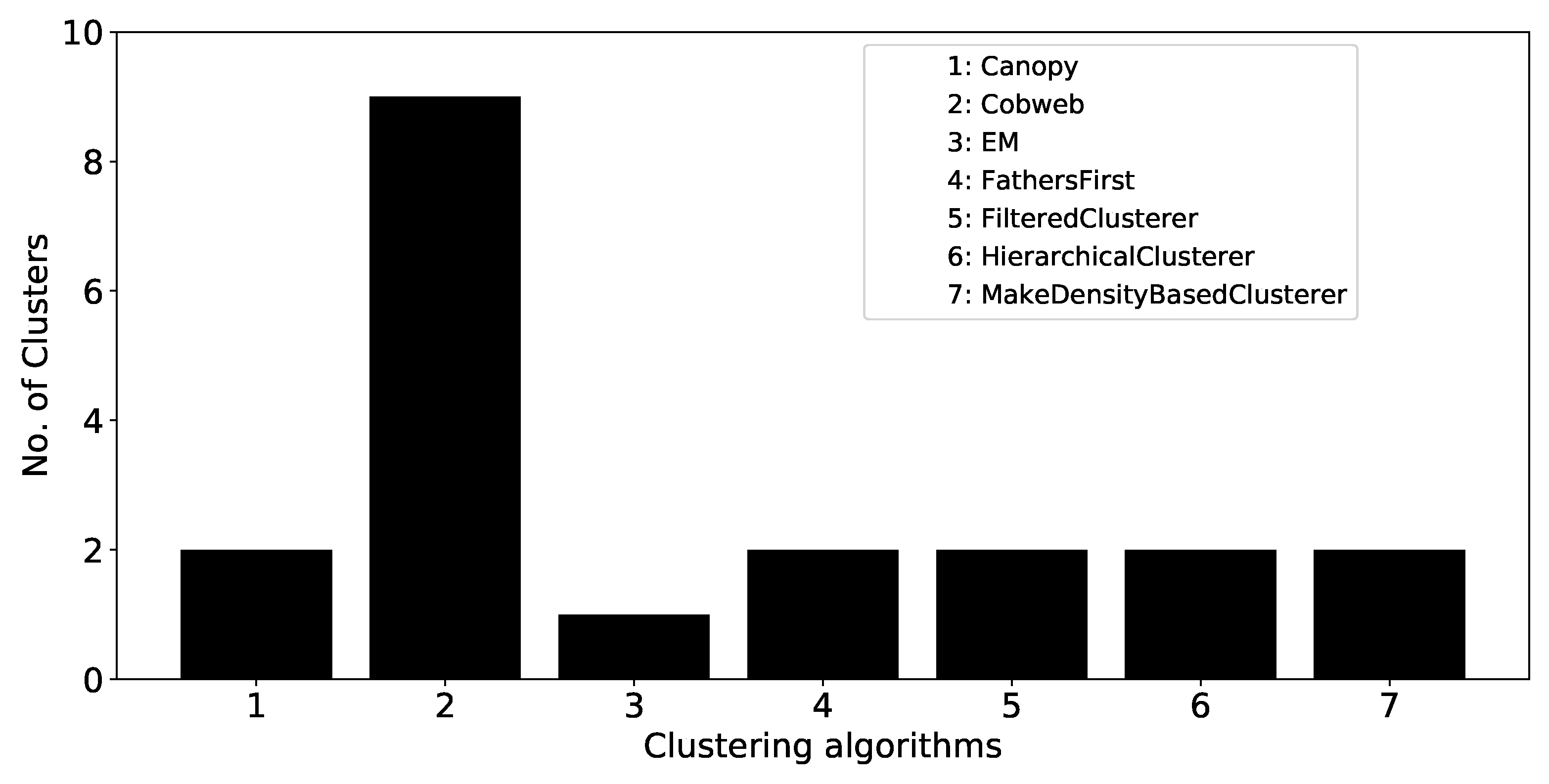
  • Canopy ([36]), an un-grouped pre-clustering algorithm that partitions input data into proximity regions (canopies) in the form of hyperspheres.
  • Cobweb ([37,38]), a hierarchical grouping algorithm that organises observations using a sorting tree.
  • EM ([39]), a probabilistic grouping algorithm that assigns each observation with a probability distribution indicating the likelihood of belonging to each of the examined groups.
  • FartherstFirst algorithm ([40]), based on a sequence of points the first of which is selected arbitrarily while each successive point is as far as possible from the set of previously-selected points.
  • FilteredClusterer ([41]), an arbitrary clusterer on data that has been passed through an arbitrary filter the structure of which is based exclusively on the training data.
  • HierarchicalClusterer ([41]), a cluster analysis aiming to build a hierarchy of clusters using the agglomerative approach.
  • MakeDensityBasedClusterer ([41]), a metaclusterer wrapping clustering algorithms aiming to output a probability distribution and density.
  • K-means ([42]), one of the simplest unsupervised learning techniques aimed at dividing observations into k arrays in which each observation belongs to the array with the closest mean.

4.2. Neural Network for New Records’ Classification

The interrelated data of the dataset, as discussed in Section 3, presents each record as a multidimensional vector that consists of environmental and pest information. The sensor-based data research direction explored herein, apart from the key issue of grouping data by similarity (i.e., the clustering methodology proposed in Section 4.1), introduces more interesting research issues such as the management of collected data after the initial grouping. The issue is more pressing given the Big Data nature of the collected information as far as mostly their volume, but also their velocity and variety [43].
Having a set of predefined groupings/clusters makes the management and assignment of newly collected (interrelated) records much easier and more computationally efficient with classification approaches based on pattern recognition methods. In detail, following the initial process of cluster definition based on an initial adequate volume of data, classification approaches can then handle the assignment of new records on existing clusters. By use of performance measurements, new records could either be incorporated into existing clusters (if the classification’s performance is below a threshold) or indicate the necessity for cluster re-definition (if the classification’s performance is above the threshold). Thus, for a fixed location, wherein the microclimates indicate an increased degree of stability, by following the proposed methodology the continuous flow of records will gradually invoke the costly clustering process less and less and the classification approach more, all the while retaining the ability to organise records based on relevant attributes and not static characteristics such as their location.
Accordingly, we propose the use of a shallow neural network pattern recognition approach and especially a two-layer feed-forward network [44] for the classification of the multidimensional vectors of the dataset’s records into predefined clusters. The proposed methodology contains a number of hidden layer neurons, the size of which is an examination parameter.

5. Experimental Evaluation

To show the efficiency of the proposed methodologies and the feature vector, in this section a number of experiments are presented. The experimentation’s pre-processing, platform and datasets are also described, followed by the performance and qualitative analysis of the experimental results.

5.1. Experimental Setup & Data

5.1.1. Statistical Analysis Grouping

Data collection: Prior to using the data for the experiments, a pre-processing treatment of the data was performed. Initially, the sub-set of time periods in which all sensors had recorded measurements was identified, as, for technical reasons, data collection was not entirely consistent. For the purposes of this examination, the common time period selected was between 24 September 2018 and 8 October 2018. Subsequently, corrupted data were also removed from the data-set (i.e., the dates from 30 September 2018 to 2 October 2018).
Figure 2 and Figure 3 show the recorded temperature and humidity for selected sensors in the aforementioned common time period. The blue line indicates the actual data, while the red line shows the data after smoothing by use of overlapping rolling window mean.
Feature selection: In order to conduct the experiments, the collected environmental data were converted to the following set of numerical attributes:
  • Temperature
    • Minimum temperature of the time series.
    • Average temperature of the time series.
    • Maximum temperature of the time series.
    • Typical temperature deviation of the time series.
    • Absolute difference in maximum and minimum temperature.
    • Average growth rate from minimum daily temperature to maximum daily temperature.
    • Average rate of decrease from maximum daily temperature to local minimum daily temperature.
    • Average maximum daily temperature.
    • Average minimum daily temperature.
    • Average absolute difference between maximum and minimum daily temperature.
    • Average degree of similarity of daily temperature time series for "Beach" locations.
    • Average degree of similarity of daily temperature time series for "Hill" locations.
    • Average degree of similarity of daily temperature time series for "Valley" locations.
  • Humidity
    • Minimum humidity of the time series.
    • Mean humidity of the time series.
    • Maximum time series humor.
    • Typical moisture deviation of the time series.
    • Absolute difference in maximum and minimum humidity.
    • Average minimum daily humidity.
    • Average maximum daily humidity.
Feature vector extraction: Of the 20 aforementioned attributes, the final selection of the attributes for the creation of the vector was based on the evaluation of each attribute in terms of Information Gain, Correlation and the Information gain ratio relative to the Microclimate class, that is, the location type.
Observing the diagram of Figure 4, it is evident that 7 of the 20 original features have an information gain ratio of 1 while the remainder are 0. More specifically, these are:
  • Mean temperature of the time series.
  • Typical temperature deviation of the time series.
  • Average minimum daily temperature.
  • Average degree of similarity of daily temperature time series for “Beach” locations.
  • Average degree of similarity of daily temperature time series for “Hill” locations.
  • Average degree of similarity of daily temperature time series for “Valley” locations.
  • Mean humidity of the time series.
Figure 5 shows the value of each attribute by their correlation coefficient in regard to the “Microclimate” cluster class. As can be seen from the diagram, the seven attributes that showed the highest information gain ratio (see Figure 4) plus attribute 10 (“Average absolute difference between maximum and minimum daily temperatures”) have the highest correlation (greater than 0.5).
Finally, the diagram in Figure 6 shows the information gain of the candidate features for the feature vector. As shown in the diagram, the same seven characteristics as the diagram of Figure 4 show the greatest gain of information. Specifically, characteristic 11 provides the highest information gain (1.585), while the remaining six characteristics (2, 4, 9, 12, 13, 15) offer the same gain of information, 0.918. The remaining features do not provide any gain of information.
From the above analysis the characteristics selected for the composition of the feature vector are the following:
  • Average degree of similarity of daily temperature time series for “Beach” locations.
  • Average degree of similarity of daily temperature time series for “Hill” locations.
  • Average degree of similarity of daily temperature time series for “Valley” locations.
  • Average minimum daily temperature.
  • Mean humidity of the time series.
  • Mean temperature of the time series.
  • Typical temperature deviation of the time series.
In order to conduct the clustering experiments, the WEKA Machine Learning Platform [45] was used. For the K-Means algorithm, the number of clusters ranged from 2 to 3 and the Manhattan and Euclidean distance functions were examined.

5.1.2. NN-Based Classification

In the neural network (NN)-based classification experimentation using the shallow neural network pattern recognition approach, a two-layer feed-forward network architecture was used containing a varying number of hidden neurons in order to test the effect of the neuron availability. Moreover, the experimentation also included various alternatives as far as the division of the dataset into training, validation, and testing subsets is concerned. The performance evaluation was tested based on manually pre-selected microclimates and the ability of the network to assign records that had not been included in the training and validation processes at the appropriate microclimate during the testing phase.
The training function used was the Scaled Conjugate Gradient Backpropagation function which updates weight and bias values according to the scaled conjugate gradient method [46]. The performance function used was the minimising cross-entropy function (ranging in (0, 1) with close to zero values indicating no error) that applies heavy penalties on outputs that exhibit extreme inaccuracy and light penalty for close to correct classifications. Moreover, for each classification, the percentage of error, that is, the fraction of samples misclassified, was also calculated in order to provide a degree of effectiveness of the method.
Finally, it should be noted that for each of the parameters examined (number of neurons and division of the dataset), the resulting performance of the network was averaged over 10 runs due to the randomness in the division of the dataset into training, validation and testing subsets and in order to receive high quality results.
In order to conduct the NN-based classification experimentation, the software MATLAB [47] version “9.4.0.813654 (R2018a)” was used.

5.2. Experimental Results

5.2.1. Results from Statistical Analysis Grouping

Figure 7 shows the number of clusters the data were split into after applying the clustering algorithms (Canopy, Cobweb, EM, FarthersFirst, FilteredClusterer, HierarchicalClusterer, MakeDensityBasedClusterer). The majority of these algorithms split the examined locations into two clusters, while the EM algorithm grouped all nine locations into one cluster. Finally, the Cobweb algorithm assigned each location to its own cluster, namely nine.
Figure 8 shows the accuracy of correct clustering of the samples from the clustering algorithms used in our experiments. The lowest performance was attained by EM and Cobweb algorithms with 33% accuracy. The K-means algorithm had the best performance (89%), with k = 3 for both of the distance functions considered. The remaining algorithms had a similar performance, which was approx. 66%.

5.2.2. Results from NN-Based Classification

In order to test the NN-based classification, we initially tested the effect of the division of the dataset into training, validation and testing subsets. Figure 9 shows that the best results for both Cross-entropy and Percentage of error were achieved, with significant differentiation to other alternatives for the division with 60% training, 20% validation and 20% testing. Accordingly, the rest of the experimentation on the NN-based classification was done with this division ratio.
The next experiment focuses on the on the effect of the hidden neurons on Cross-entropy and Percentage of error. Figure 10 shows the results obtained for a variety of different hidden neurons’ values ranging from 1 to 10,000. The results indicate that the best result as far as cross-entropy is concerned is achieved for 1000 hidden neurons while the lowest percentage of error is achieved for 2500 hidden neurons, though cross-entropy’s difference between 1000 and 2500 hidden neurons is almost negligible.

5.3. Results’ Discussion

Based on the feature vector used and the experiments carried out, the performance evaluation of the statistical analysis’ grouping results indicates that, for algorithms automatically selecting the number of clusters for the available data, the selected locations can be separated into two microclimates, the “Valley” and “Beach - Hill,” a merger of the areas that belonged to the microclimates “Beach” and “Hill” based on our initial hypothesis. Nevertheless, given the option of 3 clusters, the K-means algorithm presents the best precision of correct cluster classification, significantly exceeding the performance of the other methods (89% to 66%). This discrepancy is attributed to the generality of the examined algorithms, the high correlation between “Beach” and “Hill” type measurements as well as the small number of locations and short time-span examined.
The results obtained by the NN-based classification exhibit two significant takeaways:
  • The variability of the division of the dataset into training, validation and testing subsets, as shown in Figure 10, affects both Cross-entropy and Percentage of error of the classification process but the effect is of limited breadth. For all variations tested, the difference between min and max values were 4.1% for the Cross-entropy and 6.4% for the Percentage of error. In contrast, the variability of the hidden neurons showed a rather significant effect with the difference between min and max values being 64.4% for the Cross-entropy and 23% for the Percentage of error. It is thus crucial for the effectiveness of the proposed methodology to identify the size of hidden neurons that keep both Cross-entropy and Percentage of error at their lowest values.
  • The performance of the classification in absolute values was shown to be high based on both the Cross-entropy and Percentage of error results obtained. Qualitatively, Cross-entropy assesses how accurate a model is at predicting some test data and thus comparing the 2 distributions which get their minimal value when the distributions are equal. The trend shown in Figure 10, of Cross-entropy minimising up until 2500 hidden neurons, indicates the progressive and very close equal case of the 2 distributions and thus the accuracy of the NN model in predicting the test data. The Percentage of errors is similarly inline with the Cross-entropy results as both metrics are approximately over 85% of the best scenario.
The high performance of the collected results’ clustering and classification obtained herein, in combination with the results obtained by Kalamatianos and Avlonitis [17], constitute a promising direction, when viewed as complementary, for the identification of microclimates related to the olive fruit-fly’s life-cycle that may subsequently be modelled into accurate population dynamics predictions of the olive fruit fly.

6. Conclusions

In this work, methods for the identification of localised environmental/climate conditions (microclimates) related to the life-cycle of the olive fruit fly are proposed. The two methods employed herein—the statistical analysis and the Neural Network based classification—are complementary with one another, aiming to provide the required initial clustering and the subsequent classification of sensory records into the existing clusters with focus on efficiency and effectiveness.
Based on interrelated environmental and pest data collected from olive groves in North Western Kerkyra, Greece, the two methods were applied and extensive experimentation indicated very promising results for both parts of the proposed methodology. Qualitative evaluation of the results obtained indicated the applicability of the proposed method for real-life uses.
Future plans for this research domain will focus on more detailed and diverse environmental measurements (location and attribute wise) as well as more frequent pest measurements that are based on smart-traps that minimise the manual interaction as much as possible. Given the larger volume of data aimed for, methods that expand from the shallow Neural Networks presented here to their deep equivalent are also part of future plans.

Author Contributions

All authors contributed equally to the work.

Funding

The present research was carried out by the Ionian University of the Ionian Islands, Greece within the framework of the project “Olive Observer” of the ROP “Ionia Nisia 2014-2020” co-funded by the European Union (ERDF) and Greece.

Conflicts of Interest

The authors declare no conflict of interest.

References

  1. Bass, M.A.; Wakefield, L.; Kolasa, K. Community Nutrition and Individual Food Behavior; Burgess Pub. Co.: Minneapolis, MN, USA, 1979. [Google Scholar]
  2. Parsa, S.; Morse, S.; Bonifacio, A.; Chancellor, T.C.; Condori, B.; Crespo-Pérez, V.; Hobbs, S.L.; Kroschel, J.; Ba, M.N.; Rebaudo, F.; et al. Obstacles to integrated pest management adoption in developing countries. Proc. Natl. Acad. Sci. USA 2014, 111, 3889–3894. [Google Scholar] [CrossRef] [PubMed] [Green Version]
  3. Boccaccio, L.; Petacchi, R. Landscape effects on the complex of Bactrocera oleae parasitoids and implications for conservation biological control. Biocontrol 2009, 54, 607. [Google Scholar] [CrossRef]
  4. Lamichhane, J.R.; Dachbrodt-Saaydeh, S.; Kudsk, P.; Messéan, A. Toward a reduced reliance on conventional pesticides in European agriculture. Plant Disease 2016, 100, 10–24. [Google Scholar] [CrossRef] [PubMed]
  5. Karydis, I.; Gratsanis, P.; Semertzidis, C.; Avlonitis, M. WebGIS Design & Implementation for Pest Life-cycle & Control Simulation: The Case of Olive-fruit Fly. In Proceedings of the International Conference on Information and Communication Technologies in Agriculture, Food and Environmentp, Corfu Island, Greece, 19–22 September 2013; pp. 526–529. [Google Scholar]
  6. Kalamatianos, R.; Kermanidis, K.; Karydis, I.; Avlonitis, M. Treating stochasticity of olive-fruit fly’s outbreaks via machine learning algorithms. Neurocomputing 2018, 280, 135–146. [Google Scholar] [CrossRef]
  7. Kalamatianos, R.; Bouchagier, P.; Avlonitis, M. Modeling the effect of olive fruit bearing percentage on Bactrocera oleae stochastic dispersion. J. Agric. Informat. 2018, 9, 12–21. [Google Scholar] [CrossRef]
  8. Eurostat. Agri-Environmental Indicator—Cropping Patterns, Data from March 2017; Eurostat: Luxembourg, Luxembourg, 2017. [Google Scholar]
  9. Fogher, C.; Busconi, M.; Sebastiani, L.; Bracci, T. Olive Genomics. In Olives and Olive Oil in Health and Disease Prevention; Preedy, V.R., Watson, R.R., Eds.; Academic Press: San Diego, CA, USA, 2010; Chapter 2; pp. 17–24. [Google Scholar] [CrossRef]
  10. Agriculture and Rural Development. EU Agricultural Outlook: Wine, Olive Oil and Fruits & Vegetable Exports to Grow; European Union: Brussels, Belgium, 19 December 2017. [Google Scholar]
  11. Haniotakis, G.E. Olive pest control: Present status and prospects. IOBC WPRS Bull. 2005, 28, 1–9. [Google Scholar]
  12. Tsitsipis, J. Effect of constant temperature on the eggs of the olive fruit fly, Dacus oleae (Diptera, Tephritidae). Ann. Zool. Ecol. Anim. 1977, 9, 133–139. [Google Scholar]
  13. Tsitsipis, J.A. Effect of constant temperatures on larval and pupal development of olive fruit flies reared on artificial diet. Environ. Entomol. 1980, 9, 764–768. [Google Scholar] [CrossRef]
  14. Wang, X.G.; Johnson, M.W.; Daane, K.M.; Opp, S. Combined effects of heat stress and food supply on flight performance of olive fruit fly (Diptera: Tephritidae). Ann. Entomol. Soc. Am. 2009, 102, 727–734. [Google Scholar] [CrossRef]
  15. Broufas, G.; Pappas, M.; Koveos, D. Effect of relative humidity on longevity, ovarian maturation, and egg production in the olive fruit fly (Diptera: Tephritidae). Ann. Entomol. Soc. Am. 2009, 102, 70–75. [Google Scholar] [CrossRef]
  16. Pappas, M.; Broufas, G.; Koufali, N.; Pieri, P.; Koveos, D. Effect of heat stress on survival and reproduction of the olive fruit fly Bactocera (Dacus) oleae. J. Appl. Entomol. 2011, 135, 359–366. [Google Scholar] [CrossRef]
  17. Kalamatianos, R.; Avlonitis, M. Microclimates and their Stochastic Effect on Olive Fruit Fly Evolution: Modeling and Simulation. In Proceedings of the 8th International Conference on Information and Communication Technologies in Agriculture, Food and Environment (HAICTA), Chania, Greece, 21–24 September 2017; Volume 2030. [Google Scholar]
  18. Cantlon, J.E. Vegetation and Microclimates on North and South Slopes of Cushetunk Mountain, New Jersey. Ecol. Monogr. 1953, 23, 241–270. [Google Scholar] [CrossRef]
  19. Van Cooten, S.; Barbe, D.; McCorquodale, D.; Cothren, D. Identification of precipitation microclimates and rainfall trends across the Lake Pontchartrain Basin of southeast Louisiana. In Proceedings of the Mississippi River Climate and Hydrology Conference, New Orleans, LA, USA, 13–17 May 2002. [Google Scholar]
  20. Shafieiyoun, E. Identification of Micro-Climates of Isfahan City and its Effect on Air Temperature, Relative Air Humidity and Reference Crop Evapotranspiration. In Proceedings of the 3rd ScienceOne International Conference on Environmental Sciences, Dubai, United Arab Emirates, 21–23 January 2014. [Google Scholar]
  21. Dimoudi, A.; Kantzioura, A.; Zoras, S.; Pallas, C.; Kosmopoulos, P. Investigation of urban microclimate parameters in an urban center. Energy Build. 2013, 64, 1–9. [Google Scholar] [CrossRef]
  22. Wong, N.H.; Jusuf, S.K. Study on the microclimate condition along a green pedestrian canyon in Singapore. Archit. Sci. Rev. 2010, 53, 196–212. [Google Scholar] [CrossRef]
  23. Stabler, L.B.; Martin, C.A.; Brazel, A.J. Microclimates in a desert city were related to land use and vegetation index. Urban For. Urban Green. 2005, 3, 137–147. [Google Scholar] [CrossRef]
  24. Shahrestani, M.; Yao, R.; Luo, Z.; Turkbeyler, E.; Davies, H. A field study of urban microclimates in London. Renew. Energy 2015, 73, 3–9. [Google Scholar] [CrossRef] [Green Version]
  25. Zhang, Y.; Mahrer, Y.; Margolin, M. Predicting the microclimate inside a greenhouse: An application of a one-dimensional numerical model in an unheated greenhouse. Agric. For. Meteorol. 1997, 86, 291–297. [Google Scholar] [CrossRef]
  26. Avissar, R.; Mahrer, Y. Verification study of a numerical greenhouse microclimate model. Trans. ASAE 1982, 25, 1711–1720. [Google Scholar] [CrossRef]
  27. Wang, S.; Boulard, T. Predicting the microclimate in a naturally ventilated plastic house in a Mediterranean climate. J. Agric. Eng. Res. 2000, 75, 27–38. [Google Scholar] [CrossRef]
  28. Kearney, M.R.; Shamakhy, A.; Tingley, R.; Karoly, D.J.; Hoffmann, A.A.; Briggs, P.R.; Porter, W.P. Microclimate modelling at macro scales: A test of a general microclimate model integrated with gridded continental-scale soil and weather data. Methods Ecol. Evol. 2014, 5, 273–286. [Google Scholar] [CrossRef]
  29. Holmes, R.; Nelson Dingle, A. The relationship between the macro-and microclimate. Agric. Meteorol. 1965, 2, 127–133. [Google Scholar] [CrossRef]
  30. Kearney, M.R.; Isaac, A.P.; Porter, W.P. Microclim: Global estimates of hourly microclimate based on long-term monthly climate averages. Sci. Data 2014, 1, 140006. [Google Scholar] [CrossRef] [PubMed]
  31. Kalamatianos, R.; Avlonitis, M.; Stravoravdis, S. Complex networks and simulation strategies: An application to olive fruit fly dispersion. In Proceedings of the 2015 6th International Conference on Information, Intelligence, Systems and Applications (IISA), Corfu, Greece, 6–8 July 2015; pp. 1–6. [Google Scholar]
  32. Vossen, P.; Varel, L.G.; Alexandra, D. Olive Fruit Fly; Technical Report; University of California Cooperative Extension: Sonoma County, CA, USA, 2004; Available online: http://cenapa.ucanr.edu/files/52578.pdf (accessed on 20 April 2019).
  33. Kounatidis, I.; Papadopoulos, N.; Mavragani-Tsipidou, P.; Cohen, Y.; Tertivanidis, K.; Nomikou, M.; Nestel, D. Effect of elevation on spatio-temporal patterns of olive fly (Bactrocera oleae) populations in northern Greece. J. Appl. Entomol. 2008, 132, 722–733. [Google Scholar] [CrossRef]
  34. Ruesink, W.G.; Kogan, M. The quantitative basis of pest management: Sampling and measuring. In Introduction to Insect Pest Management; Wiley: New York, NY, USA, 1994; pp. 355–391. [Google Scholar]
  35. Kalamatianos, R.; Karydis, I.; Doukakis, D.; Avlonitis, M. DIRT: The Dacus Image Recognition Toolkit. J. Imaging 2018, 4, 129. [Google Scholar] [CrossRef]
  36. McCallum, A.; Nigam, K.; Ungar, L.H. Efficient clustering of high-dimensional data sets with application to reference matching. In Proceedings of the Sixth ACM SIGKDD International Conference on Knowledge Discovery and Data Mining, Boston, MA, USA, 20–23 August 2000; pp. 169–178. [Google Scholar]
  37. Fisher, D.H. Knowledge acquisition via incremental conceptual clustering. Mach. Learn. 1987, 2, 139–172. [Google Scholar] [CrossRef]
  38. Fisher, D.H. Improving Inference through Conceptual Clustering; AAAI: Menlo Park, CA, USA, 1987; Volume 87, pp. 461–465. [Google Scholar]
  39. Dempster, A.P.; Laird, N.M.; Rubin, D.B. Maximum likelihood from incomplete data via the EM algorithm. J. R. Stat. Soc. Ser. B (Methodol.) 1977, 39, 1–22. [Google Scholar] [CrossRef]
  40. Hochbaum, D.S.; Shmoys, D.B. A best possible heuristic for the k-center problem. Math. Oper. Res. 1985, 10, 180–184. [Google Scholar] [CrossRef]
  41. Witten, I.H.; Frank, E.; Hall, M.A.; Pal, C.J. Data Mining: Practical Machine Learning Tools and Techniques; Morgan Kaufmann: Burlington, MA, USA, 2016. [Google Scholar]
  42. Forgy, E.W. Cluster analysis of multivariate data: Efficiency versus interpretability of classifications. Biometrics 1965, 21, 768–769. [Google Scholar]
  43. Laney, D. 3D data management: Controlling data volume, velocity and variety. META Group Res. Note 2001, 6, 1. [Google Scholar]
  44. Svozil, D.; Kvasnicka, V.; Pospichal, J. Introduction to multi-layer feed-forward neural networks. Chemom. Intell. Lab. Syst. 1997, 39, 43–62. [Google Scholar] [CrossRef]
  45. Hall, M.; Frank, E.; Holmes, G.; Pfahringer, B.; Reutemann, P.; Witten, I.H. The WEKA data mining software: An update. ACM SIGKDD Explor. Newsl. 2009, 11, 10–18. [Google Scholar] [CrossRef]
  46. Møller, M.F. A scaled conjugate gradient algorithm for fast supervised learning. Neural Netw. 1993, 6, 525–533. [Google Scholar] [CrossRef]
  47. MATLAB and Statistics Toolbox. 9.4.0.813654 (R2018a); The MathWorks Inc.: Natick, MA, USA, 2018; Available online: https://www.mathworks.com (accessed on 20 April 2019).
Figure 1. Locations of selected sensors. (Map data: Google, SIO, NOAA, U.S. Navy, NGA and GEBCO).
Agronomy 09 00337 g001
Figure 2. Recorded temperatures for selected locations of “Hill” type.
Agronomy 09 00337 g002
Figure 3. Recorded humidity for selected locations of “Valley” type.
Agronomy 09 00337 g003
Figure 4. Information gain ratio of all examined attributes relative to the Microclimate class.
Agronomy 09 00337 g004
Figure 5. Correlation of all examined attributes relative to the Microclimate class.
Agronomy 09 00337 g005
Figure 6. Information gain of all examined attributes relative to the Microclimate class.
Agronomy 09 00337 g006
Figure 7. Number of clusters different clustering algorithms grouped the supplied data.
Agronomy 09 00337 g007
Figure 8. Precision of correct cluster classification for different clustering algorithms.
Agronomy 09 00337 g008
Figure 9. Cross-entropy and Percentage of error for varying divisions of the dataset into training, validation, and testing subsets.
Agronomy 09 00337 g009
Figure 10. Cross-entropy and Percentage of error for varying hidden neurons.
Agronomy 09 00337 g010
Table 1. Selected data collection locations.
Location LabelAltitude (m)LatitudeLongitude
Beach
1Agios Georgios Pagon3839.7055810519.68224189
2Afionitika2439.73725119.654854
3Avliotes10639.7802730619.65994629
Hill
4Agios Athanasios21239.724306219.7172308
5Dafni14439.7288817319.7024659
6Rachtades13539.7514310419.69852521
Valley
7Gavrades5839.7398666519.71007243
8Psathilas3939.7453917819.71654322
9Kounavades3939.7568838519.69359849

