Real-Time Semantic Reconstruction and Semantically Constrained Path Planning for Agricultural Robots in Greenhouses

Abstract

To address perception and navigation challenges in precision agriculture caused by GPS signal loss and weakly structured environments in greenhouses, this study proposes an integrated framework for real-time semantic reconstruction and path planning. This framework comprises three core components: First, it introduces a semantic segmentation method tailored for greenhouse environments, enhancing recognition accuracy of key navigable areas such as furrows. Second, it designs a visual-semantic fusion SLAM point cloud reconstruction algorithm and proposes a semantic point cloud rasterization method. Finally, it develops a semantic-constrained A* path planning algorithm adapted for semantic maps. We collected a segmentation dataset (1083 images, 4 classes) and a reconstruction dataset from greenhouses in Shanghai. Experiments demonstrate that the segmentation algorithm achieves 95.44% accuracy and 87.93% mIoU, with a 3.9% improvement in furrow category recognition accuracy. The reconstructed point cloud exhibits an average relative error of 7.37% on furrows. In practical greenhouse validation, single-frame point cloud fusion took approximately 0.35 s, while path planning was completed in under 1 s. Feasible paths avoiding crops were successfully generated across three structurally distinct greenhouses. Results demonstrate that this framework can stably and in real-time accomplish semantic mapping and path planning, providing effective technical support for digital agriculture.

1. Introduction

In recent years, vegetable greenhouses have gained widespread adoption in modern agriculture due to their controllable internal environments and high yields. However, the enclosed spaces and high planting densities within greenhouses make vegetable plants susceptible to competition from weeds. Manual weeding is labor-intensive, costly, and inefficient, creating an urgent need for automated weeding robots with autonomous sensing capabilities [1,2].

Existing weeding robot products, such as Carbon Robotics [3], TerraSentia [4], EcoRobotix [5], and AVO [6], have achieved breakthroughs in automated laser, mechanical, and chemical weeding methods. However, these systems rely on global satellite navigation systems and drones to construct global maps and plan operational paths for navigation and environmental understanding. Constrained by the enclosed roof structure of vegetable greenhouses, this global map acquisition method is difficult to implement within such environments. Furthermore, traditional geometric maps can only distinguish simple obstacles and cannot accurately determine whether crops are damaged in the confined space of greenhouses. This geometry-based approach to scene understanding struggles to meet the operational safety and precision requirements of complex agricultural environments.

To achieve higher-level environmental understanding, semantic segmentation and object detection techniques have been introduced into agricultural scene perception tasks for identifying scene elements such as crops, roads, obstacles, and weeds. Existing research has applied semantic information to row detection and area recognition in agricultural scenes. For instance, Diao et al. [7] proposed the ASPP-YOLOV8S network for crop canopy detection, Liu et al. [8] designed an enhanced MS-ERFNet architecture to improve segmentation performance in farmland scenes, and Bah et al. [9] developed the end-to-end CRowNet network for crop row recognition. Other studies have utilized semantic segmentation algorithms to locate obstacles in complex agricultural environments [10,11]. However, existing methods are largely confined to two-dimensional images, failing to effectively map semantic information into three-dimensional space. Consequently, they cannot construct detailed semantic maps suitable for path planning tasks.

In agricultural robot navigation tasks where direct access to global maps is challenging, Simultaneous Localization and Mapping (SLAM) technology can construct the scene’s global geometric information by collecting local data. Since the map structure of soil-based greenhouses dynamically changes during vegetable sowing, growth, irrigation, and other stages, the map must be reconstructed before each operation. Semantic information about the scene must be integrated into the map to precisely delineate navigable boundaries. Laser-based SLAM methods can directly generate point cloud maps, but the unstructured nature of point cloud data limits efficient semantic information integration [12,13]. Visual SLAM technologies, however, acquire scene point clouds through image reprojection, enabling semantic information embedding. For instance, Yan et al. [14] proposed a multi-sensor fusion visual SLAM system achieving semantic reconstruction in complex facility agriculture environments; Chen et al. [15] completed global point cloud reconstruction for orchard scenes using stereo vision. In recent years, research has also integrated Transformer-based semantic segmentation techniques with SLAM tasks, yielding algorithms such as DDETR-SLAM [16]. However, such approaches remain limited in agricultural applications. Additionally, studies have attempted to fuse radar-derived geometric information with visually acquired semantic data for agricultural scene reconstruction [17,18,19], but current studies primarily focus on local perception within the immediate forward workspace, without systematic application to global semantic point cloud map construction. Currently, there remains a lack of lightweight, semantically enhanced reconstruction methods tailored for soil-based vegetable greenhouse scenarios that can generate semantically rich maps suitable for operational path planning while maintaining real-time performance.

Previous studies have proposed various optimization algorithms for path planning in agricultural scenarios, enabling efficient computation of shortest paths between target points in environments with known obstacle distributions. Examples include Wei et al.’s [20] multi-task constrained convex optimization framework for path planning around planting pots, as well as Zhang et al.’s [21] and Wang et al.’s [22] improved A* algorithms incorporating Bézier curves or fuzzy dynamic window methods algorithm for obstacle avoidance path planning in agricultural environments. Current research primarily focuses on path planning for navigating scenes with clearly defined obstacles, lacking adaptation to semantic information. Path planning algorithms that determine passable areas based on semantic judgments have also been studied in the agricultural domain. For instance, some research [23,24] constructs global crop row distribution models by processing drone imagery to achieve global coverage path planning for agricultural vehicles. Other studies [25,26] utilize low-altitude remote sensing technology to segment detailed distribution areas of crops and weeds, planning avoidance paths accordingly. Existing semantic path planning largely relies on global scenes constructed via low-altitude remote sensing, with semantic information primarily used for simple passable area segmentation—similar to occupancy processing in traditional raster maps. This approach fails to fully account for the interactive relationships between semantic information and robotic components, limiting its adaptability in complex indoor operational scenarios. For soil-cultivated vegetable greenhouse environments like those addressed in this paper, there remains a lack of a suitable passable space definition method. Furthermore, the maps we construct, which contain semantic hierarchical information such as crop distribution locations, currently lack a path planning algorithm that can closely adapt to them.

To address the challenges of pixel-level semantic information acquisition, semantic-scene point cloud fusion, and semantic-aware path generation in facility agriculture navigation, we propose a real-time semantic reconstruction and path planning algorithm framework tailored for facility operation scenarios.

The main contributions of this study include the following:

(1)

To address the issue of class imbalance in soil-based greenhouse environments, we propose a semantic segmentation method that applies a mixed loss function to the Segformer network, significantly improving segmentation accuracy for narrow furrow terrain.

(2)

To address the challenge of acquiring global semantic maps in multi-span greenhouses, a visual-semantic fusion SLAM point cloud reconstruction algorithm is proposed. A semantic point cloud rasterization method based on semantic feature vectors is introduced, enabling rapid global map construction.

(3)

To address the challenge of planning valid operational paths on the global semantic map of greenhouses, a semantic-constrained A* path planning algorithm is designed. This algorithm explicitly simulates the interactive characteristics of weeding robots, enabling the generation of operational paths that meet agricultural requirements.

The open-source code for this project is published at https://github.com/xxscfo/Semantic-Point-Cloud-Reconstruction-and-Path-Planning-Algorithm-for-Greenhouse-Scenarios (accssed on 9 November 2025).

2. Materials and Methods

2.1. Experimental Facilities and Data Preparation

2.1.1. Experimental Site

The experimental data for this study were collected at the Pujiang Green Valley Low-Carbon Agricultural Base of Shanghai Jiao Tong University (31.05° N, 121.50° E) in Shanghai, China. Data acquisition and algorithm validation experiments are conducted in an indoor soil-based greenhouse environment for Chinese cabbage cultivation. Figure 1 illustrates the multi-span greenhouse vegetable production environment targeted in this research.

Figure 1. Vegetable greenhouse scene.

The vegetable greenhouse complex features a rectangular layout measuring approximately 33 m in length and either 56 m or 40 m in width. A paved path (approximately 2 m wide) runs transversely near the entrance to facilitate robotic access; the remaining area is divided into multiple planting zones separated by fixed steel support poles. The planting surface is approximately 1.1 m wide, with furrows about 30 cm wide, separated by a height difference of roughly 15 cm. Due to variations in soil properties and crop growth periods, the planting surface height may exhibit a height difference of ±10 cm relative to the paved path. The planting zones extend from the paved path to the opposite wall of the structure. Because of this layout constraint, the robot can only execute turns on the paved path. Manual preparation of the planting surface is required before each planting cycle, and watering may cause soil displacement or subsidence. This results in an inconsistent distribution of planting areas across different greenhouses, creating an unstructured environment for robot navigation.

2.1.2. Experimental Platform

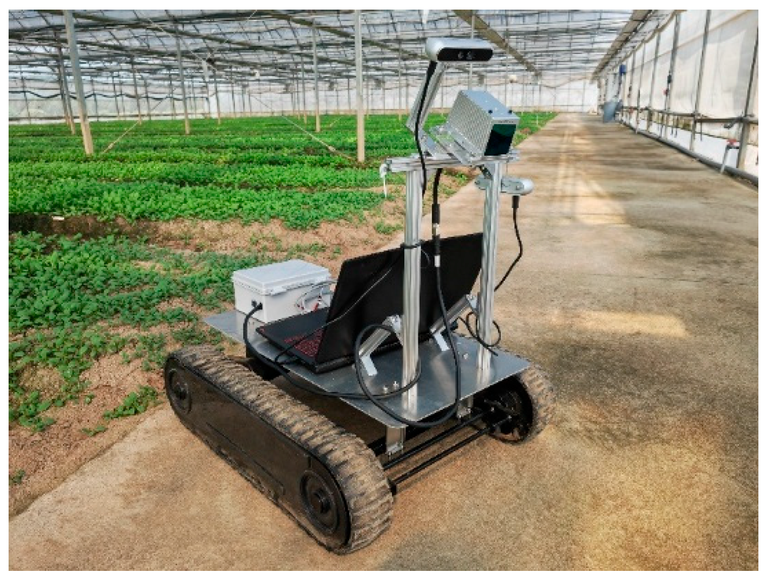
The experimental platform employed in this study utilizes a self-designed sampling crawler vehicle, as shown in Figure 2, equipped with an 80 cm × 60 cm tracked chassis. This vehicle utilizes a lithium battery with a capacity of approximately 25 Ah as its power source, delivering an output voltage of 12 V to supply power to both the chassis and the radar. The combined power consumption of these two components is approximately 45 W. Testing has confirmed that the power supply can sustain continuous operation of the sampling vehicle for over 3 h, which is sufficient to complete sampling and experimental tasks. It should be noted that this sampling vehicle is solely intended for collecting data required for this study (including semantic segmentation datasets and scene reconstruction datasets) and for verifying algorithm effectiveness and real-time performance via its onboard computer. It is not a prototype for long-term use as a laser-based weeding robot in agricultural settings.

Figure 2. Sampling crawler vehicle.

The sampling vehicle is equipped with an Inter RealSense d455f camera to capture RGB images and depth maps of vegetable greenhouses for segmentation and reconstruction. The RGB image capture resolution is 640 × 480 pixels with 8-bit color depth per channel, a field of view (FOV) of 90° × 65°, and a frame rate of 30 fps. Depth resolution is 640 × 480 pixels at 30fps, with temporal noise ≤ 1% and depth error ≤ 2% within 6 m. The minimum effective depth range is 58 cm, FOV is 87° × 58°, and depth maps are saved in z16 format. The camera’s built-in hole-filling filter is applied during capture to smooth depth noise. We calibrated the depth and RGB fields of view using the Realsense SDK to maintain precise alignment, ensuring each pair of RGB and depth images was temporally and spatially aligned during data acquisition. The camera was positioned approximately 60 cm above the ground at a 30° downward tilt. Crops and ground surfaces ranged from 0.8 m to 5 m from the camera, enabling acquisition of ground and vegetable field imagery within the immediate vicinity of the tracked vehicle. This data reconstructs the ground environment traversed during robotic navigation.

The sampling vehicle utilizes a PC as its onboard computing unit, secured to the tracked chassis via a custom-designed restraint frame to prevent bouncing or shifting during rough terrain. Protective covers are installed over the keyboard, ports, and other components to shield the equipment from dust damage. This PC is equipped with an NVIDIA RTX 4060 graphics card (8GB VRAM), an Intel i9-13900H processor, and 16 GB of memory. Running Ubuntu 20.04 and the ROS Noetic system, it can collect image data and run semantic reconstruction algorithms in real time. The PC connects to the depth camera via a USB 3.1 interface supporting 5Gbps transfer rates, enabling real-time scene reconstruction algorithm execution to validate effectiveness and capture runtime metrics.

Additionally, the experimental platform is equipped with a Livox Mid 70 LiDAR system (Livox Technology Company Limited, Shenzhen City, Guangdong Province, China). By synthesizing radar point cloud data from the collected point cloud, it enables both qualitative comparisons of geometric structures and dimensional comparisons at specific locations. This approach evaluates the quality of reconstructed point clouds obtained using depth cameras. The field of view (FOV) is a 70.4° circular area, with a range of 90 m at 10% reflectivity and an operating voltage of 12 V.

2.1.3. Dataset Preparation

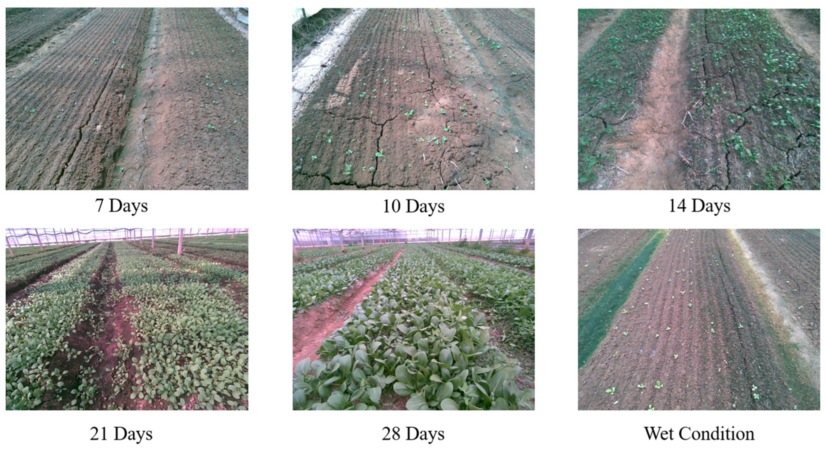
To evaluate our semantic segmentation model, we captured 640 × 480-pixel RGB images using Realsense D455f cameras (Intel, Santa Clara, CA, USA) in five greenhouse structures. This data collection spanned two months, encompassing vegetable field data at growth stages of 7 days, 10 days, 14 days, 21 days, and 28 days. Data collection occurred during morning, noon, and afternoon sessions, including lighting conditions on overcast and rainy days. Due to poor nighttime supplemental lighting in the greenhouses, which caused significant errors in the depth camera, we excluded nighttime working environments. Ultimately, we collected 1083 images from the multi-span greenhouses, capturing vegetable beds, furrows, concrete pathways, and surrounding environmental facilities (Figure 3).

Figure 3. Types of images included in the split dataset.

We defined four categories (planting surface, furrow, paved path, and background) for pixel-level semantic annotation. Data annotation was collaboratively performed by three agricultural experts using the LabelMe tool. All annotations were converted into labeled images in PNG format, with each pixel’s grayscale value defined as 0–3 to correspond to its assigned category. Given the limited initial dataset size, we employed a 5× data augmentation strategy during training to enhance the model’s robustness. The specific data augmentation operations include the following: (1) Geometric transformations: horizontal flipping with 0.5 probability, random rotation within ±90°, and random scaling within the range [0.8, 1.2]. (2) Randomly adjusting image brightness (range [0.8, 1.2]), contrast ([0.9, 1.1]), and saturation ([0.9, 1.1]) to simulate lighting variations across different times. We randomly partitioned 1083 images into training (758 images), validation (217 images), and test (108 images) sets at a ratio of 7:2:1. During partitioning, we strictly ensured that data from the same greenhouse and identical growth stages were assigned to the same set, thereby preventing data leakage.

For the dataset used in scene reconstruction, we collected data from three connected greenhouses, saved in rosbag format. To prevent data leakage caused by overlapping semantic segmentation data with training data, we avoided collecting data from cabbage crops planted in the same batch as the semantic data collection. Instead, we waited for the next planting cycle, allowing the crops to grow to a suitable stage before collecting data. Furthermore, among the three connected greenhouses used for experimentation, two were previously used for semantic segmentation data collection, while the third had never been used for data collection before. Each scene underwent at least three data collection sessions to ensure stable algorithm performance across all scenarios.

2.2. Algorithm for Real-Time Semantic Reconstruction and Task Path Generation in Facility Greenhouses

2.2.1. Algorithm Framework

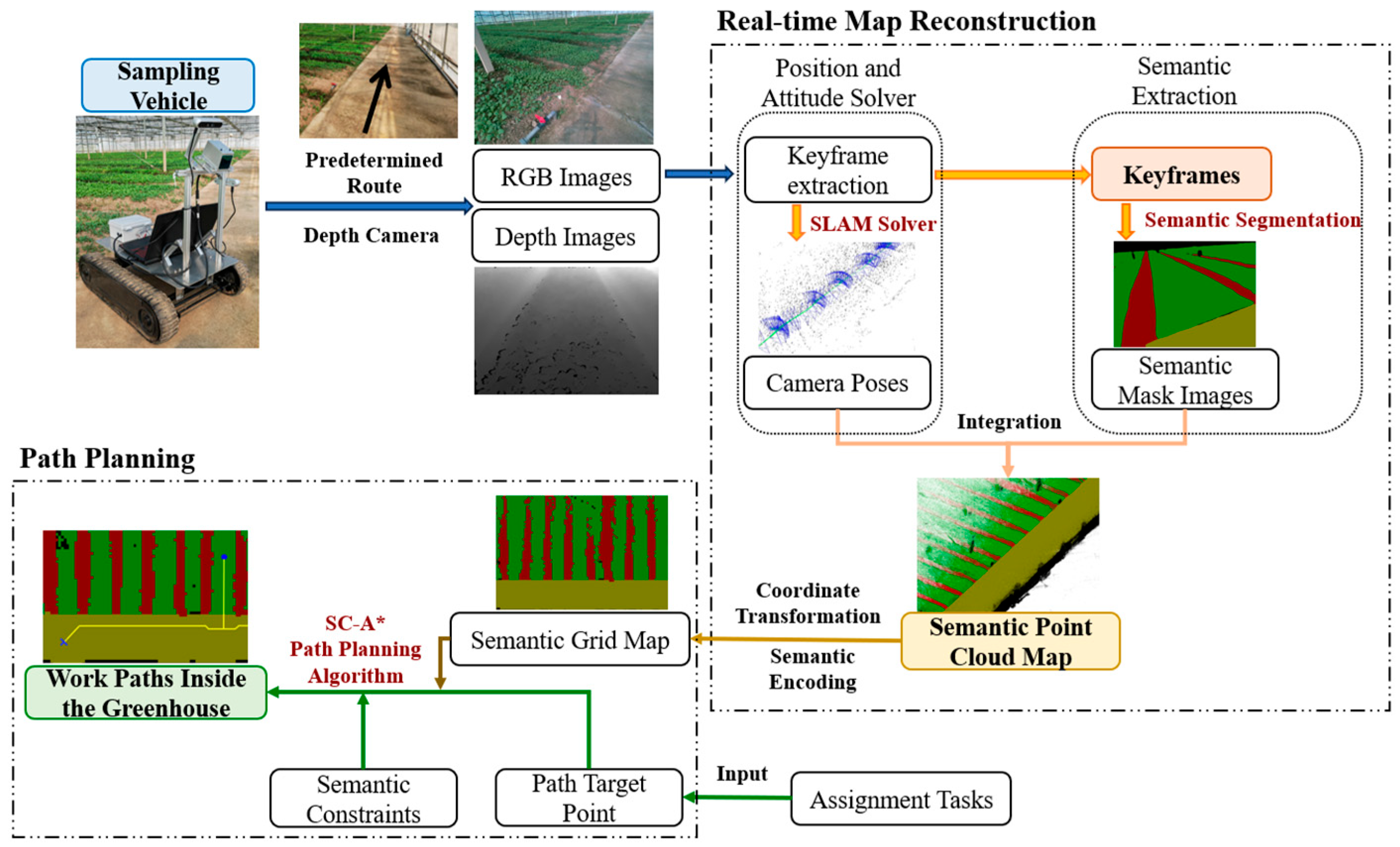
The structure of the real-time semantic reconstruction and task path planning system for facility greenhouses is shown in Figure 4. First, in the experimental platform section, the sampling vehicle is equipped with a power supply, depth camera, and PC. It travels along a predetermined route on the paved path, using the camera to capture RGB images and depth images of the scene. The PC performs spatiotemporal alignment between the two and provides the aligned data as input to the subsequent algorithm section.

Figure 4. Algorithm framework architecture for real-time semantic reconstruction and path planning in greenhouse facilities.

The algorithm section is divided into real-time mapping and path planning modules based on their execution sequence. Within the real-time map reconstruction module, the semantic point cloud of the scene is first acquired. At this stage, the pose estimation based on visual SLAM and the semantic extraction algorithm based on Segformer operate in tandem. The visual SLAM component utilizes feature matching from RGB images to generate a list of keyframes. Combined with depth images, it employs the Bundle Adjustment method to solve for the real-time poses of each keyframe. Simultaneously, the semantic extraction algorithm runs in parallel, accessing the acquired keyframes to perform pixel-level semantic segmentation on each frame, thereby obtaining per-pixel semantic information. Subsequently, this semantic information is fused with pose information and depth information to generate a 3D point cloud map of the scene containing semantic details. By performing coordinate transformation and raster semantic encoding on the generated semantic point cloud, the reconstructed 3D semantic map is converted into a semantic raster map to adapt to path planning tasks. In path planning, the generated semantic raster map serves as input, with task objectives inputted into the system as path grid coordinates within the scene. Considering the operational characteristics of weeding robots, a semantic constraint-optimized A* algorithm is applied to derive the SC-A* (Semantically Enhanced A*) path planning algorithm, ultimately achieving operational path planning within soil-based greenhouse environments. The following sections describe the principles of the Segformer-based semantic segmentation algorithm, the point cloud and raster map reconstruction algorithm based on visual SLAM methods, and the SC-A* algorithm.

2.2.2. Lightweight Semantic Segmentation for Greenhouse Scenes Based on SegFormer

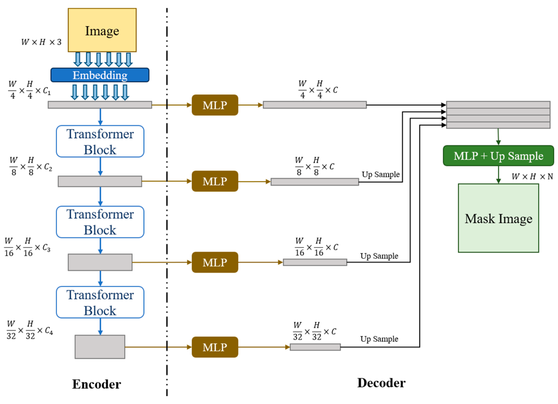
The semantic information within agricultural greenhouses primarily encompasses cultivated crop areas, ridges and furrows, pathways, and miscellaneous objects. Each semantic category exhibits weak textural characteristics and indistinct edges, requiring segmentation networks to possess the capability to learn their global shape and structural features. Transformer-based semantic segmentation networks possess unique advantages in learning global features. Among these, the Segformer network [27] is a high-performance, lightweight semantic segmentation network that addresses the challenge of balancing performance and efficiency in semantic segmentation tasks. Its network architecture is illustrated in Figure 5.

Figure 5. SegFormer semantic segmentation network architecture diagram.

SegFormer employs overlapping image blocks to preserve continuous image features, utilizing multi-level feature merging in the encoder to capture multi-scale image characteristics. An efficient self-attention mechanism [27] is employed within the Transformer blocks of the multi-layer encoder to reduce the computational complexity when calculating self-attention weights using query (Q), key (K), and value (V) matrices. It compresses the K matrix to (${\displaystyle \frac{N}{R}}$, $d_k$) dimensions through a Reshape operation combined with a linear layer, as shown in Equation (1), where $d_k$ denotes the feature vector dimension [28]. This reduces the time complexity of attention computation from $O\left(N^2\right)$ to $O({\displaystyle \frac{N^2}{R}})$. Here, R takes values [64, 16, 4, 1] across the four decoder layers, significantly reducing computational load at high dimensions while ensuring no loss of feature information at lower dimensions. The decoder employs a lightweight architecture with multi-layer MLP. MLP is a simple neural network architecture consisting of an input layer, an output layer, and hidden layers. Through fully connected operations between elements across layers, it handles complex linear relationships with extremely low computational resource overhead. Multi-scale feature maps are expanded to the same channel dimension via MLP, and then upsampled to a uniform resolution of ${\displaystyle \frac{W}{4}}$×${\displaystyle \frac{W}{4}}$. These concatenated feature maps undergo cascaded feature fusion through MLP, followed by a single MLP layer for n-class mask reconstruction.

$$\begin{gathered} Attention\left(Q,K,V\right)=SoftMax\left({\displaystyle \frac{Q{\hat{K}}^T}{\sqrt{d_k}}}\right)V \\ \hat{K}=Linear(d_k\cdot R\to d_k)[Reshape({\displaystyle \frac{N}{R}},d_k\cdot R)\cdot K] \end{gathered}$$

(1)

We preserved the semantic feature map (dim = [256, 480, 640]) generated by Segformer prior to obtaining the mask map via a linear classifier. This map stores the semantic information extracted by the network for each point in the image as a C = 256-dimensional vector $S_f$ on a per-pixel basis. In the subsequent point cloud reconstruction module, this information is mapped point-by-point to point cloud semantics, facilitating the subsequent semantic conversion from point cloud maps to raster maps (as described in Section 2.2.3).

Due to the significant area disparity between ridges and planting surfaces in greenhouse scenarios, the original SegFormer network trained solely on cross-entropy loss suffers from reduced semantic recognition accuracy for ridges due to sample imbalance. Therefore, we combine Dice loss [29] and weighted cross-entropy loss [30] to optimize the network training process. Weighted cross-entropy loss provides fine-grained pixel-level optimization and stable gradients to constrain region boundaries. It also allows weight adjustment to amplify the influence of small regions like furrows, thereby enhancing segmentation accuracy. Concurrently, Dice loss effectively addresses the imbalance in area distribution across different categories by measuring sample similarity. The defined loss function is shown in Equation (2).

$$Loss=\alpha \cdot Los{s}_{WCE}+(1-\alpha )\cdot Los{s}_{Dice}$$

(2)

For an image with M categories and N pixels, the cross-entropy calculation formula is given by Equation (3). Here, i denotes the current predicted pixel, $t_{i,m}$ indicates whether this pixel belongs to category m (1 if yes, 0 otherwise), and $p_{i,m}$ represents the probability value predicted by the SoftMax layer that this pixel belongs to category m. $w_m$ denotes the weights for each class, obtained via inverse frequency weighting as expressed in Equation (4). Here, $N_t$ represents the total number of pixels in the training set, $N_{class}$ denotes the number of classes, and $N_m$ indicates the number of pixels belonging to class m. The Dice loss function measures the overlap between the predicted segmentation region and the ground truth segmentation region, as expressed in Equation (5). $ϵ$ is a smoothing constant in the formula, used to prevent the denominator from becoming zero.

$$Los{s}_{WCE}=-{\displaystyle \frac{1}{N}}\sum _{i=1}^N \sum _{m=1}^M{t}_{i,m}\cdot w_m\cdot log\left(p_{i,m}\right)$$

(3)

$$w_m={\displaystyle \frac{N_t}{N_{class}\cdot N_m}}$$

(4)

$$Los{s}_{Dice}={\displaystyle \frac{1}{M}}\sum _{m=1}^M \left(1-{\displaystyle \frac{2\times \sum _{i=1}^N{p}_{i,m}\cdot t_{i,m}+ϵ}{\sum _{i=1}^N{p}_{i,m}+\sum _{i=1}^N{t}_{i,m}+ϵ}}\right)$$

(5)

2.2.3. SLAM Semantic Map Reconstruction and Raster Map Conversion

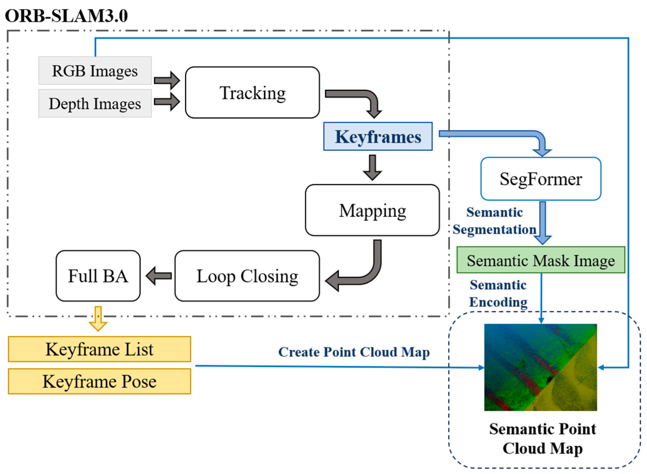
ORB-SLAM [31] is a vision-based simultaneous localization and mapping (SLAM) system that matches feature points extracted from correlated RGB frames through image processing. It selects key frames that comprehensively cover the camera’s spatial trajectory to achieve real-time pose estimation within its operational space. ORB-SLAM 3.0 [32] employs a multi-feature map approach for large-scale scene representation, enhancing both the positioning accuracy of visual SLAM and providing stable pose estimation support for facility-based greenhouse scene reconstruction. However, this algorithm exhibits limited performance in low-texture greenhouse environments and lacks the capability to construct high-density point cloud maps of scenes. Incorporating semantic information can enhance its ability to represent facility-based greenhouse scenes.

Enhancing the representation of greenhouse environments through semantic information and reconstructing dense point clouds of the scene, the introduction of semantic segmentation and point cloud map reconstruction threads in ORB-SLAM 3.0 forms the semantic reconstruction SLAM algorithm, whose structure is shown in Figure 6. The semantic segmentation thread is based on the Segformer-B0 network, capable of running in parallel with the original framework to obtain semantic mask maps at the same resolution as the camera images. The semantic mask map at the same resolution is input alongside the original image into the point cloud map reconstruction thread. Utilizing the camera pose information solved by the SLAM algorithm and the depth information acquired by the depth camera, the color point cloud map and the semantic point cloud map of the scene are reconstructed.

Figure 6. Structure diagram of SLAM semantic point cloud map reconstruction algorithm.

The ORB-SLAM 3.0 algorithm comprises three concurrently running threads. The tracking thread processes the RGB image and depth map input for each frame, extracting feature points through image processing and matching them against the current local feature map to estimate the camera pose $T_f\in SE\left(3\right)$ in real time for each frame. The core of the pose estimation process involves minimizing the reprojection error of feature points, as shown in Equation (6). Here, $X_i$ represents the map point in world coordinates, $x_i$ denotes its corresponding image pixel coordinate, $\phi$ is the projection function of the depth camera, and ${\rho }_H$ is the Huber robust kernel function, which reduces the impact of outliers and noise on the optimization problem. ${\parallel ·\parallel }_{\sum }^2$ is the weighted L2 norm, where the weights are determined by the covariance matrix $\mathsf{\Sigma }$ defined by the camera’s intrinsic parameters. The use of a depth camera provides initial estimates for $X_i$ through depth information. This depth information is then applied via the projection function $\phi$, enhancing the stability and reliability of the pose estimation.

$$T_f^{*}=arg\underset{T_f}{min}\sum _i{\rho }_H\left({\parallel x_i-\phi (T_f\cdot X_i)\parallel }_{\mathsf{\Sigma }}^2\right)$$

(6)

The local mapping thread is responsible for maintaining and optimizing the local map. It inserts keyframe feature points selected by the tracking thread into the feature map and performs bundle adjustment between local keyframes and map points using co-view relationships, ensuring the accuracy and consistency of the local feature map. The loop closure detection thread identifies whether the camera has returned to previously visited areas. Upon detecting a loop closure through feature matching, the algorithm performs global pose optimization to correct cumulative offsets. The ORB-SLAM 3.0 algorithm acquires the keyframe list KFs required for point cloud reconstruction along with their corresponding poses $\{T_{K{F}_1},T_{K{F}_2},T_{K{F}_3},\dots \}$. Keyframes are not selected frame-by-frame; instead, the algorithm judges the richness of scene changes based on the number of matched scene features and selects them at intervals of several frames. This strategy balances computational efficiency during reconstruction with the completeness of reconstructed map information.

After implementing trajectory tracking, the camera transformation matrix $T_f\in SE\left(3\right)$ can be obtained. The RGB-D camera captures the scene’s color image $C_f$ and its corresponding depth image $D_f$. Let $K_c$ denote the internal parameter matrix of the RGB camera, and $R_d\in SE\left(3\right)$ denote the external parameter matrix between the depth camera and the RGB camera. Since the RGB image and the semantic feature map $S_f$ share the same height and width and maintain identical projection relationships within the scene, the spatial point representation of any pixel $(u,v)$ in the image can be calculated using Equation (7). By iterating over the entire keyframe set KFs and computing the local point cloud map for each keyframe, the fusion of local point clouds from different keyframes enables the construction of both the scene point cloud map and the semantic point cloud map, as shown in Equation (8). Here, ${\Omega }_f$ denotes the set of pixels with valid depth values. The final semantic point cloud requires the removal of sparse noise points within a certain range whose neighborhood point count is less than $\rho$.

$$Poin{t}_{\left(x,y,f\right)}=\left\{T_f^{-1}\cdot R_d\cdot \left[D_f\right(u,v)\cdot K_c^{-1}[u,v,1{]}^T{]}^T,C_f(u,v),S_f(u,v)\right\}$$

(7)

$$MP=\bigcup _{f\in KFs}Poin{t}_{\left(x,y,f\right)}\left|\right(x,y)\in {\Omega }_f$$

(8)

Algorithm 1: Visual SLAM Point Cloud Reconstruction Algorithm Incorporating Segformer

Input: Images captured from the camera with timestamps: ($C_f$, $D_f$, timeStamp) SegformerNet: Trained semantic segmentation network Intrinsic Parameters: $K_c$, Extrinsic Parameters: $R_d$, Noise Filtering Threshold: $\rho$

Output: Global Semantic Point Cloud: MP

Global variables: KFs <- {}  //Keyframe Set MP <- {}  //Global Semantic Point Cloud DataBuffer <- ThreadSafeQueue ()  //Thread-safe Queue for Synchronizing Data

1:  System::Run ()  //Main Program 2:  ORB_SLAM3.Initialize () 3:  Segformer.LoadModel () 4:  launch_thread (ORB_SLAM3_Track) 5:  launch_thread (SemanticSegmentation_Thread) 6:  launch_thread (PointCloudReconstruction_Thread) 7:  wait_for_all_threads_to_finish () 8: 9:  Thread1 ORB_SLAM3 () //Visual SLAM Thread 10:    while not terminated do 11:        ($C_f$, $D_f$, timeStamp) <- GrabFrame() 12:        $T_f^{*}$ <- ORB_SLAM3.Track ($C_f$, $D_f$) 13:        if IsNewKeyFrame ($f_i$) then 14:            KFs.add ($f_i$) 15:            SegmentQueue.add ($f_i$) 16:        end if 17:        DataBuffer.push (($C_f$, $D_f$, $T_f$, timeStamp)) 18:        ORB_SLAM3.Mapping () 19:        $T_f$ <- ORB_SLAM3.LoopClosing ($T_f^{*}$) 20:        KFs. $f_i$. $T_f$ <- $T_f$ 21:        end while 22: 23:   Thread2 SemanticSegmentation () //Semantic Segmentation Thread 24:       while not terminated do 25:           ($C_f$, timestamp) <- SegmentQueue.pop ($f_i$) 26:           $S_f$ <- SegformerNet.predict ($C_f$) 27:           DataBuffer.update (($S_f$, timeStamp)) 28:       end while 29: 30:     Thread3 SemanticReconsturctionThread (): //Semantic Reconstruction Thread 31:         while not terminated do 32:             if NewKeyFrameAvailable () then 33:                 ($C_f$, $D_f$, $T_f$, $S_f$) <- KeyframeQueue.pop () 34:                 LocalPointCloud <- {} 35:                 for each pixel $(u,v)$ in $C_f$ do 36:                     if $D_{f }(u,v)$ > 0 then 37:                        $Poin{t}_d$ <- $D_f(u,v)$ * $K_c^{-1}$ * $[u,v,1{]}^T$ 38:                        $Poin{t}_{word}$ <- $T_f^{-1}$ * [$R_d$ * $Poin{t}_d$; 1] 39:                        LocalPointCloud.add ($Poin{t}_{word}$.x, $Poin{t}_{word}$.y, $Poin{t}_{word}$.z, $C_f(u,v)$, $S_f(u,v)$) 40:                     end if 41:                 end for 42:                 MP.add (LocalPointCloud) 43:                 MP <- RemoveOutliers (MP, $\rho$) 44:              end if 45:          end while

To achieve path planning for robotic operations, the reconstructed semantic point cloud map must first be converted into a two-dimensional semantic raster map. Each point in the semantic point cloud can be represented as $MP=\left\{\right(x_i,y_i.z_i,S_{fi}\left)\right|i=\mathrm{1,2},\dots ,n\}$, where $S_{fi}$ denotes the category feature vector for each point. Since the scene point cloud is primarily distributed near planting surfaces and paved roads, the ground surface traversed by the robot can be considered the dominant plane for reconstructing the point cloud. The Randomized Agreement of Samples by Consistency (RANSAC) method [33] is employed to extract the dominant plane of the reconstructed point cloud: $\mathsf{\Pi }:n^{T}x+b=0$. The core process of this algorithm involves generating candidate plane models through iterative random sampling of point sets. The internal point set of each plane is determined based on the distances of points within the point cloud to the candidate planes. Finally, the optimal plane model is selected as the dominant plane of the point cloud by maximizing the size of its internal point set. Rigid transformations $T_M\in SE\left(3\right)$ can rotate the point cloud from the sampling coordinate system to the ground coordinate system, as shown in Equations (9) and (10).

$$R_M\cdot n=[0,0,1{]}^T,{ t}_M={\left[0,0,b\right]}^T, T_M=\left[\begin{array}{cc}{R}_M& t_M\\ 0& 1\end{array}\right]$$

(9)

$${[x}_i,y_i,z_i,1{]}^T\cdot T_M=\left[x_i^{\prime },y_i^{\prime },z_i^{\prime },1\right]$$

(10)

The process of constructing a semantic grid map is described by Equations (11) and (12). In the ground coordinate system, using the ground as the projection plane, the point cloud can be divided into two-dimensional square grids $G_{m,n}$ with side length $d_0$. This yields a set of candidate points $P_{m,n}$ within each grid $G_{m,n}$ whose heights fall within the range $[-h_0,h_0]$, as shown in Equation (6).

$$P_{m,n}=\left\{\left(x_i^{\prime },y_i^{\prime },z_i^{\prime },S_{fi}\right)\in MP|\left(x_i^{\prime },y_i^{\prime }\right)\in G_{m,n},-h<z_i^{\prime }<h\right\}$$

(11)

The grid category is determined by the semantics of all points it contains, as shown in Equation (12), where $N_{P_{m,n}}$ denotes the number of points in the point set $P_{m,n}$. $Linea{r}_{class}(C\to N_{class})$ denotes the linear classifier (dim = [$N_{class}, C, 1, 1$]), which calculates the corresponding grid category $S_{m,n}$ using the computed feature vectors from each grid. Since the feature vectors of points in the point cloud perfectly correspond to those in the Segformer fusion feature map, we directly adopt the linear classifier from the Segformer decoder head while preserving the same weights and bias terms without additional training. This approach avoids the need for point-by-point statistical analysis of semantic category proportions within each grid cell during semantic map conversion. It reduces the computational time required for large-scale point cloud conversion, thereby significantly improving the efficiency of map conversion.

$$S_{m,n}(dim=N_{class})=Linea{r}_{class}(C\to N_{class})[{\displaystyle \frac{1}{N_{P_{m,n}}}}\sum _{\left(x_i^{\prime },y_i^{\prime },z_i^{\prime }\right)\in P_{m,n}}{S}_{fi}(dim=C)]$$

(12)

2.2.4. SC-A* Path Planning Algorithm Based on Scene Semantic Constraints

The path generation problem for weed-removing robots in greenhouse facilities can be summarized as a path planning problem constrained by target points and obstacles. Its essence lies in finding the shortest path from the initial state to the target state within the navigable space defined by grid map semantics and robot motion characteristics.

In the scenario of generating operational paths within greenhouses, the system must simultaneously address multi-obstacle environmental constraints formed by boundaries, crops, and operational equipment, while meeting core requirements for path generation efficiency and global optimality. For such constraints and requirements, the A* algorithm [34] demonstrates adaptability advantages by incorporating heuristic guidance to enhance search efficiency while ensuring globally optimal path outputs. This algorithm quantifies the comprehensive cost of each state $s_k=(x_k,y_k,{\theta }_k)$ through the heuristic cost function $f\left(s_k\right)$, as expressed in Equation (13). This cost is jointly determined by the cumulative cost $g\left(s_k\right)$ and the heuristic cost $h\left(s_k\right)$, where the heuristic cost estimate $h\left(s_k\right)$ is based on the Euclidean straight-line distance from state $s_k$ to the target state $s_f$, enabling heuristic guidance of the search direction.

$$\begin{gathered} f\left(s_k\right)=g\left(s_k\right)+h\left(s_k\right) \\ g\left(s_k\right)=\sum _{i=1}^{k}cost\left(s_{i-1},a_i\right) \\ h(s_k)=\sqrt{(x_k-x_f{)}^2+(y_k-y_f{)}^2} \end{gathered}$$

(13)

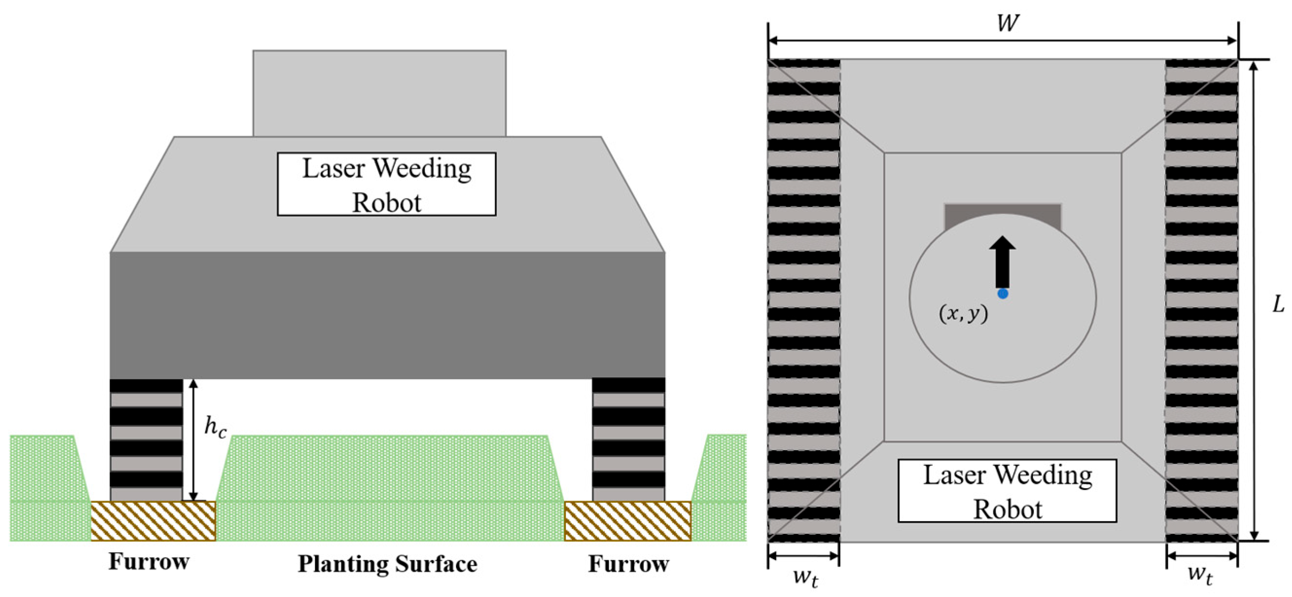
To describe the motion characteristics of the weeding robot, its two-dimensional model is abstracted as a rectangular structure (as shown in Figure 7): with length L and width W, featuring two tracks of length L and width $w_t$ on either side. The body section between the tracks does not contact the ground. When operating in greenhouse cultivation areas, both tracks traverse the furrows while the chassis remains elevated above the planting surface. Steering is achieved through a dual-track differential drive for on-the-spot turning, enabling adaptation to narrow working spaces.

Figure 7. Laser weeding robot operational mode diagram (left) and dimensions diagram (right).

To enable the robot to perform coordinate transformations between its local and global coordinate systems, given the current state $s=(x,y,\theta )$, the local coordinates $(x_l,y_l)$ of any point on its body can be mapped to global coordinates $(x_g,y_g)$ using Equation (14). This provides the foundation for subsequent spatial occupancy and constraint detection.

$$\left[\begin{array}{c}{x}_g\\ y_g\end{array}\right]=\left[\begin{array}{cc}cos\theta & -sin\theta \\ sin\theta & cos\theta \end{array}\right]\left[\begin{array}{c}{x}_l\\ y_l\end{array}\right]+\left[\begin{array}{c}{x}_c\\ y_c\end{array}\right]$$

(14)

Based on the actual operational requirements of weeding tasks, the robot must satisfy terrain semantic constraints: the tracks may traverse furrows (S₁) and paved surfaces (S₃), but must not contact the planting surface (S₂) to prevent crop damage; the central body may cross the planting surface (S₂), and the entire machine must completely avoid other obstacles (S₀). To quantify these constraints, define the grid space occupied by the vehicle body in the current state as $C_{ve}\left(s\right)$ (as shown in Equation (15)), and the space occupied by the tracks as $C_{trac}\left(s\right)$ (as shown in Equation (16)). Based on this, the terrain semantic constraint $\mathsf{\Theta }\left(s\right)$ at any state can be expressed as in Equation (17), where $S(x,y)$ denotes the semantic attribute of grid point $(x,y)$.

$$C_{ve}\left(s\right)=\left\{\left(x_g,y_g\right)|x_l\in \left[-{\displaystyle \frac{L}{2}},{\displaystyle \frac{L}{2}}\right],y_l\in \left[-{\displaystyle \frac{W}{2}},{\displaystyle \frac{W}{2}}\right]\right\}$$

(15)

$$C_{trac}\left(s\right)=\left\{\left(x_g,y_g\right)|x_l\in \left[-{\displaystyle \frac{L}{2}},{\displaystyle \frac{L}{2}}\right],y_l\in \left[-{\displaystyle \frac{W}{2}},-{\displaystyle \frac{W}{2}}+w_t\right]\cup \left[{\displaystyle \frac{W}{2}}-w_t,{\displaystyle \frac{W}{2}}\right]\right\}$$

(16)

$$\mathsf{\Theta }\left(s\right)=\left\{\begin{array}{c} \forall \left(x_i,y_i\right)\in C_{ve}\left(x_i,y_i\right) :S\left(x_i,y_i\right)=S_1, S_2 or S_3\\ \forall \left(x_i,y_i\right)\in C_{trac}\left(x_i,y_i\right) :S\left(x_i,y_i\right)=S_1 or S_3\end{array}\right.$$

(17)

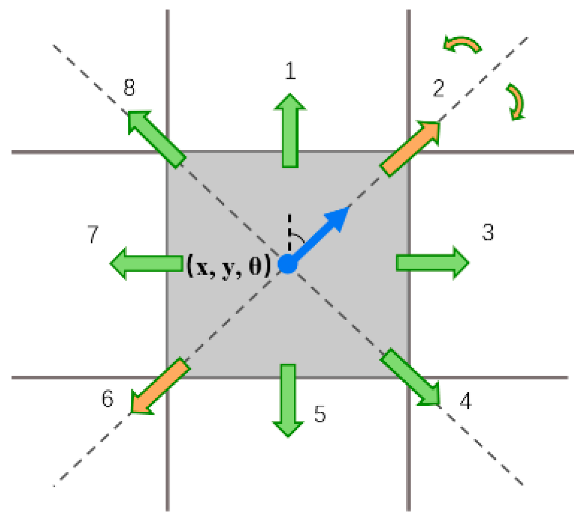
The traditional A* algorithm supports an action space with 8 displacement directions and 2 turning directions per step. However, due to kinematic constraints on this tracked robot, each orientation change necessitates recalculating semantic constraints under the new state, significantly increasing computational complexity. To simplify constraint verification during turning, this paper specifically optimizes the trajectory search range. Only translation movements aligned with the robot’s current orientation (forward and backward) are retained. Each step considers only clockwise and counterclockwise 45° turning angles, as shown in Figure 8, where the orange arrows indicate the optimized search range.

Figure 8. Schematic diagram of the SC-A* algorithm search space. Orange arrows indicate the range.

Based on the above descriptions of the cost function, semantic constraints, and action space, the task path generation problem within the greenhouse can be abstracted as follows: within the discrete state space $S_c$, find an action sequence $A=(a_1,a_2,\dots ,a_n)$ from the initial state $s_0$ to the target state $s_f$ that satisfies Equation (18), where $T(s_{k-1},a_k)$ denotes the state transition function from state $s_{k-1}$ to state $s_k$, determined by action $a_k$ from the action space A₀, and each state $s_k$ satisfies the constraint $\mathsf{\Theta }\left(s\right)$.

$$P=\underset{A}{min}\sum _{k=1}^{n}cost\left(s_{k-1},a_k\right) , { s}_k=T\left(s_{k-1},a_k\right) and \mathsf{\Theta }\left(s_k\right)$$

(18)

Algorithm 2: SC-A* Algorithm

Input: Grid map: G Initial state: $s_0=(x_0,y_0,{\theta }_0)$ Target State: $s_n=(x_n,y_n,{\theta }_n)$ Robot Length: L, Robot Width: W, Track Width: $w_t$

Output: Path: State sequence from the starting point to the target point

Global variables: PendingState: Priority queue, storing the current states to be searched, sorted in ascending order by $f\left(s_k\right)$. VisitedState: Set, store evaluated states gScore: Dictionary, storing the minimum known cost from the starting point to each state lastState: Dictionary, storing the predecessor state for each state, used for path reconstruction

1:  Function SC_A_Star (G, $s_0$, $s_n$, L, W, $w_t$): 2:      PendingState.add ($s_0$) 3:      gScore($s_0$) <- 0 4:      fScore($s_0$) <- EuclideanDistance ($s_0$, $s_n$) //the predicted shortest path (Euclidean distance) 5: 6:      while PendingState is not empty do 7:          $s_k$ <- PendingState.pop_min_fScore () //prioritize updating states that minimize the loss function. 8:          if $s_k$ is $s_n$ then 9:              return ReconstructPath (lastState($s_k$), $s_k$) 10: 11:          VisitedState.add ($s_k$) 12:          for each $a_i$ in PossibleAction ($s_k$) do 13:              nextState <- ApplyAction ($s_k$, $a_i$) 14:              if nextState in VisitedState then 15:                  continue 16:              end if 17:              if not ValidSemanticConstraints (nextState, G) then //check whether semantic constraints are satisfied 18:                  continue 19:              end if 20:              tentative_gScore <- gScore($s_k$) + Cost ($s_k$, nextState) 21:              if nextState not in PendingState or tentative_gScore < gScore (nextState) then 22:                  lastState (nextState) <- $s_k$23:                  gScore (nextState) <- tentative_gScore 24:                  fScore (nextState) <- gScore (nextState) + EuclideanDistance (nextState, $s_n$) 25:                  if naxtState not in PendingState then 26:                      PendingState.add (nextState) 27:                  end if 28:              end if 29:          end for 30:      end while 31: 32:      return NULL //No valid path found 33: 34:  Function ValidSemanticConstraints (State, G): 35:       $C_{ve}$, $C_{trac}$ <- CalculateOccupiedGrids (State, G, W, L, $w_t$) 36:       for each grid in $C_{trac}$ do //verify track restraint 37:          $S_{grid}$ <- G.getSemantic (grid) 38:          if $S_{grid}$ is not $S_1$ and $S_{grid}$ is not $S_3$ then 39:             return false 40:          end if 41:       end for 42:       for each grid in $C_{ve}$ do //verify vehicle restraint 43:          $S_{grid}$ <- G.getSemantic (grid) 44:          if $S_{grid}$ is $S_0$ then 45:             return false 46:          end if 47:       end for 48: 49:       return true

3. Results

3.1. Semantic Segmentation Performance Evaluation

The semantic segmentation performance evaluation aims to validate the accuracy and real-time capability of the adopted lightweight semantic segmentation network in multi-span greenhouse environments. This experiment was conducted on a workstation equipped with an NVIDIA RTX 4090 GPU running the Ubuntu 20.04 operating system. The preparation and partitioning process of the experimental dataset is shown in Section 2.1.3. The evaluation employs metrics commonly used for semantic segmentation: Intersection over Union (IoU), Accuracy (Acc), F1-score, and Overall Accuracy (OA).

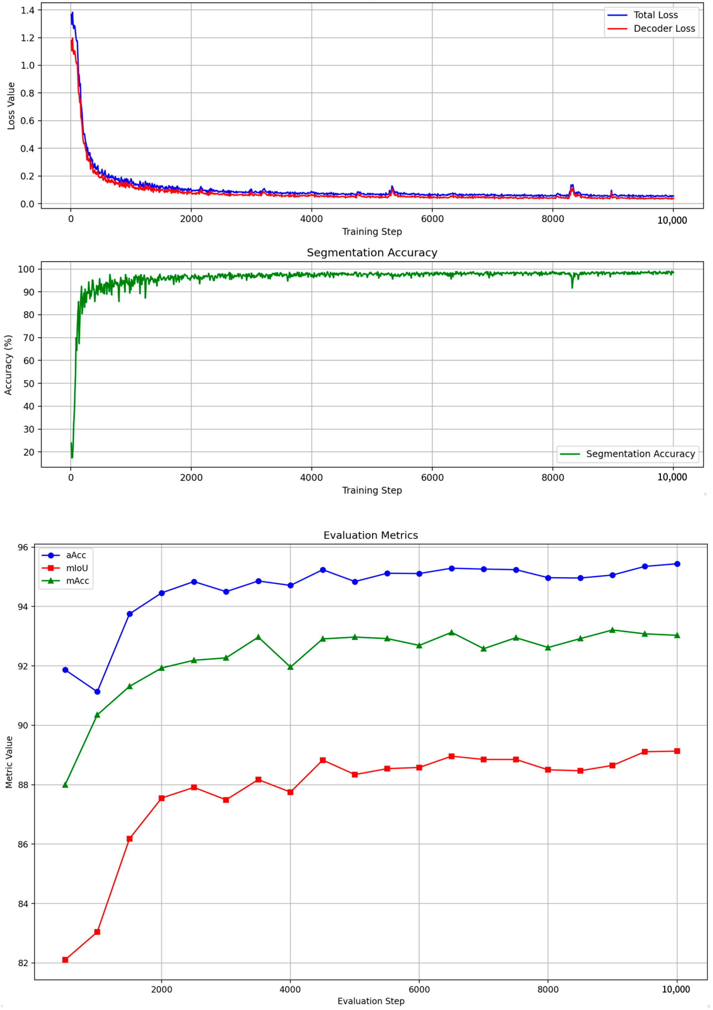
For model training, our Segformer-B0 model employs the AdamW optimizer with momentum set to [0.9, 0.999] and weight decay of 0.01. The initial learning rate is 6 × 10⁻⁵, with linear scheduling for warm-up during the first 1500 epochs, followed by Poly scheduling for learning rate decay. Input images were resized uniformly to 640 × 480 pixels. With a batch size of 8, the model underwent 10,000 training epochs. The model achieving optimal performance on the validation set was selected for evaluation. Figure 9 illustrates the variation curves of the loss function and accuracy on the training set, along with the evaluation metrics on the validation set, as training iterations increase during the model training process. As seen in the figure, metrics on the training set gradually flatten and converge during training, while evaluation metrics on the validation set increase and stabilize over training, indicating no underfitting. Furthermore, accuracy on both the validation and training sets remains essentially identical and stable, showing no significant overfitting.

Figure 9. Curves showing changes in the loss function on the training set (top), accuracy on the validation set (middle), and evaluation metrics on the test set (bottom) as training progresses.

Through grid search, we determined the network weights α = 0.7 on the validation set. This configuration fully leverages the advantages of weighted cross-entropy loss and Dice loss for segmentation. The weights for each category in the weighted cross-entropy loss function are calculated based on the inverse frequency of each category’s pixels in the training set. The comparative evaluation results of different loss functions are presented in Table 1. Table 2 displays segmentation results achieved by the Segformer network on our proprietary dataset, achieving an mIoU of 89% across all categories with an overall accuracy exceeding 95%. The network achieves its highest segmentation accuracy on paved surfaces, exceeding 99%. Segmentation precision in ridge areas is slightly lower than in cultivated land surfaces, reaching 83%. Compared to using the cross-entropy loss function alone, segmentation accuracy for the ridge category improves by 3.9%. Compared to using the Dice loss function alone, the hybrid loss function increases overall accuracy (OA) by 2.3%.

Table 1. Results of the Segformer algorithm in the test set.

Class	IoU/%	Acc/%	F1-Score	mIoU/%	OA/%
Background	81.43	83.88	89.8	89.13	95.44
Furrow	83.21	92.90	90.84
Planting Surface	93.43	96.78	96.6
Paved road	98.41	99.31	99.2

Table 2. Comparison of Segmentation Results Metrics Across Different Loss Functions.

Model	mIoU/%	OA/%	mF1-Score	Furrow IoU/%
only wce loss	88.56	94.31	92.84	79.37
only Dice loss	86.31	93.13	91.03	80.07
wce loss + Dice loss	89.13	95.44	93.40	83.21

To evaluate our network’s performance on this task, its results were compared against lightweight convolutional semantic segmentation networks PSP-Net and DeepLabV3+, as well as the Transformer-based semantic segmentation network Swin-Tiny. Additionally, segmentation results from the loss-tuned network (adj) were contrasted with those from the original network (ori). Hyperparameters for each network were tuned using grid search, with the following parameters explored: (1) Optimizers: AdamW and SDG, (2) Initial learning rate: [5 × 10⁻⁴, 1 × 10⁻⁴, 5 × 10⁻⁵, 1 × 10⁻⁵], (3) Weight decay: [0.1, 0.05, 0.01]. The optimized hyperparameter settings for each model are shown in Table 3. The training batch size was set to 8. Training was terminated after 50 epochs when no significant improvement in validation performance was observed, thereby preventing overfitting or underfitting.

Table 3. Hyperparameters for Comparison Models.

Model	BackBone	Optimizer	Learning Rate	Weight Decay
PSP-Net	ResNet-50	AdamW	1 × 10−4	0.01
DeepLabV3+	ResNet-50	SGD	1 × 10−4	0.01
Swin + upperNet	Swin-Tiny	AdamW	5 × 10−5	0.01
Segformer-B0	MiT-B0	AdamW	6 × 10−5	0.01

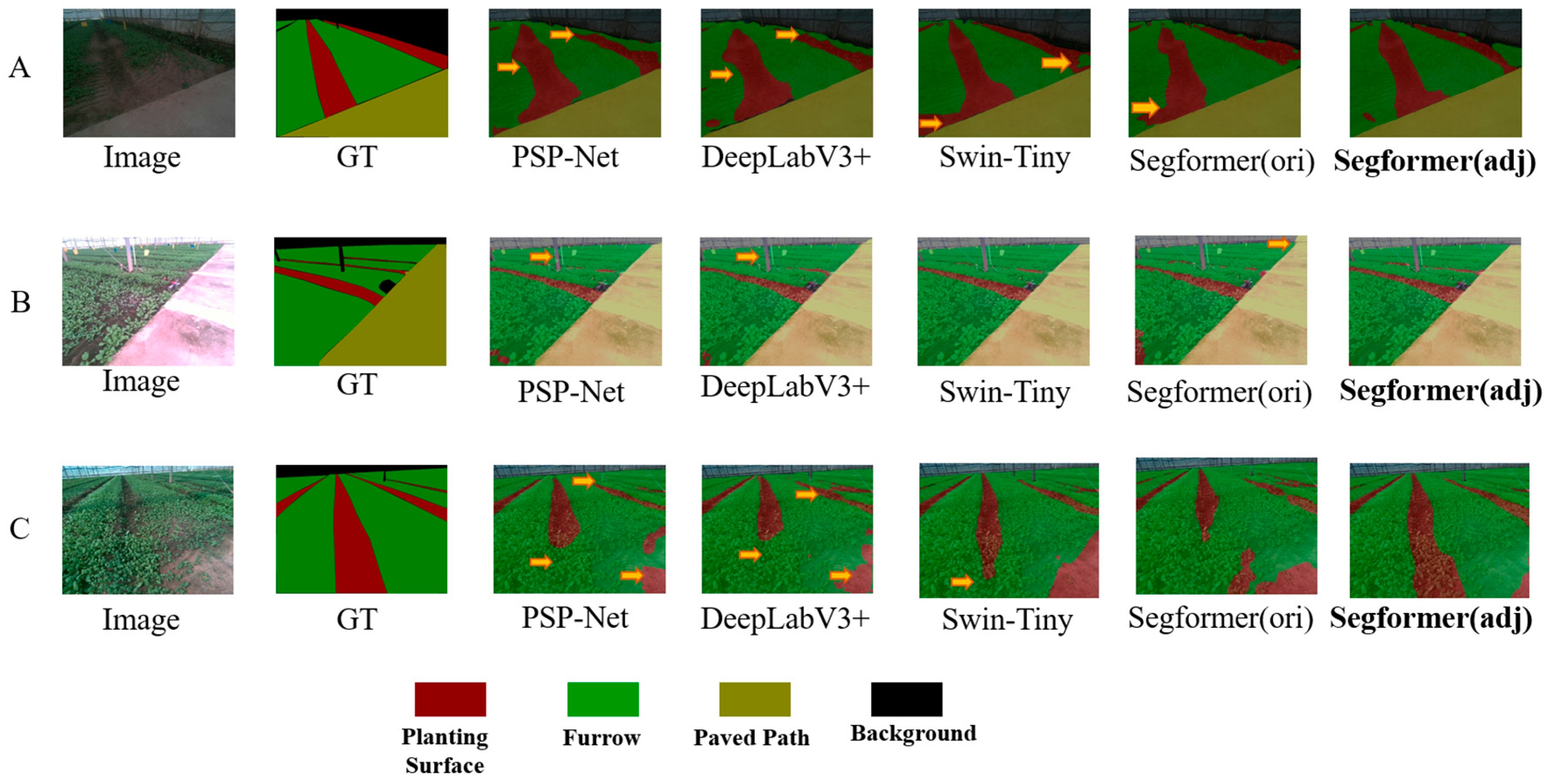
Figure 9 displays segmentation results for vegetable field scenes across different environmental conditions. For vegetables growing within furrows (Figure 10A), the Transformer-based segmentation network demonstrated superior performance in learning global features of furrow shapes. In scenes with color distortion due to camera overexposure (Figure 10B), the convolutional-based semantic segmentation network exhibited significant errors in identifying slender objects like steel support poles, while the Segformer network maintained robust performance. Under overcast conditions with dim lighting (Figure 10C), all networks exhibited segmentation errors at the boundaries where planting surfaces and furrows were covered by green vegetation. However, the fine-tuned SegFormer network could still recognize the basic shape features of furrows. Compared to the original network, the fine-tuned SegFormer network demonstrated improved resolution at certain boundary locations between different categories and better discrimination of crop encroachment into furrows.

Figure 10. Comparison of Segformer with other semantic segmentation algorithms in greenhouse scenarios. (A) Overcast conditions with low light. (B) Direct sunlight causing camera overexposure. (C) Vague edges due to cabbage scattered in furrows. Orange arrows highlight differences in segmentation details across networks.

Table 4 lists the evaluation metrics for each network and compares their parameter counts and frame rates during inference tasks. To assess accuracy in minor road semantic segmentation, the Intersection over Union (IoU) metric for ditches was added to all networks. As shown in Table 4, the SegFormer network performs comparably to the other three comparison networks on comprehensive image semantic segmentation metrics while demonstrating improved segmentation results for the ditch category. Furthermore, the SegFormer network employs significantly fewer parameters than comparable segmentation networks, enabling it to achieve notably higher frame rates during semantic segmentation tasks. The fine-tuned network demonstrates superior boundary discrimination for ditches compared to the original model, resulting in enhanced overall segmentation accuracy.

Table 4. Performance comparison of different semantic segmentation algorithms on the test set.

Model	mIoU/%	OA/%	mF1-Score	Furrow IoU/%	Fps	Parameters
PSP-Net	87.11	94.34	92.9	79.73	101.83	46.603 M
DeepLab V3+	87.31	94.48	93.03	80.07	63.76	41.217 M
swin-tiny	88.8	95.17	93.92	81.94	44.12	120 M
Segformer (ori)	86.58	94.12	92.87	78.15	120.33	3.716 M
Segformer (adj)	87.93	94.7	93.4	83.21	121.56	3.716 M

3.2. Evaluation of Semantic Map Reconstruction Results

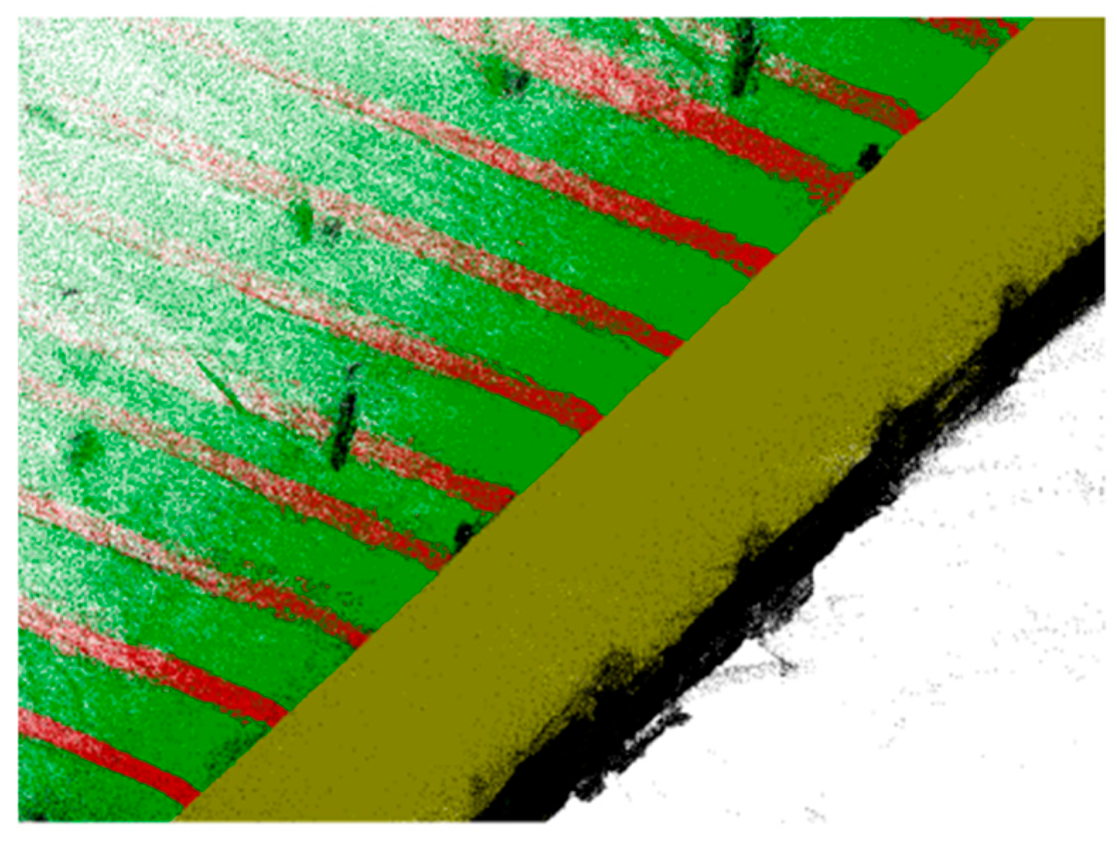
The reconstruction results of the semantic map reconstruction algorithm are shown in Figure 11. Three-dimensional reconstruction typically evaluates the accuracy of reconstructed point clouds using metrics such as Euclidean distance, Chamfer Distance (CD), and structural similarity index between the reconstructed point cloud and the true model. Since obtaining the true model of the agricultural greenhouse environment is challenging, four easily measurable features—paved surface width, steel support pole spacing, planting surface width, and furrow width—were selected as reconstruction error metrics to evaluate semantic map reconstruction accuracy. Paved surface width measurements were calibrated using steel support poles as reference points. Support pole spacing was calculated as the average of measurements taken at heights of 10 cm, 20 cm, and 30 cm above ground level. Planting bed width and furrow width were calculated as the average of measurements taken at distances of 1 m, 3 m, and 5 m from the paved surface. The average relative error (MRE) and average absolute error (MAE) for the reconstruction results of these four feature types are shown in Table 5.

Figure 11. Dense semantic point cloud of facility greenhouse scenes.

Table 5. Reconstruction results of semantic reconstruction algorithms across various categories.

Class	Reconstructed Mean/m	Measurement Mean/m	MAE/cm	MRE/%
support pole spacing	7.99	8.00	11	1.43%
paved road width	2.07	2.09	4	1.88%
planting surface width	1.31	1.27	7	5.28%
furrow width	0.40	0.42	3	7.37%

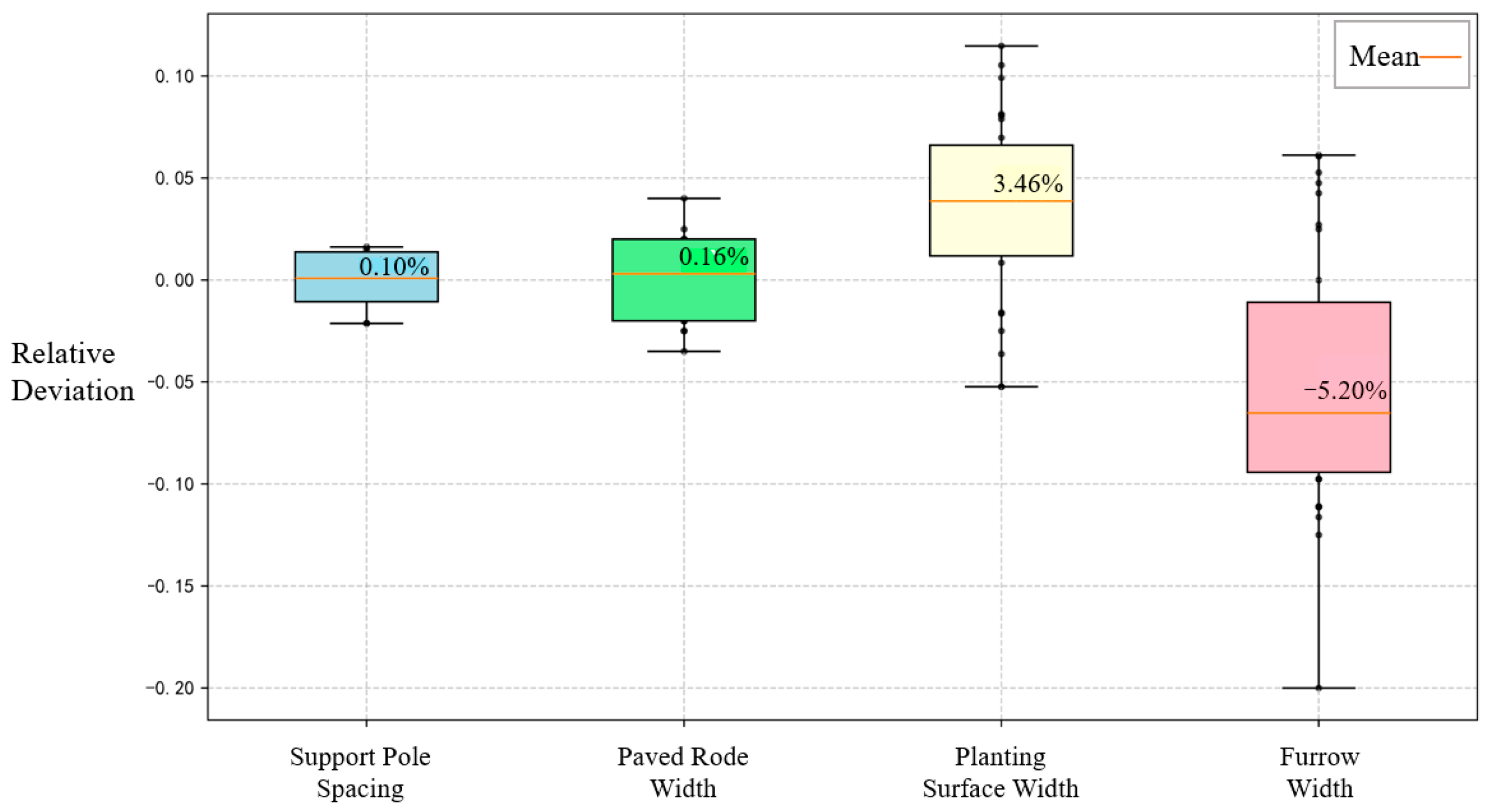
As shown in Table 5, the reconstructed point cloud map exhibits reconstruction errors of <2% for both support pole spacing and paved road width, indicating that the point cloud map reconstructed via the depth SLAM algorithm preserves relatively accurate scene dimensional information. Measurements of the 3D semantic point cloud map yielded average relative reconstruction errors of 5.28% for the planting surface and 7.37% for the furrow width, with the lowest reconstruction accuracy observed for the furrows. Figure 12 shows the distribution of relative deviations between measured values and true values across different categories.

Figure 12. Distribution map of relative size deviations among different categories in the reconstructed point cloud.

3.3. Path Planning Experiment Evaluation

By capturing semantic point cloud maps of the greenhouse, the experiment utilized point-by-point semantic statistics within a small area to generate simulated semantic raster maps, enabling path planning algorithm experiments for weeding robots. The simulation tracked the robot’s transition from an active planting bed to a designated position on an adjacent, unprocessed bed. To ensure all algorithms generated reasonable path plans, semantic constraints were applied to the comparison algorithms based on the dimensions of the vehicle’s elevated chassis. This ensured the robot remained above both the planting bed and the paved surface, simulating the typical operational scenario where the vehicle’s chassis is elevated between two furrows during actual fieldwork.

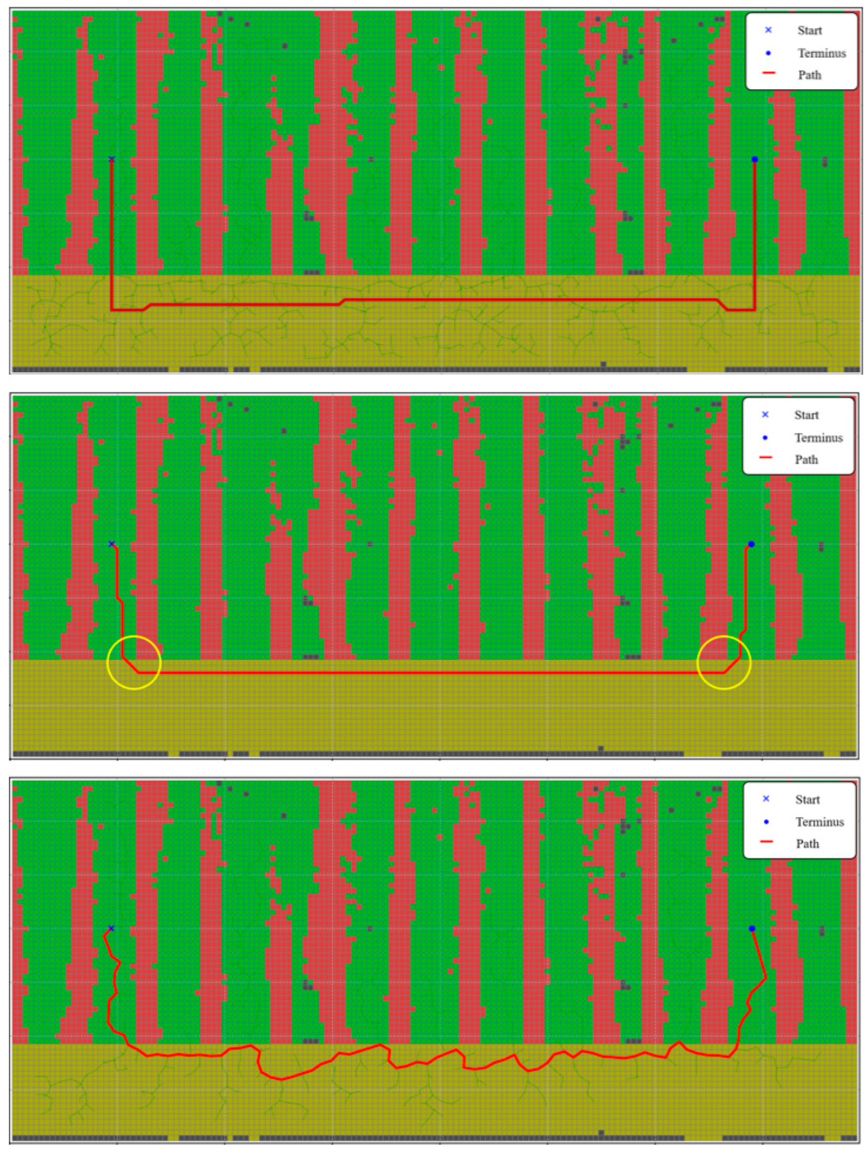
Figure 13 shows the robot planning routes generated by the traditional A* algorithm, RRT algorithm, and SC-A* algorithm. The traditional A* algorithm, due to insufficient semantic constraints, experiences semantic interference at the junction between planted surfaces and paved roads, marked by yellow circles in the figure. The SC-A* algorithm employs a detour strategy, planning space for the robot’s tracks to turn in place.

Figure 13. RRT algorithm (top), A* algorithm (middle), and SC-A* algorithm (bottom) comparisons in a simulated environment.

The number of violations (overriding planted objects or colliding with walls) for paths planned by each algorithm was counted. Metrics such as computation time, path length, and number of turns were compared across algorithms. Table 6 shows that the SC-A* algorithm’s prediction time is slightly shorter than the traditional A* algorithm, while the RRT algorithm takes longer and requires more turns. This indicates that heuristic search enhances path planning efficiency by providing the direction toward the search target. All three algorithms successfully completed the path planning task. The SC-A* algorithm did not encounter any semantic interference, whereas the other two algorithms both experienced semantic interference phenomena.

Table 6. Comparison of simulation results for each algorithm.

Algorithm	Path Length	Computation Time	Violations Times	Turning Times
Traditional A*	161.142	0.134 s	4	9
RRT	184.978	0.378 s	11	62
SC-A*	172.433	0.124 s	0	8

3.4. Algorithm Experiment Evaluation in Real-World Environments

To validate the feasibility and robustness of the proposed real-time semantic reconstruction and weeding path planning algorithm framework for facility greenhouses under actual operating conditions, experiments were conducted to test the algorithm’s operation on a vehicle-mounted computing platform across three greenhouse environments during different growth stages of Chinese cabbage. The sampling vehicle first autonomously traversed paved surfaces to collect data, then utilized the onboard computing unit to perform scene reconstruction and operational path generation calculations for the respective greenhouse environment.

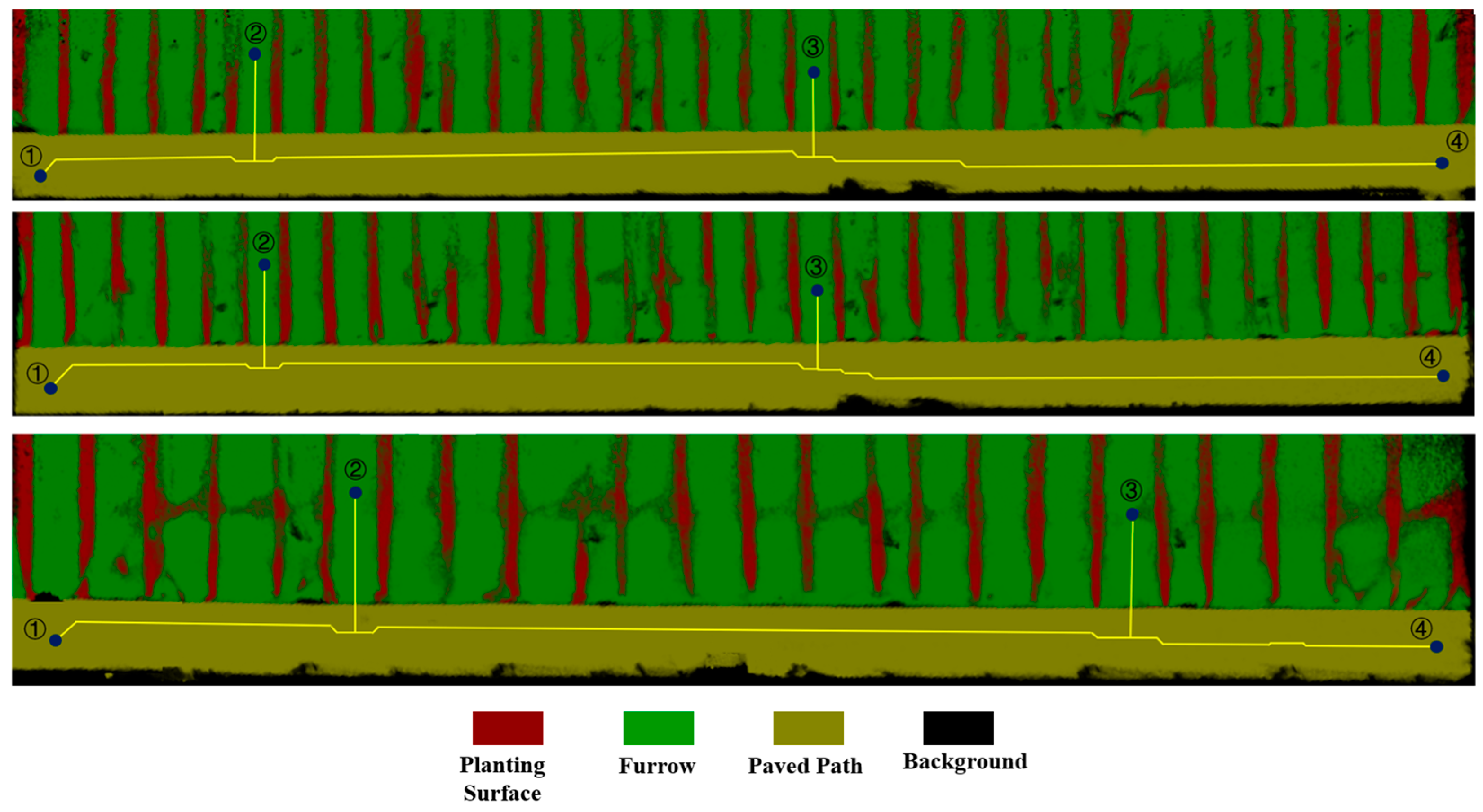
Figure 14 displays the environmental conditions of three facility agriculture greenhouses used in the system experiments. Greenhouse 1 houses mature Chinese cabbage plants with dense growth, obscuring the boundary between the planting surface and furrow edges; Greenhouse 2 houses young Chinese cabbage seedlings with short emergence periods, revealing extensive bare soil in the planting area; Greenhouse 3 contains young seedlings after rainfall, featuring moist ground with standing water and moss growth in the furrows. Furthermore, Greenhouse 3 had never been included in the training of the previous semantic segmentation model. The three greenhouses shared similar layouts, with Greenhouse 3 measuring 40 m wide and Greenhouses 1 and 2 approximately 56 m wide. The vehicle-mounted platform simulated a weeding robot performing identical three-step tasks across all three greenhouses: starting from the entrance, operating on the 5th and 15th ridges, and reaching the exit. The experiment evaluated the success rate of semantic scene map reconstruction and task path planning, along with the real-time performance of the algorithms.

Figure 14. Three real greenhouse scenarios for conducting systematic experiments.

When generating semantic raster maps for experimental greenhouses, the grid parameters for the semantic raster map must first be determined. Here, $d_0$ is jointly determined by the design width of our track and the width of the furrows within the greenhouse. The furrow width inside the greenhouse is approximately 30 ± 5 cm, while the laser weeding vehicle’s track is designed to be either 10 cm or 15 cm wide. To balance the accuracy of the raster map with the computational time of the reconstruction process, we set $d_0$ = 5 cm. Given a 15 cm elevation difference between the planting surface and furrows, plus approximately 10 cm height variations relative to paved surfaces, and considering that environmental obstacles typically occupy the height range of 20 cm to 50 cm above ground level, we set $h_0$= 50 cm. This ensures that the generated scene map incorporates valid semantic information for each grid cell while describing the volume of all obstacles.

The average relative error of semantic scene reconstruction results for the three greenhouses is shown in Table 7. The algorithm achieved high-accuracy scene reconstruction across greenhouses with different growth stages of Chinese cabbage and varying environmental conditions. The path planning results for the simulated weeding robot operation are shown in Figure 15. In greenhouses with varying ridge-furrow distributions, the algorithm consistently generates the specified operational path according to task requirements without crushing the planting surface or colliding with obstacles. This fully demonstrates the reliability of semantic scene reconstruction and the feasibility of the path planning algorithm.

Table 7. Semantic Scene Reconstruction Results for Three Greenhouses.

Greenhouse	MRE (Planting Surface)/%	MRE (Furrow)/%
Greenhouse1	5.28%	7.37%
Greenhouse2	7.91%	10.13%
Greenhouse3	6.39%	7.91%

Figure 15. Systematically planned work paths within the three greenhouses. From (top) to (bottom): Greenhouse 1, Greenhouse 2, and Greenhouse 3.

Table 8 evaluates the system’s real-time performance across three scenarios. The point cloud reconstruction time recorded spans from acquiring the semantic mask image to generating a single-frame point cloud and integrating it into the global point cloud map. As shown in Table 5, the system demonstrates excellent real-time semantic reconstruction capabilities for scenes with approximately 1300 keyframes. As scene point cloud memory consumption increases, both semantic segmentation rate and point cloud reconstruction rate decrease in larger-scale scenes. Map conversion for Greenhouses 1 and 2 took approximately 30 s, while Greenhouse 3 required 16 s, indicating that larger map scales cause conversion times to increase sharply. Compared to the method of assigning values to raster cells based on semantic proportion through point-by-point statistics, the latter approach took over 300 s for a single greenhouse map conversion. This demonstrates that using vector-encoded semantic features can significantly enhance map conversion efficiency.

Table 8. Real-time performance evaluation of the system on the in-vehicle computing platform.

No.	Keyframe Number	Semantic Segmentation (s/f)	Point Cloud Fusion (s/f)	Map Conversion (s)	Path Planning (s)
Greenhouse1	1363	0.134	0.339	32.64	0.815
Greenhouse2	1390	0.136	0.355	31.21	0.897
Greenhouse3	898	0.127	0.217	16.45	0.732

4. Discussion

Weed removal, planting, harvesting, and transportation within vegetable greenhouse facilities require robotic navigation systems to achieve precise scene feature description and meet task-oriented automated path generation demands. This paper introduces lightweight real-time semantic segmentation into the visual SLAM algorithm framework for semantic scene reconstruction in greenhouse environments. Based on the transformed map, a task-oriented path planning algorithm for agricultural robots is designed.

(4)

The lightweight semantic segmentation algorithm Segformer achieved a global accuracy of 95.44% and a mIoU of 89.13% on the facility greenhouse dataset. It attained a recognition accuracy of 92.90% for furrows, with the joint loss function yielding a 3.9% improvement over a single loss function. Compared to other algorithms, it features fewer parameters and faster inference speeds.

(5)

The semantic map reconstruction algorithm based on visual SLAM achieves an average relative error of <2% for reconstructing support pole spacing and paved road width within greenhouses, demonstrating high accuracy in scene reconstruction. For the two types of boundaries defined by semantic information—planting surfaces and furrows—the average relative errors in reconstruction were 5.82% and 7.37%, respectively. The average deviation values were 3.46% and −5.20%, indicating high semantic reconstruction accuracy.

(6)

The SC-A* path planning algorithm completed its computation in 0.124 s on the workstation within the experimental simulation scenario. It successfully planned the robot’s operational path, demonstrating higher computational efficiency than the traditional A* algorithm. Additionally, it successfully avoided the planting surface at the junction between the planting zone and paved roadway.

(7)

The system’s feasibility and real-time performance were validated across three greenhouse facilities with distinct environmental conditions. The system successfully reconstructed semantic maps in all three greenhouses and achieved path planning without violating constraints. On the PC in the vehicle platform, semantic segmentation took approximately 0.13 s per frame, point cloud fusion took about 0.35 s per frame, map conversion took roughly 30 s, and path planning completed in under 1 s, meeting real-time requirements.

5. Conclusions

This work demonstrates that by coupling lightweight semantic segmentation networks with visual SLAM systems, semantic information can be integrated into detailed scene representation methods. Maps constructed using this approach can meet the navigation demands of more diverse smart agriculture scenarios. They enable robots to fully leverage their motion characteristics during operations, avoiding crop damage or collisions within the densely planted spaces of greenhouses.

This study proposes a universal real-time semantic point cloud reconstruction and path planning framework, whose semantic module, visual SLAM method, and path planning algorithm can be flexibly switched according to scene requirements. However, the current research still has certain limitations. For example, the pose estimation process of the SLAM system relies solely on feature point reprojection estimates provided by the depth camera, which may result in pose tracking loss in large-scale connected greenhouse scenarios. Future research could integrate semantic information into the pose estimation workflow of the SLAM system, complemented by wheel encoders or inertial sensors, to further enhance the reconstruction accuracy of semantic point clouds. The current path planning algorithm simplifies the motion characteristics of tracked robots without modeling their continuous movement, and lacks adaptability to the kinematic properties of wheeled robots, limiting the solution’s applicability to other scenarios. Future research should incorporate continuous robot kinematic models into the solution process, optimize path search based on movement characteristics and turning radius, and introduce path optimization to achieve smoother trajectories. Furthermore, while the current algorithm primarily targets soil-based greenhouse operations, we aim to enhance the framework’s universality and usability in future work. The framework should become compatible with additional positioning, reconstruction, or path planning modules to strengthen the algorithm’s practicality within precision agriculture applications.

References

1. Lytridis, C.; Pachidis, T. Recent Advances in Agricultural Robots for Automated Weeding. AgriEngineering 2024, 6, 3279–3296. [Google Scholar] [CrossRef]
2. Li, Y.; Guo, Z.; Shuang, F.; Zhang, M.; Li, X. Key Technologies of Machine Vision for Weeding Robots: A Review and Benchmark. Comput. Electron. Agric. 2022, 196, 106880. [Google Scholar] [CrossRef]
3. Autonomous LaserWeeder Demo Unit—Carbon Robotics. Available online: https://carbonrobotics.com/autonomous-weeder (accessed on 6 January 2025).
4. TerraSentia—EarthSense. Available online: https://www.earthsense.co/terrasentia (accessed on 6 January 2025).
5. Ecorobotix: Smart Spraying for Ultra-Localised Treatments. Available online: https://ecorobotix.com/en/ (accessed on 6 January 2025).
6. Our Vision for the Future: Autonomous Weeding (in Development) AVO. Available online: https://ecorobotix.com/en/avo/ (accessed on 6 January 2025).
7. Diao, Z.; Guo, P.; Zhang, B.; Zhang, D.; Yan, J.; He, Z.; Zhao, S.; Zhao, C.; Zhang, J. Navigation Line Extraction Algorithm for Corn Spraying Robot Based on Improved YOLOv8s Network. Comput. Electron. Agric. 2023, 212, 108049. [Google Scholar] [CrossRef]
8. Liu, X.; Qi, J.; Zhang, W.; Bao, Z.; Wang, K.; Li, N. Recognition Method of Maize Crop Rows at the Seedling Stage Based on MS-ERFNet Model. Comput. Electron. Agric. 2023, 211, 107964. [Google Scholar] [CrossRef]
9. Bah, M.D.; Hafiane, A.; Canals, R. CRowNet: Deep Network for Crop Row Detection in UAV Images. IEEE Access 2020, 8, 5189–5200. [Google Scholar] [CrossRef]
10. Qiu, Z.; Zhao, N.; Zhou, L.; Wang, M.; Yang, L.; Fang, H.; He, Y.; Liu, Y. Vision-Based Moving Obstacle Detection and Tracking in Paddy Field Using Improved Yolov3 and Deep SORT. Sensors 2020, 20, 4082. [Google Scholar] [CrossRef]
11. Liu, G.; Jin, C.; Ni, Y.; Yang, T.; Liu, Z. UCIW-YOLO: Multi-Category and High-Precision Obstacle Detection Model for Agricultural Machinery in Unstructured Farmland Environments. Expert Syst. Appl. 2025, 294, 128686. [Google Scholar] [CrossRef]
12. Cañadas-Aránega, F.; Blanco-Claraco, J.L.; Moreno, J.C.; Rodriguez-Diaz, F. Multimodal Mobile Robotic Dataset for a Typical Mediterranean Greenhouse: The GREENBOT Dataset. Sensors 2024, 24, 1874. [Google Scholar] [CrossRef] [PubMed]
13. Yang, Q.; Qu, D.; Xu, F.; Zou, F.; He, G.; Sun, M. Mobile Robot Motion Control and Autonomous Navigation in GPS-Denied Outdoor Environments Using 3D Laser Scanning. Assem. Autom. 2018, 39, 469–478. [Google Scholar] [CrossRef]
14. Yan, Y.; Zhang, B.; Zhou, J.; Zhang, Y.; Liu, X. Real-Time Localization and Mapping Utilizing Multi-Sensor Fusion and Visual–IMU–Wheel Odometry for Agricultural Robots in Unstructured, Dynamic and GPS-Denied Greenhouse Environments. Agronomy 2022, 12, 1740. [Google Scholar] [CrossRef]
15. Chen, M.; Tang, Y.; Zou, X.; Huang, Z.; Zhou, H.; Chen, S. 3D Global Mapping of Large-Scale Unstructured Orchard Integrating Eye-in-Hand Stereo Vision and SLAM. Comput. Electron. Agric. 2021, 187, 106237. [Google Scholar] [CrossRef]
16. Li, F.; Liu, Y.; Zhang, K.; Hu, Z.; Zhang, G. DDETR-SLAM: A Transformer-Based Approach to Pose Optimisation in Dynamic Environments. In Proceedings of the International Journal of Robotics and Automation, Yokohama, Japan, 1 January 2024; ACTA Press: Calgary, AB, Canada, 2024; Volume 39, pp. 407–421. [Google Scholar]
17. Ban, C.; Wang, L.; Chi, R.; Su, T.; Ma, Y. A Camera-LiDAR-IMU Fusion Method for Real-Time Extraction of Navigation Line between Maize Field Rows. Comput. Electron. Agric. 2024, 223, 109114. [Google Scholar] [CrossRef]
18. Shi, Z.; Bai, Z.; Yi, K.; Qiu, B.; Dong, X.; Wang, Q.; Jiang, C.; Zhang, X.; Huang, X. Vision and 2D LiDAR Fusion-Based Navigation Line Extraction for Autonomous Agricultural Robots in Dense Pomegranate Orchards. Sensors 2025, 25, 5432. [Google Scholar] [CrossRef] [PubMed]
19. Kang, H.; Wang, X. Semantic Segmentation of Fruits on Multi-Sensor Fused Data in Natural Orchards. Comput. Electron. Agric. 2023, 204, 107569. [Google Scholar] [CrossRef]
20. Zhang, W.; Sun, T.; Li, Y.; He, C.; Xiu, X.; Miao, Z. Optimal Motion Planning and Navigation for Nonholonomic Agricultural Robots in Multi-Constraint and Multi-Task Environments. Comput. Electron. Agric. 2025, 238, 110822. [Google Scholar] [CrossRef]
21. Zhang, W.; Zhao, W.; Li, Y.; Zhao, L.; Hou, J.; Zhu, Q. Path Planning of Agricultural Robot Based on Improved A* and LM-BZS Algorithms. Trans. Chin. Soc. Agric. Mach. 2024, 55, 81–92. [Google Scholar]
22. Wang, Y.; Fu, C.; Huang, R.; Tong, K.; He, Y.; Xu, L. Path Planning for Mobile Robots in Greenhouse Orchards Based on Improved A* and Fuzzy DWA Algorithms. Comput. Electron. Agric. 2024, 227, 109598. [Google Scholar] [CrossRef]
23. Li, D.; Li, B.; Feng, H.; Kang, S.; Wang, J.; Wei, Z. Low-Altitude Remote Sensing-Based Global 3D Path Planning for Precision Navigation of Agriculture Vehicles—beyond Crop Row Detection. ISPRS J. Photogramm. Remote Sens. 2024, 210, 25–38. [Google Scholar] [CrossRef]
24. Stefanović, D.; Antić, A.; Otlokan, M.; Ivošević, B.; Marko, O.; Crnojević, V.; Panić, M. Blueberry Row Detection Based on UAV Images for Inferring the Allowed UGV Path in the Field. In Proceedings of the ROBOT2022: Fifth Iberian Robotics Conference, Zaragoza, Spain, 23–25 November 2023; Tardioli, D., Matellán, V., Heredia, G., Silva, M.F., Marques, L., Eds.; Springer International Publishing: Cham, Switzerland, 2023; pp. 401–411. [Google Scholar]
25. Stache, F.; Westheider, J.; Magistri, F.; Popović, M.; Stachniss, C. Adaptive Path Planning for UAV-Based Multi-Resolution Semantic Segmentation. In Proceedings of the 2021 European Conference on Mobile Robots (ECMR), Bonn, Germany, 31 August–3 September 2021; pp. 1–6. [Google Scholar]
26. Pu, Y.; Ren, A.; Fang, Z.; Li, J.; Zhao, L.; Chen, Z.; Yang, M. Complex path planning in orchard using aerial images and improved U-net semantic segmentation. Trans. Chin. Soc. Agric. Eng. 2025, 41, 243–253. [Google Scholar] [CrossRef]
27. Xie, E.; Wang, W.; Yu, Z.; Anandkumar, A.; Alvarez, J.M.; Luo, P. SegFormer: Simple and Efficient Design for Semantic Segmentation with Transformers. In Proceedings of the Proceedings of the 35th International Conference on Neural Information Processing Systems, Los Angeles, CA, USA, 6–14 December 2021; Curran Associates Inc.: Red Hook, NY, USA, 2021; pp. 12077–12090. [Google Scholar]
28. Wang, W.; Xie, E.; Li, X.; Fan, D.-P.; Song, K.; Liang, D.; Lu, T.; Luo, P.; Shao, L. Pyramid Vision Transformer: A Versatile Backbone for Dense Prediction without Convolutions. In Proceedings of the 2021 IEEE/CVF International Conference on Computer Vision (ICCV), Montreal, QC, Canada, 10–17 October 2021; pp. 548–558. [Google Scholar]
29. Li, X.; Sun, X.; Meng, Y.; Liang, J.; Wu, F.; Li, J. Dice Loss for Data-Imbalanced NLP Tasks. In Proceedings of the Proceedings of the 58th Annual Meeting of the Association for Computational Linguistics, Seattle, WA, USA, 5–10 July 2020; Jurafsky, D., Chai, J., Schluter, N., Tetreault, J., Eds.; Association for Computational Linguistics: Stroudsburg, PA, USA, 2020; pp. 465–476. [Google Scholar]
30. Mao, A.; Mohri, M.; Zhong, Y. Cross-Entropy Loss Functions: Theoretical Analysis and Applications. arXiv 2023, arXiv:2304.07288v2. [Google Scholar] [CrossRef]
31. Mur-Artal, R.; Montiel, J.M.M.; Tardos, J.D. ORB-SLAM: A Versatile and Accurate Monocular SLAM System. IEEE Trans. Robot. 2015, 31, 1147–1163. [Google Scholar] [CrossRef]
32. Campos, C.; Elvira, R.; Rodríguez, J.J.G.; Montiel, J.M.M.; Tardós, J.D. ORB-SLAM3: An Accurate Open-Source Library for Visual, Visual–Inertial, and Multimap SLAM. IEEE Trans. Robot. 2021, 37, 1874–1890. [Google Scholar] [CrossRef]
33. Fischler, M.A.; Bolles, R.C. Random Sample Consensus: A Paradigm for Model Fitting with Applications to Image Analysis and Automated Cartography. Commun. ACM 1981, 24, 381–395. [Google Scholar] [CrossRef]
34. Hart, P.E.; Nilsson, N.J.; Raphael, B. A Formal Basis for the Heuristic Determination of Minimum Cost Paths. IEEE Trans. Syst. Sci. Cybern. 1968, 4, 100–107. [Google Scholar] [CrossRef]
Disclaimer/Publisher’s Note: The statements, opinions and data contained in all publications are solely those of the individual author(s) and contributor(s) and not of MDPI and/or the editor(s). MDPI and/or the editor(s) disclaim responsibility for any injury to people or property resulting from any ideas, methods, instructions or products referred to in the content.
Article Metrics
Citations
Article Access Statistics
Article metric data becomes available approximately 24 hours after publication online.