Master–Slave Agricultural Machinery Cooperative Harvesting Control Based on VMD-Transformer-LSTM and Dual-Layer MPC

Abstract

During field cooperative harvesting operations, the accuracy of the tracking behavior between the master and slave unmanned agricultural machines has always been a key factor affecting the quality of cooperative operations. To address this issue, this paper proposes a cooperative harvesting control method based on the prediction model combined with a dual-layer model predictive control (MPC). First, the variational mode decomposition (VMD) algorithm is used to decompose the historical speed, acceleration, and relative distance between master and slave machines into several intrinsic mode functions (IMF)with different frequencies. Then, the Transformer-LSTM model is employed to predict the future speed sequence of the master machine. Based on this, the future speed sequence is input into the dual-layer MPC. The upper-layer MPC adjusts the slave machine’s speed to approach the master machine’s speed and outputs a reference speed signal to the lower-layer MPC. The lower-layer MPC aims to minimize the deviation of the relative distance between the master and slave machines. Finally, the output is the final slave machine speed control signal. Experiments on master machine speed prediction, slave machine tracking, and cooperative harvesting operations were conducted. In the master machine speed prediction experiment, the VMD-Transformer-LSTM model showed significant performance advantages compared to the traditional LSTM, Transformer, and Transformer-LSTM models. The results of the slave machine tracking experiment indicated that the distance deviation in straight-line tracking was controlled within 7.1 cm, while the distance deviation in steering tracking was controlled within 13.7 cm, significantly improving the tracking accuracy. When using the proposed method for cooperative harvesting operations, the non-operating time was reduced by 58.62%, and the harvesting efficiency increased by 33.74%. This provides technical support for multi-machine cooperative harvesting.

1. Introduction

Vegetable harvesting is one of the most important links in agricultural production and is also the most labor-intensive and time-consuming process. Cooperative harvesting operations between unmanned master and slave agricultural machines can significantly reduce production costs and improve operational efficiency [1,2,3,4,5]. However, due to the complexity of field operating conditions, the issue of low tracking accuracy between unmanned machines should be better addressed [6,7,8]. Therefore, researching master–slave agricultural machine cooperative control methods is of great significance for improving operational efficiency.

In the field of vehicles, master–slave cooperative control technology has been widely studied and has seen a certain level of implementation [9]. However, in the agricultural machinery sector, the insufficient tracking precision between machines has remained a limiting factor in the development of cooperative agricultural operations [10]. Ding et al. [11] proposed a longitudinal deviation calculation method for two vehicles and determined the transfer function of the hydraulic continuously variable transmission. They developed a self-regulating single-neuron PID control method. Experimental results showed that the maximum steady-state deviation was 0.253 m, and the system was able to accurately unload grain into the transport vehicle. Zhang et al. [12] designed a position–velocity coupled longitudinal relative position control method, which adjusts the engine speed of the transport tractor to align with the harvester for grain unloading operations. Experimental results showed that, upon reaching steady state, the absolute value of the average deviation was 0.092 m, and the average speed error was 0.012 m/s. Roshanianfard et al. [13] pointed out that autonomous vehicles with minimal human intervention must be equipped with automatic transmissions and electrically controlled steering systems. The automatic transmission adjusts the vehicle’s speed by sending commands through the Electronic Control Unit (ECU). For vehicles with manual transmissions, speed control should be achieved using additional mechanical/hydraulic drive systems. Mao et al. [14] developed an autonomous robot navigation system with a dual master-slave mode. Based on ranging data from the Global Positioning System (GPS), the system switches between the navigation modes of the transport and harvesting robots using ground reference points. GNSS points are manually selected as the master machine’s steering waypoints, and a kinematic model is used to calculate the slave machine’s steering waypoints. This system addresses the issue faced by traditional single master–slave navigation modes, where agricultural harvesting equipment cannot continuously drive between apple tree rows and needs to stop repeatedly when turning. Ma et al. [15] addressed the issue of control instability in agricultural machinery caused by environmental disturbances and system delays, proposing a following control system that takes variable loads and delays into account. By establishing a controller model, they analyzed the impact of parameters on stability and designed a vehicle distance grading adjustment strategy. Real-world experiments validated that the system could maintain a safe distance while responding promptly to speed changes, confirming the feasibility and effectiveness of the method.

Deep learning frameworks are widely used for prediction in agriculture, industry, and other fields. Li et al. [16] proposed a deep learning framework based on a Transformer self-attention mechanism and a custom loss function long short-term memory (LSTM) module to predict the positional increments of inspection robots. Experimental results show that this method can effectively improve positioning accuracy. Zhang et al. [17] introduced a novel hybrid model that combines variational mode decomposition (VMD) with LSTM to address the time lag issue in LSTM predictions. Experimental results demonstrate that the proposed prediction model effectively mitigates the time lag problem in LSTM. Zhang et al. [18] utilized the Transformer model to predict future sensitive feature values, while VMD was employed to extract features of time-series data at various frequency-domain scales, addressing the challenge of feature extraction from non-stationary time-series data.

Model Predictive Control (MPC) achieves high-precision operations through rolling optimization, making it particularly well-suited for agricultural scenarios. It can effectively improve control efficiency [19,20]. MPC has been widely applied and innovated in complex environments. By combining obstacle avoidance [21], trajectory optimization [22,23], and multi-sensor fusion [24], MPC excels in enhancing navigation robustness, achieving high-precision path tracking, and real-time obstacle avoidance. At the same time, it addresses issues such as GPS failure with relatively low computational cost, demonstrating its efficiency and adaptability in diverse scenarios. Xiao et al. [25] proposed a nonlinear model predictive control (NMPC) method based on neural dynamic optimization, combined with separation–bearing–orientation scheme/separation–distance scheme (SBOS/SDS) to achieve mobile robot formation control and obstacle avoidance. By using neural networks to solve the quadratic programming (QP) problem obtained through MPC, the method was tested on multiple robots, validating its effectiveness. Xu et al. [26] proposed a formation control method based on a distributed model predictive control (MPC) scheme. This method generates feasible tracking trajectories for the formation, reducing computational and communication loads. Both simulation and comparative studies clearly demonstrated the effectiveness of the approach.

The above studies have all improved the master–slave tracking accuracy to some extent, but none of them have specifically addressed how to accurately obtain the guiding agricultural machine’s speed in field environments. In field environments, variations in soil conditions and harvesting resistance can affect the speed changes in the guiding agricultural machine, which in turn prevents the following machine from accurately obtaining its speed. This ultimately leads to the inability to effectively control the relative distance between the two machines. For the harvesting-transportation cooperative operation mode of agricultural machinery, this paper proposes a cooperative control method based on the VMD-Transformer-LSTM prediction model combined with a dual-layer MPC. VMD decomposes the historical velocity, acceleration, and relative distance between the master and slave machines into multiple intrinsic mode functions (IMF). Then, the Transformer-LSTM model predicts the future velocity sequence of the master machine based on this information and sends it to the slave machine. The slave machine, using a dual-layer MPC output and determines the final slave machine velocity, thereby ensuring the accuracy of the master–slave tracking.

In real agricultural environments, the proposed method effectively predicts the master’s speed and uses this to adjust the slave’s speed in real time, maintaining a stable distance between the two. This enhances cooperative harvesting efficiency and offers robust support for multi-machine collaboration.

2. Materials and Methods

2.1. Experimental Platforms

This paper uses a leafy vegetable harvester and a leafy vegetable transport vehicle as the master–slave experimental platform. The master machine is a leafy vegetable harvester, which consists of a cutting device, conveying device, vibrating screening device, chassis, and leafy vegetable collection bin. The structure of the entire machine is shown in Figure 1a. When the leafy vegetable harvester is in operation, the chassis drives the harvester forward. The cutting device, located at the front of the harvester, cuts the roots of the leafy vegetables beneath the soil. After cutting, the leafy vegetables pass through the vibrating screening device, which removes the soil, and then enter the conveying device. The leafy vegetables are transported backward via the conveyor belt and ultimately fall into the leafy vegetable collection bin under the influence of inertia. The slave machine is a four-wheel independent steering, four-wheel independent drive (4WIS-4WID) platform, welded from 40 mm × 40 mm square steel. The wheelbase is 1300 mm, and the front and rear axle distance is 1000 mm. The overall structure of the machine is shown in Figure 1b, and the driving part consists of four modular wheel-leg assemblies. The four actuators independently drive the corresponding hub motors to enable the prototype to move. Four servos control each drive wheel leg, allowing independent steering within a range of −90° to 90°. As a result, the platform exhibits highly flexible steering performance, making it capable of meeting the requirements for leafy vegetable transportation in the field.

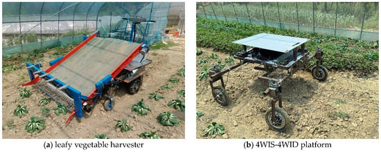
Figure 1. Experimental platforms.

2.2. Control System

The coordinated control system consists of the master control system, the slave control system, and the wireless communication system between the master and slave machines. Both the master and slave agricultural machine control systems are composed of a positioning and attitude measurement module and a navigation module. The positioning and attitude measurement module employs the PA-3 model RTK-GNSS (Huace Navigation Technology Ltd., Shanghai, China) and the WT901C model IMU sensor (Witmotion, Shenzhen, China). Due to the limitations of the modules and sensors, the sampling frequency of the pose information is 10 Hz. The navigation module uses the STM32F103ZET6 (STMicroelectronics, Geneva, Switzerland) as the core board, with software development and debugging carried out using Clion (JetBrains, Prague, Czech Republic) and STM32CubeMX (STMicroelectronics, Geneva, Switzerland). The wireless communication module is based on Wi-Fi for dual-machine communication.

The architecture of the coordinated control system is shown in Figure 2. First, the master PC receives the latitude and longitude information from the RTK-GNSS and converts it into position coordinates (x_M, y_M) in a specific coordinate system. The slave obtains its position coordinates (x_S, y_S) in the same manner. Next, the master’s main control unit, STM32F103ZET6, receives the (x_S, y_S) coordinates transmitted by the Wi-Fi module and sends them to the master PC. The coordinates (x_M, y_M) and (x_S, y_S) are further processed by an adder to calculate the master speed v_M and the relative distance d_p between the two vehicles. Then, the master speed v_M, relative distance d_p, and the master acceleration a_M from the IMU are decomposed into multiple IMF components using VMD. These components are input into the Transformer-LSTM model to predict the future speed sequence v_M(k)…v_M(k + N_p − 1). After the predicted sequence is transmitted to the master’s main control unit, it is further sent via the Wi-Fi module to the slave’s main control unit, STM32F103ZET6. Finally, the upper-level MPC of the slave outputs the reference speed v_ref(k)…v_ref(k + N_p – 1) based on v_M(k)…v_M(k + N_p – 1). The lower-level MPC calculates the final slave speed v_S based on v_ref(k)…v_ref(k + N_p – 1) and inputs it into the slave’s driving system.

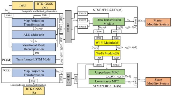
Figure 2. Coordinated control system architecture.

2.3. Algorithm Overview

The coordinated harvesting operation of the master and slave agricultural machines is generally divided into scheduling coordination and following coordination [27]. Scheduling coordination refers to the process where when the master is at full capacity, an unloading request signal is sent to the slave. Upon receiving the signal, the slave immediately plans the optimal path and autonomously navigates to the master’s location to complete precise docking and material transfer operations. Tracking coordination refers to the process where the slave always follows the master’s movement trajectory and speed during operation, maintaining a stable relative position to achieve seamless material transfer. Both methods can be applied in grain harvesting operations because the harvester itself has some storage capacity. However, the furrow surface of leafy vegetable harvesters cannot bear too much weight, so their storage capacity is limited. Therefore, leafy vegetable coordinated harvesting includes both scheduling and following operation modes.

The locations of ridge-cultivated vegetables and agricultural machinery storage areas in the facility environment are shown in Figure 3, and a coordinate system is established.

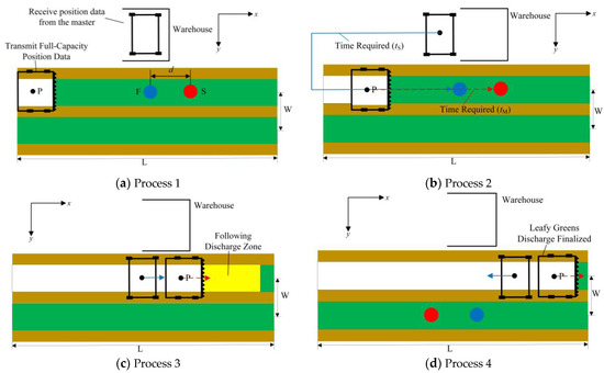
Figure 3. Master-Slave collaborative harvesting schematic. Note: L is the length of the vegetable bed ridge; W is the width of the vegetable bed ridge.

Step 1: At the current operation time i, the master machine is located at point P. The estimated full warehouse point M’s position is calculated and its location information is sent to the slave machine in the warehouse via the Wi-Fi module. When the slave machine follows the master machine for unloading operations, the optimal distance between the two machines is d.

Step 2: Let the travel time of the slave machine from the warehouse to point F be t_S, and the travel time from the current position of the slave machine to point S be t_M. t_M decreases continuously from time i, and when t_S equals t_M, the slave machine departs from the warehouse and heads toward point F.

Step 3: After the master and slave machines reach their designated positions, both machines enter a continuous follow-and-unload mode without stopping.

Step 4: After unloading is completed, the slave machine returns to the warehouse, while the master machine continues harvesting and calculates the location information of the next full warehouse point, which is then sent to the slave machine waiting in the warehouse, thus completing the cyclical collaborative operation.

Master–slave tracking is a key process in leafy vegetable coordinated harvesting. High-precision following can reduce the motion delay between the Master and Slave, preventing repeated adjustments or harvesting pauses caused by position errors, thereby improving the efficiency of continuous operations. Therefore, the accuracy of master–slave tracking directly determines the effectiveness of leafy vegetable coordinated harvesting.

2.4. Master Speed Prediction

2.4.1. Master Speed Prediction Process

The effective prediction of v_M(k)…v_M(k + N_p – 1) is a prerequisite for achieving high-precision master–slave tracking. The master speed prediction in this paper is divided into three steps. The prediction process is shown in Figure 4.

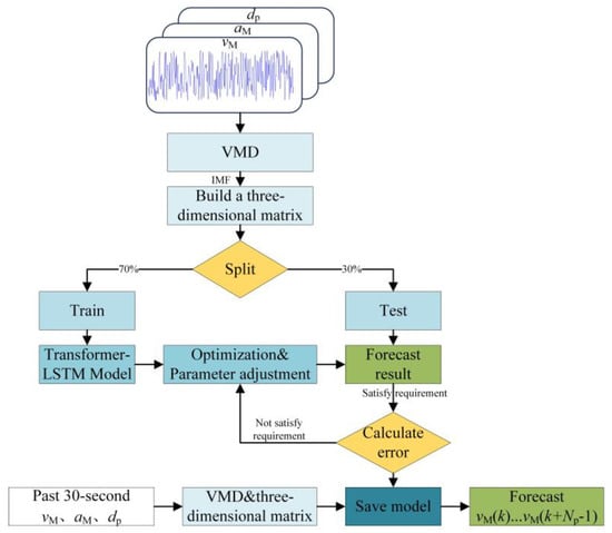
Figure 4. Master speed prediction process.

Step 1: The leafy vegetable harvester operates in the field at a speed of 0.6 m/s. The 4WIS-4WID platform follows the harvester at a distance of 0.5 m behind, moving at the same speed. The speed, acceleration, and relative distance between the two machines are collected in real time, and these data are used to form the datasets for v_M, a_M, and d_p.

Step 2: VMD is used to decompose v_M, a_M, and d_p into multiple IMF. The non-uniform IMF sequences are then reconstructed into a regularized three-dimensional matrix. This matrix is subsequently input into the Transformer-LSTM model for training, and the trained model is saved.

Step 3: During coordinated harvesting, the past 30 s of v_M, a_M, and d_p are processed through VMD and used to construct a three-dimensional matrix. This matrix is then input into the saved model, which outputs v_M(k)…v_M(k + N_p – 1).

2.4.2. Variational Mode Decomposition

(a)

Decomposition Principle

Before the information is input into the prediction model, preprocessing is performed to effectively improve prediction accuracy and computational efficiency. Variational Mode Decomposition (VMD) [28,29] demonstrates strong robustness when handling nonlinear and non-stationary signals, effectively avoiding the occurrence of spurious components during decomposition. Therefore, this paper uses VMD to decompose v_M, a_M, and d_p into multiple IMF.

The VMD process is as follows:

Step 1: The analytic signal related to the decomposition is calculated through the Hilbert transform [30], and the frequency spectrum is constructed. The estimated center frequency is then used to shift the modal spectrum to the baseband.

Step 2: A regularization constraint function is defined to constrain the bandwidth width of each component. By performing L₂ regularization on the gradient of the demodulated signal and using Gaussian smoothing estimates, the bandwidth of each v_M, a_M, and d_p data is obtained. The constraint variational problem generated in this step can be expressed as:

$$\left\{\begin{array}{c}{\min }_{\left\{c_h\right\},\left\{{\omega }_h\right\}}\left\{{{\displaystyle \sum }}_{h=1}^h\parallel {\partial }_{\mathrm{t}}\left[\left(\delta (\mathrm{t})+{\displaystyle \frac{\mathrm{j}}{\pi \mathrm{t}}}\right)\otimes c_h(\mathrm{t})\right]{\mathrm{e}}^{-\mathrm{j}{\omega }_h\mathrm{t}}{\parallel }_2^2\right\}\\ \mathrm{s}.\mathrm{t}.{{\displaystyle \sum }}_{h=1}^h{c}_h(\mathrm{t})=f(\mathrm{t})\end{array}\right.$$

(1)

In the equation, h represents the number of decompositions, c_h(t) denotes the h-th IMF component, ${\partial }_{\mathrm{t}}$ represents derivative with respect to time, ω_h is the center frequency of the h-th IMF, δ(t) represents the unit impulse function, ⊗ denotes the convolution operator, and f(t) refers to the original information of v_M, a_M, and d_p.

Step 3: A second-order penalty factor α and Lagrange multiplier λ(t) are introduced to obtain a new augmented Lagrangian optimization model, expressed as follows:

$$\begin{array}{l}\mathcal{L}(\{c_h\},\{{\omega }_h\},\lambda )=\alpha {\displaystyle \sum _h{‖\left[{\delta }_{\mathrm{t}}\left(\delta (\mathrm{t})+\frac{\mathrm{j}}{\pi \mathrm{t}}\right)\otimes c_h(\mathrm{t})\right]{\mathrm{e}}^{-\mathrm{j}{\omega }_h\mathrm{t}}‖}_2^2}\\ +{‖f(\mathrm{t})-{\displaystyle \sum _h{c}_h}(\mathrm{t})‖}_2^2+⟨\lambda (\mathrm{t}),f(\mathrm{t})-{\displaystyle \sum _h{c}_h}(\mathrm{t})⟩\end{array}$$

(2)

Step 4: The Alternating Direction Method of Multipliers (ADMM) is used to solve for the relative information data components c_h of each master–slave pair and their corresponding center frequencies ω_h. The specific procedure is as follows:

$${\hat{c}}_h^{(m+1)}(\omega )={\displaystyle \frac{\hat{r}(\omega )-{{\displaystyle \sum }}_{\mathrm{i}\ne h}{\hat{c}}_h^{(m)}(\omega )+\frac{{\hat{\lambda }}^{(m)}(\omega )}{2}}{1+2\alpha {\left(\omega -{\omega }_h^{(m)}\right)}^2}}$$

(3)

$${\omega }_h^{(m+1)}={\displaystyle \frac{{{\displaystyle \int }}_0^{\infty }\omega \mid {\hat{c}}_h^{(m+1)}(\omega ){\mid }^2\mathrm{d}\omega }{{{\displaystyle \int }}_0^{\infty }\mid {\hat{c}}_h^{(m+1)}(\omega ){\mid }^2\mathrm{d}\omega }}$$

(4)

In the equation, r(ω), c_h(ω) and λ(ω) represent the Fourier transforms of r(t), c_h(t) and λ(t), respectively; ω is the frequency; and h is the number of iterations for the variational model search.

(b)

Selection of the Number h of Components

When decomposing the signals of v_M, a_M, and d_p, the number of components h has a significant impact on the decomposition results. A value of h that is too large may lead to over-decomposition and model overfitting, while a value that is too small may result in under-decomposition. Therefore, selecting an appropriate value for h is crucial for obtaining accurate prediction results. In this paper, the center frequency method is used to determine the number of components h. Specifically, the center frequencies of the components are calculated for values of h in the set {3, 4, 5, 6, 7, 8}. If there are similar components, it indicates over-decomposition.

Here, the training set of v_M is used as an example. As shown in Figure 5, the master’s v_M exhibits significant randomness and nonstationarity. Then, VMD processing is applied to the data in Figure 5 for different values of h, and the center frequencies of each IMF component are shown in Table 1.

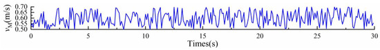
Figure 5. Example of Master historical speed.

Table 1. Center frequencies of v_M’s IMF components under different h values.

h	IMF1/Hz	IMF2/Hz	IMF3/Hz	IMF4/Hz	IMF5/Hz	IMF6/Hz	IMF7/Hz	IMF8/Hz
3	0.3729	0.1525	0
4	0.3729	0.2034	0.1186	0
5	0.3831	0.3051	0.2034	0.1186	0
6	0.4407	0.3729	0.2034	0.1525	0.0746	0
7	0.4407	0.3729	0.3051	0.2034	0.1525	0.0746	0
8	0.4407	0.3729	0.3051	0.2373	0.2034	0.1525	0.0746	0

As shown in Table 1, when h = 8, two IMF components with center frequencies of 0.2034 Hz and 0.2373 Hz are found to be similar, indicating over-decomposition. Therefore, h is determined to be 7, and the VMD result is shown in Figure 6.

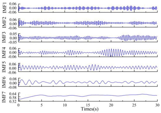
Figure 6. VMD decomposition results of the v_M.

Similarly, the VMD results for a_M and d_p are obtained, as shown in Figure 7a and Figure 7b, respectively.

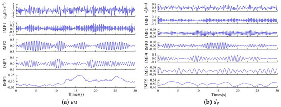
Figure 7. VMD decomposition results.

2.4.3. Transformer-LSTM Prediction Model

The IMF components of v_M, a_M and d_p after VMD have different frequencies. The period length of the high-frequency IMF is not fixed, and most of the important features are concentrated at a few time points, with the remaining parts noise-resembling. The low-frequency IMF exhibit a slow-changing trend, with the main information distributed throughout the entire sequence and minimal noise.

The master–slave tracking requires the model to adjust the slave’s speed in real-time based on changes in v_M, a_M and d_p, in order to ensure efficient and accurate tracking operations. Due to the complex dynamic features and long-term dependencies involved in this task, a single prediction model may struggle to handle the fusion and extraction of multi-frequency information. The Transformer model, with its multi-head attention mechanism [30,31,32], effectively captures transient correlations between different variables and the impact of early data changes on the later behavior of v_M. The LSTM model, with its unique gating mechanism, selectively remembers long-term features of the data, making it better suited for capturing low-frequency temporal information [33]. Therefore, by inputting high-frequency IMF into the Transformer model to extract global features, and low-frequency IMF into the LSTM model to extract temporal features, we can better predict the dynamic variations in different frequencies in the master–slave tracking process, providing more accurate future speed sequences for the master machine, and thereby offering more reliable support for the harvesting control system.

Therefore, in this paper, the first three sets of IMF components are input into the Transformer model to extract the high-frequency features of the data, while the remaining four sets of IMF components are input into the LSTM model to extract the low-frequency features. The feature results from both models are then concatenated, and the speed prediction results are output. The network structure of the Transformer-LSTM model is shown in Figure 8.

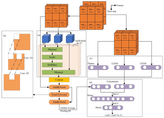
Figure 8. Network architecture of the Transformer-LSTM model. (a) Transformer model. (b) feed-forward neural network. (c) LSTM model. (d) Integration phase.

The multi-head attention mechanism in the Transformer model is shown in Figure 8a, and its principle is as follows.

First, the input matrix is transformed three times to generate the query matrix Q, key matrix K, and value matrix V. Then, Q, K, and V continuously interact under the self-attention mechanism. Finally, the different attention results are concatenated. The mathematical expression is as follows:

$$\mathrm{MulitHead}(Q,K,V)=\mathrm{Concat}({head}_1,\dots ,{head}_{\mathrm{h}})$$

(5)

$${head}_{\mathrm{i}}=\mathrm{Attention}\left(Q{W}_i^Q,K{W}_i^K,V{W}_i^V\right)$$

(6)

where $W_i^Q$, $W_i^K$, $W_i^V$ are the linear transformation weight matrices for the i-th head, and the dynamic allocation of weights is given by the following Equation (7):

$$\mathrm{Attention}(Q,K,V)=\mathrm{softmax}\left({\displaystyle \frac{Q{K}^T}{\sqrt{d_k}}}\right)V$$

(7)

The multi-head attention mechanism can lead to the loss of original information, while residual connections help maintain the flow of input information without introducing additional data. To better preserve the original input information, as shown in Figure 8b, the output of the multi-head attention mechanism is combined with the original input through a residual connection. After the residual connection, two 1D convolutional layers form a feed-forward neural network, which enhances the model’s ability to capture local features. To ensure a fixed sequence length, the output processed by the feed-forward neural network is subjected to global average pooling. Finally, the original input is concatenated with the output after global average pooling. The concatenated data is then passed through a fully connected layer with 32 neurons and a ReLU activation function for feature integration.

The network structure for processing low-frequency IMFs with LSTM is shown in Figure 8c. The model uses two parallel LSTM layers, allowing the model to capture global features while also considering local features, thereby providing more comprehensive feature information for the next layer. The two LSTM layers are flattened with the original input data for feature fusion. Finally, the output data is connected to a fully connected layer with 32 neurons. Each LSTM layer controls the flow of information through its gating mechanism, and the computation process is as follows:

$$f_{\mathrm{t}}=\sigma \left(W_f\cdot \left[h_{\mathrm{t}-1},x_{\mathrm{t}}\right]+b_f\right)$$

(8)

$$i_{\mathrm{t}}=\sigma \left(W_i\cdot \left[h_{\mathrm{t}-1},x_{\mathrm{t}}\right]+b_i\right)$$

(9)

$${\hat{C}}_{\mathrm{t}}=\tanh \left(W_C\cdot \left[h_{\mathrm{t}-1},x_{\mathrm{t}}\right]+b_C\right)$$

(10)

$$C_{\mathrm{t}}=f_{\mathrm{t}}\cdot C_{\mathrm{t}-1}+i_{\mathrm{t}}\cdot {\hat{C}}_{\mathrm{t}}$$

(11)

$$o_{\mathrm{t}}=\sigma \left(W_o\cdot \left[h_{\mathrm{t}-1},x_{\mathrm{t}}\right]+b_o\right)$$

(12)

$$h_{\mathrm{t}}=o_{\mathrm{t}}\cdot \tanh (C_{\mathrm{t}})$$

(13)

In the equation, f_t, i_t, o_t represent the forget gate, input gate, and output gate, respectively; C_t is the current memory cell state; and h_t is the hidden state at the current time step.

As shown in Figure 8d, after the Transformer and LSTM models output their features, the output features of both are concatenated and used as the input to the Transformer-LSTM. The Transformer-LSTM consists of fully connected neural networks. Considering the model’s simplicity, stability, and non-linearity, three fully connected layers are constructed in the model, with 64, 64, and 32 neurons, respectively.

2.4.4. Evaluation Metrics

To evaluate the performance of the VMD-Transformer-LSTM model, a series of evaluation metrics are selected: Root Mean Square Error (RMSE), Mean Absolute Error (MAE), Mean Absolute Percentage Error (MAPE), and Coefficient of Determination (R²). Among these metrics, a lower value of RMSE, MAE, and MAPE, along with a higher value of R², indicates higher prediction accuracy of the model. The calculation formulas are as follows:

$$\mathrm{RMSE}=\sqrt{{\displaystyle \frac{1}{n}}{\displaystyle \sum }_{i=1}^n{\left[v_{\mathrm{M}}(i)-{\hat{v}}_{\mathrm{M}}(i)\right]}^2}$$

(14)

$$\mathrm{MAE}={\displaystyle \frac{1}{n}}{\displaystyle \sum }_{i=1}^n\mid v_{\mathrm{M}}(i)-{\hat{v}}_{\mathrm{M}}(i)\mid$$

(15)

$$\mathrm{MAPE}={\displaystyle \frac{1}{n}}{\displaystyle \sum }_{i=1}^n\mid {\displaystyle \frac{v_{\mathrm{M}}(i)-{\hat{v}}_{\mathrm{M}}(i)}{v_{\mathrm{M}}(i)}}\mid \times 100\%$$

(16)

$$R^2=1-{\displaystyle \frac{{{\displaystyle \sum }}_{i=1}^n{\left[v_m(i)-{\hat{v}}_m(i)\right]}^2}{{{\displaystyle \sum }}_{i=1}^n{\left[v_m(i)-{\overline{v}}_m\right]}^2}}$$

(17)

In the equation, n is the total number of samples; $v_{\mathrm{M}}(i)$ is the actual value of the i-th sample; ${\hat{v}}_{\mathrm{M}}(i)$ is the predicted value of the i-th sample; and ${\overline{v}}_m$ is the average value of the master speed.

2.5. Slave Speed Control

2.5.1. Dual-Layer MPC

Combined with the master speed prediction, a slave speed control strategy using dual-layer MPC is developed to achieve higher precision in master–slave tracking. The specific structure is shown in Figure 9. Considering the real-time requirements of speed control, an MPC based on a discrete state-space model is used, as detailed below. At time k, the relative distance d_p and the velocity error (v_e) between the master and slave are used as state variables x(k), represented as [v_e; d_p]. The slave acceleration a_S and the slave final speed v_S are taken as control variables u(k) and output variables y(k), denoted as [a_S; v_S]. Both layers of the MPC receive the current system state x(k) and the future speed sequence of length N_p output by the master speed prediction model, which has strict temporal sequencing.

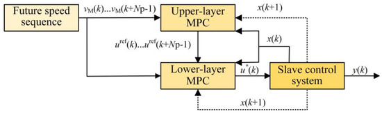
Figure 9. Schematic diagram of dual-layer MPC.

The slave speed control method in this paper is divided into two parts. First, the upper-layer MPC, based on the current state x(k) and the master’s future speed sequence, aims to minimize the velocity error between the master and slave. This results in a control variable sequence u(k)…u(k + N_P − 1), which then outputs the reference speed v_ref for N_p steps. Then, the lower-layer MPC, based on x(k) and v_ref, aims to minimize the relative distance error between the master and slave. The first control variable u*(k) of length N_p is applied to the slave’s driving system to achieve the final slave speed control. At the same time, the updated x(k + 1) is fed back to the MPC for speed control at time k + 1. The entire model continuously repeats this process in a recursive manner.

The MPC based on the discrete state-space model is given by Equations (18) and (19).

$$\left\{\begin{array}{l}x(k+1)=Ax(k)+Bu(k)\\ y(k)=Cx(k)+Du(k)\end{array}\right.$$

(18)

In the equations, A, B, and C are the coefficient matrices of the discrete state-space equations; x(k), u(k), y(k) represent the state variables, control variables, and output variables at time k, respectively. D is the feedforward matrix. Due to the inherent inertia or delay in system dynamics, the control input does not instantaneously affect the output. Additionally, to simplify the derivation of the prediction equations and the construction of the optimization problem, as well as to improve numerical stability, this study sets D to zero vector.

$$\begin{array}{l}X(k+1)=\left[\begin{array}{c}A\\ A^2\\ ⋮\\ A^{N_{\mathfrak{p}}}\end{array}\right]x(k)+\left[\begin{array}{cccc}B& & & \\ AB& B& & \\ ⋮& ⋮& \ddots & \\ A^{N_{\mathfrak{p}}-1}B& A^{N_{\mathfrak{p}}-2}B& \dots & B\end{array}\right]U(k)\\ X(k+1)=\left[\begin{array}{c}{x}_{k+1\mid k}\\ x_{k+2\mid k}\\ ⋮\\ x_{k+N_{\mathfrak{p}}\mid k}\end{array}\right],U(k)=\left[\begin{array}{c}{u}_{k\mid k}\\ u_{k+1\mid k}\\ ⋮\\ u_{k+N_{\mathfrak{p}}-1\mid k}\end{array}\right]\end{array}$$

(19)

In the equations, A ∈ R^nx×nx, B ∈ R^nx×nu, X(k) ∈ R^{(Npnx) × 1}, U(k) ∈ R^{(Npnu) × 1}; X(k) and U(k) are the state variable matrix and control variable matrix for the N_p steps at time k, respectively; x_k+1|k and u_k+1|k are the predicted state variables and control variables at time k + 1, respectively, based on the prediction at time k.

2.5.2. Upper-Layer MPC Constraints

The upper-layer MPC applies the optimized control variable sequence u(k), u(k + 1)…u(k + N_P − 1) to the slave control system. Then, the output reference speed sequence v_ref(k), v_ref(k + 1)…v_ref(k + N_P − 1) is passed to the lower-layer MPC as the reference speed sequence for the master. The optimization goal of the upper-layer MPC is to reduce the velocity error between the slave and the master. Therefore, the cost function f_U of the upper-layer MPC is given by Equation (20).

$$f_{\mathrm{U}}={\displaystyle \sum }_{j=k}^{k+N\mathrm{p}-1}{({\nu }_{\mathrm{M}}(j)-{\nu }_{\mathrm{S}})}^2$$

(20)

In the equation, j represents the time step.

2.5.3. Lower-Layer MPC Constraints

The lower-layer MPC optimizes the final output slave speed v_S based on x(k), v_ref, and the future speed sequence. The first control variable u*(k) within the N_p predicted steps is applied to the slave control system, outputting the final control signal y(k). The optimization goal of the lower-layer MPC is to minimize the relative distance error d_e between the master and slave, based on the slave speed matching the master’s predicted speed. Therefore, the cost function f_L of the lower-layer MPC is given by Equation (21).

$$f_{\mathrm{L}}={\displaystyle \sum }_{j=k}^{k+N\mathrm{p}-1}{\left({\displaystyle \frac{d_{\mathrm{e}}(j)}{\mathrm{e}{d}_{\mathrm{p}}}}\right)}^2$$

(21)

In the equation, ed_p is the desired relative longitudinal distance.

3. Results and Discussion

3.1. Experimental Scenario

To verify the feasibility of the proposed method in practical leafy vegetable coordinated harvesting, experiments were conducted from March to April 2025 at the Agricultural Experiment Base of Donghu Campus, Zhejiang A&F University, Hangzhou, China (30.2622° N, 119.7283° E). The experiments included master speed prediction, slave tracking, and coordinated harvesting operation tests. The greenhouse utilizes plastic film materials with excellent wave permeability. Tests have demonstrated that GNSS signals remain strong, with no observed degradation in positioning accuracy or continuity due to signal obstruction. The experimental scenario is shown in Figure 10.

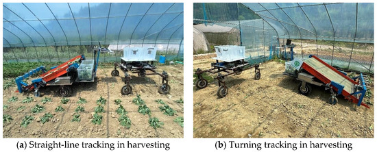
Figure 10. Experimental scenario of collaborative harvesting.

3.2. Master Speed Prediction Experiment

3.2.1. Experimental Design

The purpose of this experiment is to verify the prediction accuracy of the proposed VMD-Transformer-LSTM model for master speed during leafy vegetable harvesting, providing reliable baseline data for the subsequent slave-tracking control.

The speed prediction experiment was conducted using a leafy vegetable harvester in the field, and comparison tests were performed with the LSTM model, Transformer model, and Transformer-LSTM model.

3.2.2. Experimental Results

The speed prediction results of the four models during harvesting are shown in Figure 11.

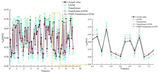
Figure 11. Prediction performance comparison.

To further assess the prediction accuracy, the performance and feasibility of the model in predicting master speed are evaluated by comparing the values of RMSE, MAE, MAPE, and R². The predicted data is shown in Table 2.

Table 2. Model accuracy data.

Model	LSTM	Transformer	Transformer-LSTM	VMD-Transformer-LSTM
MAE	0.0193	0.0267	0.0128	0.0107
MAPE	3.24%	4.51%	2.16%	1.79%
RMSE	0.0241	0.0333	0.0163	0.0136
R2	87.84%	76.89%	92.57%	94.81%

The predictive results were subjected to analysis of variance (ANOVA) and post hoc tests, with the outcomes presented in Table 3.

Table 3. ANOVA and Post Hoc Analysis.

Paired Variables	Mean Difference	p	Cohen’s d	Lower Bound of the 95%CI	Upper Bound of the 95%CI
LSTM vs. VMD-Transformer-LSTM	0.022	<0.001	1.67	0.0193	0.0248
Transformer vs. VMD-Transformer-LSTM	0.024	<0.001	1.45	0.0208	0.0277
Transformer-LSTM vs. VMD-Transformer-LSTM	0.007	<0.001	0.70	0.0046	0.0085

3.2.3. Data Analysis

As shown in Table 3 and Figure 11, the prediction accuracy of the LSTM and Transformer models is significantly lower than that of the other two models. By zooming in on the prediction results, it can be observed that the improved VMD-Transformer-LSTM model consistently provides predictions that are much closer to the actual master speed at any given time. VMD-Transformer-LSTM was compared with LSTM, Transformer, and Transformer-LSTM. The p-values were all less than 0.001, indicating that the differences between VMD-Transformer-LSTM and the other three models were statistically significant and not due to random chance. Compared to the first two models, the Cohen’s d values were greater than 0.8, suggesting a substantial magnitude of performance improvement. Although the Cohen’s d value was 0.7 when compared to Transformer-LSTM, it still represents a considerable effect size, demonstrating that incorporating VMD preprocessing leads to a significant enhancement. The comparison of confidence intervals shows that, for all three comparisons involving VMD-Transformer-LSTM, the entire intervals are far from zero, further confirming that the performance of VMD-Transformer-LSTM is significantly superior to that of the other three models.

As shown in Table 2, the MAE, MAPE, and RMSE of the three models are ranked as follows: VMD-Transformer-LSTM model > Transformer-LSTM model > Transformer model > LSTM model. Compared to the traditional LSTM, Transformer, and Transformer-LSTM models, the VMD-Transformer-LSTM model reduced MAE by 44.56%, 59.93%, and 16.41%, respectively; MAPE by 44.75%, 60.31%, and 17.13%, respectively; and RMSE by 43.57%, 59.16%, and 16.56%, respectively. These results demonstrate that the VMD-Transformer-LSTM model achieves the highest prediction accuracy.

It can also be observed from Table 2 that the R² values of the Transformer-LSTM model and the VMD-Transformer-LSTM model are both greater than 0.9. The R² of the VMD-Transformer-LSTM model is significantly higher than that of the LSTM, Transformer, and Transformer-LSTM models, with improvements of 6.97%, 17.92%, and 2.24%, respectively. These results all demonstrate that the VMD-Transformer-LSTM model has significantly better explanatory power over the independent variables compared to the traditional models. In conclusion, the VMD-Transformer-LSTM model proposed in this paper can provide a reliable future master speed sequence for slave-tracking control.

3.3. Slave Following Experiment

3.3.1. Experimental Design

The slave-tracking experiment aims to verify the tracking accuracy and stability of the proposed algorithm during leafy vegetable collaborative harvesting operations, providing key technical support for the master-slave cooperative harvesting system. Both the master and slave use a pure pursuit control algorithm to move autonomously in the field at a constant speed of 0.6 m/s. The slave adjusts its speed in real time using the control algorithm proposed in this paper to maintain the preset relative distance between the two machines. The experiment is divided into two groups: straight-line tracking (to evaluate steady-state tracking performance) and turning-tracking (to assess dynamic path adaptation capability). Each group of experiments is conducted three times and compared with the traditional MPC algorithm and the MPC algorithm with prediction.

3.3.2. Data Analysis

(a)

Straight-line Tracking

During straight-line tracking, the longitudinal distance between the two machines (the front-to-rear spacing in the direction of motion) is denoted as d_p. The results and data of the tracking experiment are shown in Figure 12 and Table 4. The obtained data were subjected to t-test, as shown in Table 5.

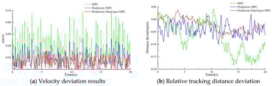
Figure 12. Results of straight-line tracking experiment.

Table 4. Straight-Line tracking error analysis.

Evaluation Metrics	MPC	Prediction + MPC	Prediction + Dual-Layer MPC
average speed deviation (m/s)	0.036	0.019	0.007
Maximum distance deviation (m)	0.185	0.101	0.068
average distance deviation (m)	0.077	0.041	0.028
average speed deviation (m/s)	0.032	0.017	0.008
Maximum distance deviation (m)	0.179	0.099	0.071
average distance deviation (m)	0.074	0.038	0.029
average speed deviation (m/s)	0.039	0.022	0.006
Maximum distance deviation (m)	0.192	0.124	0.063
average distance deviation (m)	0.081	0.049	0.025

Table 5. Straight-Line tracking error t-test.

	Paired Variables	Pairing Value 1	Pairing Value 2	p	Cohen’s d
speed deviation	MPC vs. Prediction + dual-layer MPC	0.0357 ± 0.0035	0.0070 ± 0.0010	<0.001	1.463
	Prediction + MPC vs. Prediction + dual-layer MPC	0.0193 ± 0.0025	0.0070 ± 0.0010	<0.001	0.891
distance deviation	MPC vs. Prediction + dual-layer MPC	0.0773 ± 0.0035	0.0273 ± 0.0021	<0.001	1.335
	Prediction + MPC vs. Prediction + dual-layer MPC	0.0427 ± 0.0055	0.0273 ± 0.0021	<0.001	0.885

(b)

Turning tracking

During turning tracking, the Manhattan distance between the two machines (the sum of the absolute distances in the lateral and longitudinal directions) is denoted as d_p. The results and data of the tracking experiment are shown in Figure 13 and Table 5. The results of the t-test are shown in Table 7.

Table 6. Turning tracking error analysis.

Evaluation Metrics	MPC	Prediction + MPC	Prediction + Dual-Layer MPC
average speed deviation (m/s)	0.052	0.032	0.014
Maximum distance deviation (m)	0.234	0.176	0.126
average distance deviation (m)	0.092	0.078	0.047
average speed deviation (m/s)	0.050	0.037	0.015
Maximum distance deviation (m)	0.249	0.179	0.137
average distance deviation (m)	0.097	0.083	0.049
average speed deviation (m/s)	0.054	0.030	0.014
Maximum distance deviation (m)	0.202	0.174	0.118
average distance deviation (m)	0.091	0.076	0.045

Table 6. Turning tracking error analysis.

Evaluation Metrics	MPC	Prediction + MPC	Prediction + Dual-Layer MPC
average speed deviation (m/s)	0.052	0.032	0.014
Maximum distance deviation (m)	0.234	0.176	0.126
average distance deviation (m)	0.092	0.078	0.047
average speed deviation (m/s)	0.050	0.037	0.015
Maximum distance deviation (m)	0.249	0.179	0.137
average distance deviation (m)	0.097	0.083	0.049
average speed deviation (m/s)	0.054	0.030	0.014
Maximum distance deviation (m)	0.202	0.174	0.118
average distance deviation (m)	0.091	0.076	0.045

Figure 13. Results of turning tracking experiment.

Table 7. Turning tracking error t-test.

	Paired Variables	Pairing Value 1	Pairing Value 2	p	Cohen’s d
speed deviation	MPC vs. Prediction + dual-layer MPC	0.0520 ± 0.0020	0.0143 ± 0.0006	<0.001	1.167
	Prediction + MPC vs. Prediction + dual-layer MPC	0.0330 ± 0.0036	0.0143 ± 0.0006	<0.001	0.891
distance deviation	MPC vs. Prediction + dual-layer MPC	0.0933 ± 0.0031	0.0470 ± 0.0020	<0.001	0.898
	Prediction + MPC vs. Prediction + dual-layer MPC	0.0790 ± 0.0036	0.0470 ± 0.0020	0.003	0.485

Table 7. Turning tracking error t-test.

	Paired Variables	Pairing Value 1	Pairing Value 2	p	Cohen’s d
speed deviation	MPC vs. Prediction + dual-layer MPC	0.0520 ± 0.0020	0.0143 ± 0.0006	<0.001	1.167
	Prediction + MPC vs. Prediction + dual-layer MPC	0.0330 ± 0.0036	0.0143 ± 0.0006	<0.001	0.891
distance deviation	MPC vs. Prediction + dual-layer MPC	0.0933 ± 0.0031	0.0470 ± 0.0020	<0.001	0.898
	Prediction + MPC vs. Prediction + dual-layer MPC	0.0790 ± 0.0036	0.0470 ± 0.0020	0.003	0.485

3.3.3. Data Analysis

(a)

Straight-line Tracking

As shown in Table 5, when comparing traditional MPC with the dual-layer MPC incorporating a prediction model, the p-values for both speed deviation and distance deviation are less than 0.001, indicating a statistically significant difference between the two approaches. The corresponding Cohen’s d values, 1.463 and 1.335, further suggest a very large effect size. Similarly, when comparing the MPC with a prediction model and the dual-layer MPC with a prediction model, the p-values for both speed and distance deviations are also less than 0.001, and the Cohen’s d values are greater than 0.8, demonstrating not only statistical significance but also a substantial magnitude of difference.

As shown in Figure 11 and Figure 12a, the improved algorithm in this paper significantly enhances the ability to control the speed error between the master and slave machines. On one hand, the VMD-Transformer-LSTM model is used to predict the future speed of the master, avoiding the drawback of not being able to obtain the master speed in a timely manner. On the other hand, the upper-layer MPC ensures that the slave speed is closer to the master speed.

In terms of master-slave tracking accuracy, the traditional MPC algorithm shows a relatively large tracking error, with an average speed deviation of 0.036 m/s, an average distance deviation of 7.7 cm, and a maximum distance deviation of 19.2 cm. On the other hand, the MPC algorithm with the prediction model significantly reduces the tracking error, with an average speed deviation of 0.019 m/s, an average distance deviation of 4.3 cm, and a maximum distance deviation of 12.4 cm. These values represent reductions of 47.22%, 44.16%, and 35.42%, respectively, compared to the MPC algorithm without the prediction model. After applying the dual-layer MPC algorithm in this paper, the tracking error is further reduced, with an average speed deviation of 0.007 m/s, an average distance deviation of 2.7 cm, and a maximum distance deviation of 7.1 cm. These values represent reductions of 63.16%, 37.26%, and 42.74%, respectively, compared to the traditional MPC algorithm. These results all demonstrate the effectiveness of the proposed method in improving tracking accuracy.

As shown in Figure 12b, when using the improved algorithm for master-slave tracking, the relative deviation is significantly smaller and the variation is relatively stable. In contrast, when the traditional MPC algorithm is used for tracking, the relative distance deviation fluctuates greatly and is highly unstable. This is mainly due to the inability to accurately obtain the master machine’s speed, which results in an unstable relative distance between the two machines. When the traditional MPC algorithm with the prediction model is used for tracking, the relative distance is relatively stable, but it still exhibits continuous fluctuations. This is mainly because the lower-layer MPC not only makes the slave speed closer to the master speed, but also minimizes the distance deviation as its objective, thereby generating the final speed control signal.

(b)

Turning Tracking

Similar to the straight-line tracking experiment, the method combining the VMD-Transformer-LSTM model and the dual-layer MPC can also effectively reduce the speed and relative distance errors between the master and slave machines in the turning-tracking experiment.

As can be seen from Table 7, when comparing traditional MPC with the dual-layer MPC incorporating a prediction model, the p-values for both speed and distance deviations are less than 0.001, and the Cohen’s d values are greater than 0.8, indicating a statistically significant difference between the two with a very large effect size. When comparing MPC with a prediction model and dual-layer MPC with a prediction model, the p-values for speed deviation are less than 0.001, and the Cohen’s d values are greater than 0.8, demonstrating a statistically significant difference with a very large effect size. For distance deviation, the Cohen’s d value is 0.485, suggesting a small effect size, while the p-value is 0.003, indicating that the difference remains statistically significant.

As shown in Figure 13 and Table 6, in terms of master-slave tracking accuracy, the traditional MPC algorithm exhibits a large tracking error, with an average speed deviation of 0.052 m/s, an average distance deviation of 9.3 cm, and a maximum longitudinal distance deviation of 24.9 cm. The MPC algorithm with the prediction model significantly reduces the tracking error, with an average speed deviation of 0.033 m/s, an average longitudinal distance deviation of 7.9 cm, and a maximum longitudinal distance deviation of 17.9 cm. These values represent reductions of 36.54%, 15.05%, and 28.11%, respectively, compared to the MPC algorithm without the prediction model. After applying the dual-layer MPC algorithm in this paper, the tracking error is further reduced, with an average speed deviation of 0.014 m/s, an average longitudinal distance deviation of 4.7 cm, and a maximum longitudinal distance deviation of 13.7 cm. These values represent reductions of 57.58%, 40.51%, and 23.46%, respectively, compared to the traditional MPC algorithm. Although the accuracy during turning-tracking has decreased slightly, the tracking performance is still superior to the traditional control algorithms.

Based on the results of the two experiments mentioned above, the improved algorithm in this paper achieves an average speed error of less than 0.007 m/s and a distance deviation of less than 7.1 cm for straight-line tracking. For turning-tracking, the average speed error is controlled within 0.014 m/s, and the distance deviation is kept within 13.7 cm. The tracking accuracy and stability show a significant improvement compared to the traditional algorithms, effectively meeting the precision requirements for leafy vegetable collaborative harvesting. Therefore, the algorithm proposed in this paper can be used as the control algorithm for leafy vegetable cooperative harvesting operations.

3.4. Collaborative Harvesting Operation Experiment

3.4.1. Experimental Design

The collaborative harvesting operation experiment aims to verify the efficiency of the method proposed in this paper during leafy vegetable collaborative harvesting. With the premise of ensuring master–slave tracking accuracy, the algorithm combining the VMD-Transformer-LSTM model and the dual-layer MPC is used as the primary control algorithm for the collaborative operation.

The collaborative harvesting method was tested three times and compared to the traditional harvesting method (waiting for the transport vehicle to unload after the grain tank is full, without the follow-up unloading process). The average operational efficiency of both methods was compared.

3.4.2. Experimental Results

The time information of the collaborative harvesting is shown in Table 8 and Figure 14.

Table 8. Time data for collaborative harvesting experiment.

Harvesting Model	Agricultural Machinery Categories	Average Non-Operating Time(s)	Average Total Time Consumption(s)
Traditional harvesting	Master	67	336
	Slave 1	85	346
	Slave 2	138	406
Master–slave tracking harvesting	Master	0	210
	Slave 1	44	269
	Slave 2	76	232

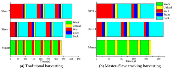
Figure 14. Coordinated harvesting experiment time window.

3.4.3. Data Analysis

Since this experiment only involved counting the number of harvesting cycles and the time consumed, and due to site limitations, it was not possible to conduct multiple trials, resulting in a relatively small dataset. However, the incorporation of the follow-and-unload process in our method is certain to reduce the total harvesting time to some extent. In all three trials that were carried out, the proposed method consistently demonstrated the advantages.

In terms of the slave workload, as shown in Figure 14, using the traditional leafy vegetable harvesting method, the slave is required to make 6 trips. However, with the method proposed in this paper, by adding the follow-and-unload process during the collaborative operation, the slave only needs to make 5 trips, thus saving the slave’s workload to some extent.

In terms of non-operating time, using the traditional leafy vegetable harvesting method, the non-operating times of slave 1 and slave 2 are 85 s and 138 s, respectively. However, with the leafy vegetable harvesting mode proposed in this paper, the non-operating times of slave 1 and slave 2 are reduced to 44 s and 76 s, respectively, representing reductions of 48.24% and 44.93% compared to the traditional harvesting mode. Using the method proposed in this paper, the leafy vegetable harvester can remain in a working state at all times, whereas in the traditional harvesting mode, the harvester experiences 67 s of non-operating time. This demonstrates that the method proposed in this paper can significantly improve the utilization of agricultural machinery.

In terms of total time, as shown in Table 8, using the traditional leafy vegetable harvesting mode, the total working time of the master is 336 s, while the total working times of slave 1 and slave 2 are 346 s and 406 s, respectively. With the method proposed in this paper, the total working time of the master is reduced to 210 s, and the total working times of slave 1 and slave 2 are 269 s and 232 s, respectively. Thus, compared to the traditional harvesting mode, the total working time of the master is reduced by 37.5%, while the total working times of slave 1 and slave 2 are reduced by 22.25% and 42.86%, respectively. This demonstrates that the method proposed in this paper can significantly improve work efficiency during leafy vegetable harvesting.

The harvesting experiment results show that the method proposed in this paper is effective in both reducing the workload of slaves and improving agricultural machinery utilization and leafy vegetable harvesting efficiency. In conclusion, the method proposed in this paper can be applied to practical leafy vegetable collaborative harvesting operations.

4. Conclusions

To address the challenge of accurately obtaining the master’s speed—caused by uneven terrain and varying soil hardness in farmland operations, which further leads to poor tracking performance of the slave—this study proposes a control method combining a VMD–Transformer–LSTM prediction model with a dual-layer MPC. The prediction model effectively forecasts future speed sequences of the master, while the dual-layer MPC accurately computes the required speed for the slave. Field experiments demonstrate that the VMD–Transformer–LSTM model can precisely predict the master’s speed, and its integration with the dual-layer MPC significantly improves the tracking accuracy between the master and slave. Furthermore, under the condition of ensuring master–slave tracking performance, a collaborative harvesting experiment for leaf vegetables was conducted using the proposed cooperative harvesting model. The results show that, compared with traditional collaborative harvesting methods, the proposed approach effectively reduces the number of transport vehicle operations, total working time, and non-working time. These findings indicate that the method successfully reduces the workload of transport vehicles, improves the utilization rate of agricultural machinery, and enhances the efficiency of leafy vegetable harvesting.

The leafy vegetable harvesting experiment has proven the feasibility of the method proposed in this paper for leafy vegetable collaborative harvesting. However, there are limitations in evaluating the factors influencing the master machine’s speed, as the agricultural environment is also an important factor affecting the master machine’s speed. For example, soil moisture, terrain undulations, and other factors. In this paper, these influencing factors were not considered when predicting the future speed of the master machine. In future work, it is planned to use multi-sensor fusion to gather various external influencing factors, further improving the accuracy of the prediction model.

References

- Li, H.; Zhong, T.; Zhang, K.; Wang, Y.; Zhang, M. Design of Agricultural Machinery Multi-machine Cooperative Navigation Service Platform Based on WebGIS. Trans. Chin. Soc. Agric. Mach. 2022, 53 (Suppl. S1), 28–35. [Google Scholar]
- Zhang, C.; Jia, L.; Liu, S.; Dou, G.; Liu, Y.; Kong, B. Dynamic job allocation method of multiple agricultural machinery cooperation based on improved ant colony algorithm. Sci. Rep. 2024, 14, 22414. [Google Scholar] [CrossRef]
- Guo, Y.; Zhang, F.; Chang, S.; Li, Z.; Li, Z. Research on a multiobjective cooperative operation scheduling method for agricultural machinery across regions with time windows. Comput. Electron. Agric. 2024, 224, 109121. [Google Scholar] [CrossRef]
- Yao, Z.; Zhao, C.; Zhang, T. Agricultural machinery automatic navigation technology. Iscience 2024, 27, 108714. [Google Scholar] [CrossRef]
- Zhang, M.; Li, X.; Wang, L.; Jin, L.; Wang, S. A Path Planning System for Orchard Mower Based on Improved A* Algorithm. Agronomy 2024, 14, 391. [Google Scholar] [CrossRef]
- Goodall, N.; Lan, C. Car-following characteristics of adaptive cruise control from empirical data. J. Transp. Eng. Part A Syst. 2020, 146, 04020097. [Google Scholar]
- Melson, C.; Levin, M.; Hammit, B.; Boyles, S. Dynamic traffic assignment of cooperative adaptive cruise control. Transp. Res. Part C Emerg. Technol. 2018, 90, 114–133. [Google Scholar]
- Wang, C.; Gong, S.; Zhou, A.; Li, T.; Peeta, S. Cooperative adaptive cruise control for connected autonomous vehicles by factoring communication-related constraints. Transp. Res. Part C Emerg. Technol. 2020, 113, 124–145. [Google Scholar] [CrossRef]
- Wu, X.; Yuan, C.; Shen, J.; Chen, L.; Cai, Y.; He, Y. Cooperative Control Research on Emergency Collision Avoidance of Human–Machine Cooperative Driving Vehicles. IEEE Trans. Veh. Technol. 2024, 73, 9632–9644. [Google Scholar] [CrossRef]
- Xu, G.; Chen, M.; Miao, H.; Yao, W.; Diao, P.; Wang, W. Following operation control method of farmer machinery based on model predictive control. Trans. Chin. Soc. Agric. Mach. 2020, 51 (Suppl. S2), 11–20. [Google Scholar]
- Ding, F.; Zhang, W.; Luo, X.; Hu, L.; Zhang, Z.; Wang, M.; Li, H.; Peng, M.; Wu, X.; Hu, L.; et al. Gain self-adjusting single neuron PID control method and experiments for longitudinal relative position of harvester and transport vehicle. Comput. Electron. Agric. 2023, 213, 108215. [Google Scholar] [CrossRef]
- Zhang, W.; Hu, L.; Ding, F.; Luo, X.; Zhang, Z.; Hu, L.; Huang, P.; Peng, M. Parking precise alignment control and cotransporter system for rice harvester and transporter. Comput. Electron. Agric. 2023, 215, 108443. [Google Scholar] [CrossRef]
- Roshanianfard, A.; Noguchi, N.; Okamoto, H.; Ishii, K. A review of autonomous agricultural vehicles (The experience of Hokkaido University). J. Terramech. 2023, 91, 155–183. [Google Scholar] [CrossRef]
- Mao, W.; Liu, H.; Hao, W.; Yang, F.; Liu, Z. Development of a combined orchard harvesting robot navigation system. Remote Sens. 2022, 14, 675. [Google Scholar] [CrossRef]
- Ma, Z.; Chong, K.; Ma, S.; Fu, W.; Yin, Y.; Yu, H.; Zhao, C. Control Strategy of Grain Truck Following Operation Considering Variable Loads and Control Delay. Agriculture 2022, 12, 1545. [Google Scholar] [CrossRef]
- Li, Y.; Yu, H.; Xiao, L.; Yuan, Y. Inspection robot GPS outages localization based on error Kalman filter and deep learning. Robot. Auton. Syst. 2025, 183, 104824. [Google Scholar] [CrossRef]
- Zhang, S.; Zhao, Z.; Wu, J.; Jin, Y.; Jeng, D.; Li, S.; Li, G.; Ding, D. Solving the temporal lags in local significant wave height prediction with a new VMD-LSTM model. Ocean. Eng. 2024, 313, 119385. [Google Scholar] [CrossRef]
- Zhang, X.; Hou, D.; Mao, Q.; Wang, Z. Predicting microseismic sensitive feature data using variational mode decomposition and transformer. J. Seismol. 2024, 28, 229–250. [Google Scholar] [CrossRef]
- Ding, Y.; Wang, L.; Li, Y.; Li, D. Model predictive control and its application in agriculture: A review. Comput. Electron. Agric. 2018, 151, 104–117. [Google Scholar] [CrossRef]
- Cáceres, G.; Millán, P.; Pereira, M.; Lozano, D. Smart farm irrigation: Model predictive control for economic optimal irrigation in agriculture. Agronomy 2021, 11, 1810. [Google Scholar] [CrossRef]
- Soitinaho, R.; Oksanen, T.; Pereira, M.; Lozano, D. Local Navigation and Obstacle Avoidance for an Agricultural Tractor With Nonlinear Model Predictive Control. IEEE Trans. Control Syst. Technol. 2023, 31, 2043–2054. [Google Scholar] [CrossRef]
- Lee, C.; Chung, D.; Kim, J.; Kim, J. Nonlinear model predictive control with obstacle avoidance constraints for autonomous navigation in a canal environment. IEEE/ASME Trans. Mechatron. 2023, 29, 1985–1996. [Google Scholar] [CrossRef]
- Nag, A.; Yamamoto, K. Distributed control for flock navigation using nonlinear model predictive control. Adv. Robot. 2024, 38, 619–631. [Google Scholar] [CrossRef]
- Knudsen, B.; Alessandretti, A.; Jones, C.; Foss, B. A nonlinear model predictive control scheme for sensor fault tolerance in observation processes. Int. J. Robust Nonlinear Control. 2020, 30, 5657–5677. [Google Scholar] [CrossRef]
- Xiao, H.; Li, Z.; Chen, C. Formation control of leader–follower mobile robots’ systems using model predictive control based on neural-dynamic optimization. IEEE Trans. Ind. Electron. 2016, 63, 5752–5762. [Google Scholar] [CrossRef]
- Xu, T.; Liu, J.; Zhang, Z.; Chen, G.; Cui, D.; Li, H. Distributed MPC for trajectory tracking and formation control of multi-UAVs with leader-follower structure. IEEE Access 2023, 11, 128762–128773. [Google Scholar] [CrossRef]
- Noguchi, N.; Will, J.; Reid, J.; Zhang, Q. Development of a master–slave robot system for farm operations. Comput. Electron. Agric. 2004, 44, 1–19. [Google Scholar] [CrossRef]
- Dragomiretskiy, K.; Zosso, D. Variational mode decomposition. IEEE Trans. Signal Process. 2013, 62, 531–544. [Google Scholar] [CrossRef]
- Liu, S.; Zhao, R.; Yu, K.; Zheng, B.; Liao, B. Output-only modal identification based on the variational mode decomposition (VMD) framework. J. Sound Vib. 2022, 522, 116668. [Google Scholar] [CrossRef]
- Parmar, N.; Vaswani, A.; Uszkoreit, J.; Kaiser, L.; Shazeer, N.; Ku, A.; Tran, D. Image transformer. In Proceedings of the International Conference on Machine Learning, Orlando, FL, USA, 17–20 December 2018; pp. 4055–4064. [Google Scholar]
- Han, K.; Xiao, A.; Wu, E.; Guo, J.; Xu, C.; Wang, Y. Transformer in transformer. Adv. Neural Inf. Process. Syst. 2021, 34, 15908–15919. [Google Scholar]
- Han, K.; Wang, Y.; Chen, H.; Chen, X.; Guo, J.; Liu, Z. A survey on vision transformer. IEEE Trans. Pattern Anal. Mach. Intell. 2022, 45, 87–110. [Google Scholar] [CrossRef] [PubMed]
- Greff, K.; Srivastava, R.; Koutník, J.; Steunebrink, B.; Schmidhuber, B. LSTM: A search space odyssey. IEEE Trans. Neural Netw. Learn. Syst. 2016, 28, 2222–2232. [Google Scholar] [CrossRef] [PubMed]
Disclaimer/Publisher’s Note: The statements, opinions and data contained in all publications are solely those of the individual author(s) and contributor(s) and not of MDPI and/or the editor(s). MDPI and/or the editor(s) disclaim responsibility for any injury to people or property resulting from any ideas, methods, instructions or products referred to in the content. |
© 2025 by the authors. Licensee MDPI, Basel, Switzerland. This article is an open access article distributed under the terms and conditions of the Creative Commons Attribution (CC BY) license (https://creativecommons.org/licenses/by/4.0/).