Quantifying Soybean Defects: A Computational Approach to Seed Classification Using Deep Learning Techniques

Abstract

This paper presents a computational approach for quantifying soybean defects through seed classification using deep learning techniques. To differentiate between good and defective soybean seeds quickly and accurately, we introduce a lightweight soybean seed defect identification network (SSDINet). Initially, the labeled soybean seed dataset is developed and processed through the proposed seed contour detection (SCD) algorithm, which enhances the quality of soybean seed images and performs segmentation, followed by SSDINet. The classification network, SSDINet, consists of a convolutional neural network, depthwise convolution blocks, and squeeze-and-excitation blocks, making the network lightweight, faster, and more accurate than other state-of-the-art approaches. Experimental results demonstrate that SSDINet achieved the highest accuracy, of 98.64%, with 1.15 M parameters in 4.70 ms, surpassing existing state-of-the-art models. This research contributes to advancing deep learning techniques in agricultural applications and offers insights into the practical implementation of seed classification systems for quality control in the soybean industry.

1. Introduction

Soybean, scientifically known as Glycine max, is a species of legume native to East Asia, widely grown for its edible bean. It belongs to the family Fabaceae (also known as Leguminosae) and is an important crop for food and animal feed worldwide [1]. Soybean is a globally important agricultural commodity and plays a crucial role as a primary source of vegetable protein and oil [2]. Being a widely grown leguminous crop, soybeans form a fundamental component of the global food pyramid, meeting the dietary needs of both humans and animals. Soybeans can be consumed in various forms, including whole soybeans and soybean products like tofu, tempeh, soy milk, soy sauce, and soybean oil. In addition to their nutritional value, soybeans have many industrial uses [3]. However, environmental variables like unfavorable weather conditions during cultivation, like droughts or excessive rainfall, impact crop health and yield. Similarly, pest and disease management practices can compromise bean quality. If not executed properly, harvesting methods may result in physical damage to the beans, which reduces their overall quality. The degradation of soybean quality can ripple through various sectors, triggering economic, nutritional, and environmental effects [4]. Reduction in nutritional value poses concerns for both human and animal consumption, which leads to deficiencies in essential nutrients and affects health.

Economically, farmers, distributors, and processors face significant losses due to diminished market value, increased production costs, and potential rejection of subpar batches. Such losses can disrupt livelihoods and exacerbate food insecurity, particularly in regions reliant on soybeans as a staple crop or protein source. Hence, there is a need to separate low-quality soybean seeds from good quality. Traditionally, a visual inspection is conducted to identify visible signs of damage, discoloration, or mold. Screening or sieving mechanisms are employed to sort beans based on size and shape, as damaged beans often exhibit different physical characteristics. This traditional method depends heavily on subjective human judgment, which causes inconsistency and misidentification of degraded beans. Manual inspection is labor-intensive and time-consuming, which affects production costs and slows down processing speeds [5,6]. As soybean seed damage is primarily visible on the surface, computer vision methods play a vital role in effectively classifying affected soybean seeds.

Adopting deep learning offers a more efficient and automated approach capable of handling large volumes of soybeans quickly and accurately [7]. Deep learning (DL) algorithms demonstrate their exceptional capabilities in image recognition and classification tasks [8,9,10,11,12,13]. Using these techniques for soybean defect detection; the objective is to improve accuracy and reliability, reducing the likelihood of false positives or missed defects compared to traditional methods. From a cost perspective, implementing automated DL-based defect detection systems offers savings over time by reducing the need for manual labor and minimizing losses due to undetected defects. With the increasing global demand for soybeans, there is a growing need for efficient and accurate quality control measures. Developing advanced computational approaches to soybean defect quantification meets this demand and aligns with industry goals of improving efficiency and quality. The major contribution of our research work is as follows:

i.

The study involves a collection of regional soybean seeds, which are categorized into two types and eight distinct classes under the guidance of agriculture experts and farmers.

ii.

An innovative seed-based contour detection (SCD) algorithm is introduced to improve the quality of soybean seed images.

iii.

A lightweight and faster soybean seed defect identification network (SSDINet) is proposed to efficiently predict the defective class of soybean seeds.

iv.

A comprehensive comparison between our proposed model and the current state-of-the-art approaches is conducted. This evaluation provides insights into the effectiveness and advancements offered by our methodology in the context of soybean seed defect identification.

The remaining part of the paper is structured as follows: Section 2 reviews the literature survey. Section 3 gives an idea about the dataset collection and validation along with the seed contour detection (SCD) algorithm, which enhances the quality of soybean images. The soybean seed defect identification network (SSDINet) is introduced to distinguish between excellent and different defective qualities of seeds. Section 4 evaluates the performance of the proposed research work and Section 5 compares it with the state-of-the-art approaches, and finally, Section 6 concludes our research work.

2. Related Works

This section explores the applications of DL techniques in agriculture, including crop disease detection, yield prediction, and seed classification. Using a watershed algorithm and double pathway convolutional neural network (CNN), a method to perform defect identification of corn seed is proposed, which achieves 95.63% average accuracy [14]. In this article, the author presented a rice visual geometry group network (Rice-VGG-16) to predict defective classes of rice seeds. Here, the 5th max pooling layer of VGG-16 is replaced by an average pooling layer, and Leaky-ReLU is used as an activation function. The improved rice VGG-16 achieved 99.63% training accuracy and 99.51% detection accuracy [15]. To identify damaged barley grains, the integration of principal component analysis (PCA) and artificial neural networks have been used [16]. For the classification of wheat seeds, a quadratic support vector machine was used and achieved 97.6% average accuracy [17]. For image generation and augmentation, a domain randomization method has been incorporated, which automated the creation of labeled datasets for training soybean seed segmentation networks. This method significantly reduced manual annotation costs and streamlined dataset preparation. Also, the transfer learning method of Mask R-CNN reduces computing costs and demonstrates robustness across various resolutions and real-world datasets [7].

Impro-ResNet50 has been used to detect the quality of cotton seed. To improve the feature extraction capacity of ResNet50 models, a convolutional block attention module (CBAM) was integrated into the Impro-ResNet50 model [18]. This allowed the model to learn both the crucial channel information and spatial position information of the image. Impro-ResNet50 had a detection accuracy of 97.23% and outperformed Alex-Net, Google-Net, ResNet18, and Efficient-Net. A CNN Alex-Net model has been used to identify varieties of sunflower seeds [19] and achieved 100% accuracy in 2 classes and 89.5% in 6 classes. ResNet architecture has sorted and identified camelia seeds and achieved a recognition accuracy of 96% [20]. The integration of hyperspectral imaging with incremental learning has proved beneficial in identifying a variety of maize seeds. In incremental learning, radial basis function-biomimetic pattern recognition (RBF-BPR) models have been developed, and to extract features, a convolutional autoencoder (CAE) was used [21]. A CAE-RBF-BPR model achieved an accuracy of 100%. A support vector machine (SVM) classifier with a genetic algorithm has been used to identify the variety of coated maize seeds using Raman hyperspectral imaging and achieved 99% accuracy [22]. CNN and machine learning techniques have detected categories of maize seed and achieved 95% accuracy [23]. Various CNN architectures (AlexNet, DenseNet, VGGNet, ResNet, GoogLeNet, MobileNet, ShuffleNet, and EfficientNet) have been used for the classification of maize seed, and ResNet produced the highest accuracy, of 97.8% [24]. Researchers have used hyperspectral images to predict 9 different varieties of maize seed. CARS wavelength selection and SVM algorithm were employed [25].

A quality assessment of different seeds using machine learning classification methods is proposed, using image processing techniques to convert RGB images to grey. Further, various operations, such as cropping and Otsu threshold, are applied to achieve 97.3% accuracy [17]. VGG16 architecture has been used to identify 14 different varieties of seeds [26]. A deep review of computer vision techniques for seed testing is provided in [27]. The author introduced a combination of near-infrared hyperspectral with ML models (SVM, logistic regression, random forest) and DL model (LeNet, GoogleNet, ResNet) in rice seed varieties. ResNet achieved 95% classification accuracy [28]. In this article, a review of traditional ML & DL methods and machine vision techniques in the food processing field is provided and concludes that recent advances in ML improve food processing efficiency [29]. A detailed review of various classification techniques for soybean seed varieties and defect identification using neural networks is presented in [30]. Integration of PCA and linear discrimination analysis (LDA) with SVM is used to classify hard and soft seeds according to their morphological features and spectral traits. SVM achieved the highest classification accuracy at 90% [31].

The author performed segmentation using the popular image segmentation technique mask-RCNN and developed a customized CNN named Soybean-Net (SNET), which achieved 96.2% accuracy [32]. In contrast, soybean image segmentation based on multiscale retinex with color restoration (MSRCR) has been proposed to enhance soybean images and segment them using the Otsu method to achieve 98.05% segmentation accuracy [33]. To enhance the perception of soybean hyperspectral image recognition using a multi-scale feature extraction module, researchers have proposed a soybean variety identification method based on improved ResNet18 hyperspectral imaging [34]. The recognition accuracy of this method reached 97.36%. The author presents an approach for image acquisition, data processing, and analysis for the morphology and color of soybean seeds using a high-throughput method. This method investigated many samples that are difficult for humans to identify [35].

After reviewing the current literature on applying deep learning techniques in agricultural contexts, it is evident that there is significant progress in utilizing these methods for various tasks, such as crop disease detection, yield prediction, and seed classification across different crops. The studies surveyed demonstrate the effectiveness of CNN and machine learning algorithms in accurately identifying and classifying defective seeds. They also contribute to advancements in quality control and agricultural productivity. However, despite the considerable achievements in the field, several challenges and opportunities remain unaddressed. Researchers perform classification without applying any pre-processing techniques. In contrast, some authors apply pre-processing and then use CNN architecture to perform classification but do not mention the weight of the model. However, researchers used four to five classes to perform the classification of seeds. Some studies focus on specific crops such as corn, rice, barley, wheat, cotton, sunflower, camellia, and maize; there is a need for more research addressing the unique characteristics and challenges associated with soybean seed classification.

Our research presents a computational approach for quantifying soybean defects through seed classification using deep learning techniques. By leveraging a lightweight soybean seed defect identification network (SSDINet) and integrating novel methods of seed contour detection on eight classes, our research aims to address the limitations identified in previous studies and contribute to advancing deep learning techniques in agricultural applications. Furthermore, our study showcases the potential of interdisciplinary collaboration between computer science, agriculture, and engineering.

3. Materials and Methods

3.1. Dataset Collection

For our research, we developed a dataset consisting of 1000 samples of soybean seeds from At. Post. Rajanpur khinkhini, Tq. Murtijapur, Dist. Akola, Maharashtra, India. After the collection of soybean samples, with the help of agricultural experts and farmers, soybean samples are initially categorized into two types: (i) good seeds and (ii) defective seeds. These samples consisted of 250 good seeds, while the remaining 750 seeds were classified into 7 different defect classes. The defective seeds classes are damaged seed, broken seed, purple seed, green seed, wrinkled seed, cracked seed, and insect-bitten seed. Figure 1 represents a good seed and all side views of the soybean seed, and Figure 2 shows types of defective seed images.

Figure 1. Sample collection of soybean seed from all sides.

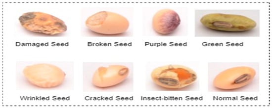
Figure 2. Sample of defective soybean seed datasets.

Experimental Set-Up

A NIKON D800 camera (Amravati, Maharashtra, India) is used to capture images of both good quality and defective soybean seeds. Two 11-watt lamps are placed on two sides of the table at a height of 12 inches from the table, and a camera at the same height is used to capture the pictures. The camera photographed each image of soybean samples placed on a white cloth at a distance of 12 inches and an angle ranging between 60° and 90° to the cloth. Pictures of each soybean seed are captured from all possible sides. Images are captured to depict soybean clusters containing 5 to 10 seeds, with a size of 7360 × 4912 pixels and a vertical and horizontal resolution of 300 dpi. Figure 3 shows the experimental setup to capture the soybean dataset.

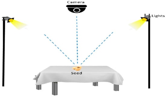
Figure 3. The experimental setup used to capture images for the soybean seed dataset.

3.2. Seed-Based Contour Detection (SCD) Algorithm

To enhance the quality of the soybean seed image, we propose a seed-based contour detection (SCD) algorithm that performs pre-processing operations on the seed. This algorithm is designed to accurately identify and isolate soybean seeds. It involves a series of steps to systematically process and analyze the visual data. Algorithm 1 represents the step-by-step execution of the SCD algorithm.

Algorithm 1. Seed-based contour detection (SCD) algorithm
Output Images	SCD Algorithm
Data:	Soybean Seed Dataset
Result:	Cropped Seed Image with Bounding Box around the seed in an image
SCD_A	← Input (Soybean dataset)  //Read the RGB image
SCD_B	← Extract_R(SCD_A)  //Extract the R component
SCD_C	← Apply_Median-Filter (SCD_B)  //Median filter using 3 × 3 window
SCD_D	← Apply_Gaussian-Filter (SCD_C)  //Perform Gaussian Blurring (sigma_x = 1, sigma_y = 1)
SCD_E	← Invert (SCD_D)  //Subtract from 255 (255-D)
SCD_F	← Binarize (SCD)  //Binarize (threshold = 128) (E > 128)
SCD_G	← Invert (SCD_F)  //Invert the image (1-F)
SCD_H	← Morphological_opertion (SCD_G)  //Perform Dilation & Erosion (7 × 7 window)
SCD_I	← Label_Regions (SCD_H)  //Label Regions
SCD_J	← Eliminate (SCD_I)  //Eliminate regions having pixels less than 1000
SCD_K	← Threshold (SCD_J)  //Threshold the image (J > 0) to obtain Mask (Necessary for multiple seeds)
SCD_L	← Apply_Bounding_Box_Algorithm (SCD_K)  //Apply Bounding Box Algorithm (BB)
SCD_M	← Locate_BB_Coordiates (SCD_L)  //Locate the extreme coordinates (Top left and bottom right) (for multiple Bounding boxes, top left of the top left box & bottom right of the bottom right box)
SCD_N	← Cropped (SCD_M) //Crop the seed image

The algorithm used RGB images from the dataset. Each image serves as the foundation for subsequent processing stages. Initially, it isolates the red component from the RGB image to enhance features specific to soybean seeds, as they often exhibit distinct characteristics in this color channel. In mathematical terms, for a given pixel at coordinates (x, y) in an RGB image represented as R_{(x, y)}, G_{(x, y)}, and B_{(x, y)} (denoting red, green, and blue color channels respectively), the extraction of the red component (R_{(x, y)}) can be expressed as:

$$R_{\left(x,y\right)}=Red Channel of Pixel at\left(x,y\right)$$

(1)

This operation essentially involves retaining the intensity values from the red channel while disregarding the green and blue components, resulting in an image where each pixel’s value represents only the red channel information. This can be symbolically represented as:

$$R_{\left(x,y\right)}=Intensity of Red Channel at \left(x,y\right)$$

(2)

To mitigate noise and irregularities within the image, a median filter using a 3 × 3 window is applied. This filtering process smoothens the image while preserving essential details. Applying a median filter with a 3 × 3 window to an image involves sorting the pixel values within the window and selecting the median value as the new value for the centre pixel. The process for a 3 × 3 median filter at a specific pixel location (x, y) can be represented as:

$$\begin{gathered} {I^{\prime }}_{new}\left(x,y\right)=median(I_{\left(x-1,y-1\right)},I_{\left(x,y-1\right)},I_{\left(x+1,y-1\right)}, \\ {I}_{\left(x-1, y\right)}, I_{\left(x, y\right)}, I_{\left(x+1, y\right)}, I_{\left(x-1, y+1\right)}, I_{\left(x, y+1\right)}, I_{\left(x+1, y+1\right)}) \end{gathered}$$

(3)

To reduce noise and blur the image slightly to prepare it for subsequent analysis, a Gaussian filter is used. At each pixel location (x, y) in the image, the filter operation computes a weighted average of the pixel values in the neighbourhood defined by the Gaussian kernel.

$${I^{\prime }}_{\left(x,y\right)}={\sum }_{i=-k}^k{\sum }_{j=-k}^k{G}_{\left(i,j\right)}.I_{\left(x-i,y-j\right)}$$

(4)

where ${I^{\prime }}_{\left(x,y\right)}$ is the new value of the pixel at position (x, y) after applying the Gaussian filter. $I_{\left(x,y\right)}$ represents the intensity value of the pixel at position (x, y) in the original image. $G_{\left(i,j\right)}$ is the Gaussian kernel value at position (i, j) within the filter. The sums are performed over the Gaussian kernel window, typically covering a region around the pixel (x, y), and $k$ determines the extent of the Gaussian kernel window, often related to the standard deviation.

By subtracting the filtered image from 255, the algorithm inverts the image. This inversion step sets the groundwork for binarization by applying a threshold to the inverted image. A threshold value of 128 is set to create a binary image, separating soybean seeds from the background. The resulting binarized image undergoes another inversion. This step prepares the image for morphological operations to further refine seed boundaries. To ensure the consistency of the background, the binary image is inverted. During this, tiny regions or holes within regions of interest became evident. Though these holes are potentially small, they hinder the accurate identification of seed boundaries and need addressing. Morphological operations play a vital role in preserving the shapes within images, especially in the context of binary images. In our process, four essential morphological operations are employed: dilation, closing, erosion, and opening. Morphological operations, specifically dilation followed by erosion, are employed to fill these holes. The concept is simple: dilation expands the white regions, thereby filling small black holes, and erosion then shrinks them back to preserve the general shape but without the holes. We utilized a 7 × 7 window, called a structuring element (SE), to ensure effective filling even for slightly larger holes. SE is a matrix or kernel used to modify the pixels of an image based on their neighbours. A significant point to mention is the choice of closing areas for post-dilation. By restricting the area to 50,000 pixels, we effectively maintained the integrity of our region of interest and ensured that there is no over-extension. Let us represent the input image and the structuring element SE is a small matrix or kernel that defines the neighbourhood used for morphological operations dilation, erosion, opening, and closing.

Dilation Operation (SE is a 7 × 7 window):

$$I_{dilated\left(x,y\right)}={max}_{\left(i,j\right)\in SE}{I}_{\left(x+i,y+j\right)}$$

(5)

Erosion Operation (SE is a 7 × 7 window):

$$I_{erosion\left(x,y\right)}={min}_{\left(i,j\right)\in SE}{I}_{\left(x+i,y+j\right)}$$

(6)

Opening Operation (Combination of Erosion followed by Dilation):

$$\begin{gathered} I_{opened\left(x,y\right)}=dilate\left(erode\right(I\left)\right) \\ {I}_{opened\left(x,y\right)}={max}_{\left(i,j\right)\in SE}{[min}_{\left(k,l\right)\in SE}{I}_{(x+k+i,y+l+j)}] \end{gathered}$$

(7)

Closing Operation (Combination of Dilation followed by Erosion):

$$\begin{gathered} I_{closed\left(x,y\right)}=erode\left(dilate\right(I\left)\right) \\ {I}_{closed\left(x,y\right)}={min}_{\left(i,j\right)\in SE}{[max}_{\left(k,l\right)\in SE}{I}_{(x+k+i,y+l+j)}] \end{gathered}$$

(8)

The Label Regions operation in image processing assigns unique labels or identifiers to different connected components or regions within an image. This process is performed using connected-component labelling algorithms. Connected pixels are identified by scanning the entire image and marking neighbouring pixels belonging to the same region. After an extensive experiment, we finalized that the threshold value was 1000 and eliminated small regions or components in an image that were smaller than a predefined threshold. This filtered out small, insignificant areas to refine and focus on larger, more substantial elements within the image. This process helps reduce noise or eliminate minor structures that might not be of interest to analysis or identification. Thresholding the image creates a mask essential for handling multiple seeds within an image. This process prepares for the next step of identifying bounding boxes. It gives a clear distinction between foreground and background elements, aiding in segmentation and feature extraction.

A bounding box algorithm is employed to precisely delineate the boundaries around individual soybean seeds. This crucial step provides a visual reference for accurate seed identification. The process involves finding the extreme coordinates (top-left and bottom-right corners) for each identified region. This bounding box delineates the spatial extent of the identified area, aiding in subsequent analysis or visualization. In the case of cracked, damaged, and insect-bitten seeds, regions were labelled more than once since the upper shell or coat of seeds was broken. Due to this, a single seed is differentiated into many small neighbouring regions or rectangles. In the case of a single region of interest, we cropped the region corresponding to the upper-left coordinate and bottom-right coordinate of the bounding box. We selected the top left and bottom right bounding boxes for multiple bounding boxes. Then, the top left coordinates of the former bounding box and the bottom right coordinates of the bottom right bounding box were used to extract the region of interest. As cracked, damaged, and insect-bitten seeds contained more than one bounding box, the remaining classes demonstrated a single bounding box, as shown in Figure 4. Using the coordinates obtained from the previous step, the algorithm crops individual seed images. These cropped images contain isolated soybean seeds, which are crucial for detailed analysis and further processing. Figure 5 represents the output of the SCD algorithm on a single insect-bitten seed image with three bounding boxes, and Figure 6 indicates the output of the SCD algorithm for multiple seeds and their bounding boxes. For our research work, we used single-seed images for further processing. The meticulous execution of each step within the seed contour detection algorithm ensures that noise is minimized, seed boundaries are accurately delineated, and the resulting images contain individual soybean seeds with clear bounding boxes, facilitating precise identification and analysis.

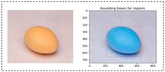
Figure 4. Output of SCD algorithm for single regions (1 bounding box) in a single seed.

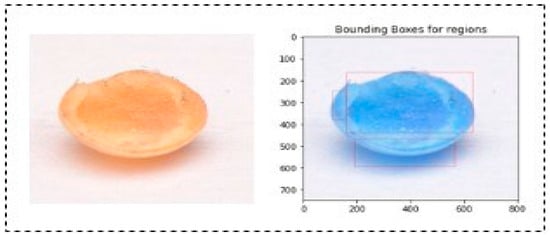
Figure 5. Output of SCD algorithm for multiple regions (3 bounding boxes) in a single seed.

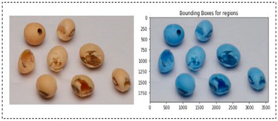
Figure 6. Output of SCD algorithm for multiple seeds and their bounding boxes.

3.3. Soybean Seed Defect Identification Network (SSDINet)

To identify defective soybean seeds, we designed the Soybean Seed Defect Identification Network (SSDINet). It is a lightweight and faster model that consists of convolutional layers (CONV), max-pooling layers, parallel executable depthwise convolution blocks, and squeeze-and-excitation blocks, followed by an average pooling layer and a flattening layer. For seed classification, four fully connected layers are utilized. Initially, features are extracted through the CONV layer, which consists of swish activation and batch normalization (BN). BN is used to address the issue of overfitting, followed by the max pooling layer, as shown in Figure 7. To reduce the parameters and channel-wise recalibration, depthwise separable convolution blocks (DSep-conv) and squeeze-and-excitation networks (SENet) are used simultaneously. Features extracted by DSep-conv and SENet are merged to effectively obtain good-quality spatial features. After the feature combination, an average pooling layer is applied, followed by a flattening layer. Last, four fully connected layers are employed for seed classification. The fully connected layers incorporate dense layers, ReLU activation, BN, and dropout. The last dense layer uses SoftMax for multi-class classification, transforming logits into probability distributions across classes. Algorithm 2 explains the steps in detail.

Algorithm 2. Soybean Seed Defect Identification Network (SSDINet)

Input: Enhanced Soybean seed dataset

Output: Classification of Soybean seed

Step 1: Z_CONV = Convolution (X, swish_activation, batch_normalization) //Feature Extraction through CONV Layer

Step 2: Z_MaxPool = MaxPooling(Z_CONV)  //Max Pooling Layer

Step 3: Z_DSep_conv = DepthwiseSeparableConv(Z_MaxPool) //Depthwise Separable Convolution Blocks (Deeps-conv) and Z_SENet = SqueezeAndExcitation(Z_MaxPool) //Squeeze-and-Excitation Networks (SENet)

Step 4: Z_Merged = Concatenate (Z_DSep_conv, Z_SENet) //Merge Features from DSep-conv and SENet

Step 5: Z_AvgPool = AveragePooling(Z_Merged)  //Average Pooling Layer

Step 6: Z_Flatten = Flatten(Z_AvgPool)  //Flatten Layer

Step 7: Z_Classif = FullyConnectedLayers(Z_Flatten)  //Four Fully Connected Layers

Step 8: Y = Softmax(Z_Classif)  //Softmax Activation for Multi-Class Classification

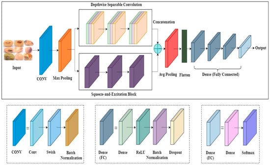
Figure 7. Architecture of Soybean Seed Defect Identification Network (SSDINet).

In SSDINet, DSep-conv and SENet play distinct but complementary roles in the feature extraction process. DSep-conv efficiently reduces the number of parameters while capturing spatial hierarchies in the input features. DSep-conv contains $K_d$ as depthwise filters, and $Z$ is a depthwise convolution result mentioned using Equation (9).

$$Z_{i,j,k}={\sum }_{m,n}{X}_{\left(i.s+m\right),\left(j.s+n\right),k}{K}_{d,m,n,k}$$

(9)

where $s$ is the stride, $i,j$ are spatial indices, $k$ is the channel index of the input feature map, $m,n$ is a convolution kernel index, and $K_{d,m,n,k}$ are the depthwise convolution filters. The depthwise convolution applies a separate convolution operation for each channel in the input feature map. The spatial dimensions are determined by the stride $s$. For pointwise convolution, $K_p$ is a pointwise filter and $Y$ as a final output feature map.

$$Y_{i,j,l}={\sum }_k{Z}_{i,j,k}{K}_{p,k,l}$$

(10)

where $l$ is an output channel index. The pointwise convolution combines the outputs from the depthwise convolution across channels. It applies a 1 × 1 convolution to mix and transform features. This results in a significant reduction in the number of parameters compared to traditional convolutions. Using DSep-conv, the model can maintain expressive power with fewer parameters, which is particularly beneficial for lightweight and faster models. It helps mitigate overfitting and improve computational efficiency. Figure 8 represents the structure of DSep-conv. Hence, the overall operation of DSep-conv can be represented as follows:

$$Y=Pointwise Conv(DepthwiseConv\left(X,K_d\right), K_p)$$

(11)

where $DepthwiseConv\left(X,K_d\right)$ represents the depthwise convolution and $Pointwise Conv(, K_p)$ represents the pointwise convolution. This makes SSDINet computationally more efficient and suitable for lightweight models.

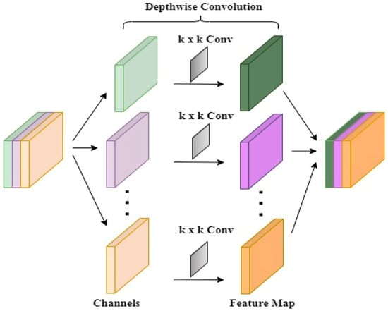
Figure 8. Depthwise separable convolution block (DSep-conv).

The task of SENet is to enhance channel-wise recalibration of feature responses, focusing on important information and suppressing less informative channels. SENet introduces an attention mechanism that adaptively recalibrates feature maps. Here, $X$ is an input feature map with dimensions $H\times W\times C$, where $H$ and $W$ are the spatial dimensions, and $C$ is the number of channels. It consists of a squeeze operation (global average pooling) to obtain channel-wise statistics, followed by an excitation operation (fully connected layers) to model interdependencies between channels shown in Figure 9.

$$Z_K=\frac{1}{H\times W}{\sum }_{i=1}^H{\sum }_{j=1}^W{X}_{i,j,k}\hspace{1em}\hspace{1em}\mathrm{Squeeze} \mathrm{operation}$$

(12)

$$S_k=\sigma (W_2.ReLU(W_1.Z_k\left)\right)\hspace{1em}\hspace{1em}\mathrm{Excitation} \mathrm{operation}$$

(13)

where $Z_k$ is the channel-wise statistic for the $k\mathrm{t}\mathrm{h}$ channel, also called a squeezed feature, $s_k$ is the excitation weight for the $k\mathrm{t}\mathrm{h}$ channel, $W_1,W_2$ are learnable parameters, $ReLU\left(\right)$ is a rectified linear unit activation function, and $\sigma \left(\right)$ is a sigmoid activation function. The output is multiplied element-wise with the input feature maps. SENet helps the model to focus on more relevant features by assigning different weights to different channels based on their importance. This adaptive recalibration improves the representational power of the network, contributing to better discrimination between different seed defects. The overall operation of the SENet can be summarized as follows:

$$Y=Scale(X, Excite(Squeeze\left(X\right)\left)\right)$$

(14)

where $Y$ represents the final feature map after adaptive recalibration through the squeeze-and-excitation mechanism.

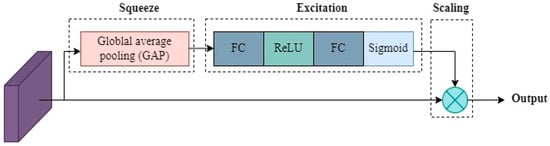
Figure 9. Squeeze-and-excitation networks (SENet).

4. Results

4.1. Evaluation Metrics

To assess the performance of SSDINet, confusion matrices play an essential role. True positive (TP), true negative (TN), false positive (FP), and false negative (FN) values in the confusion matrix are used to determine precision, recall, F1 score, and accuracy. A short description of these terms is summarized in Table 1.

Table 1. Mathematical equation and explanation of evaluation parameter [36].

Evaluation Metrics	Definition	Mathematical Equation
Precision (P)	Precision is the ratio of correctly predicted positive observations to the total predicted positives.	$P=\frac{TP}{TP + FP}$
Recall (R)	Recall is the ratio of correctly predicted positive observations to the total actual positives.	$R=\frac{TP}{TP + FN}$
F-Score (F-1)	F1 score is the harmonic mean of precision and recall.	$F1=\frac{2 \times Precion \times Recall}{Precion + Recall}$
Accuracy (Acc)	The ratio of correctly predicted observations (true positives and true negatives) to the total observations.	$Acc=\frac{TP + TN}{TP + TN + FP + FN}$

4.2. Dataset Distribution

To develop SSDINet, we used Python 3.7 as a programming language. The CPU requirement was met by a dual-core Intel Xeon processor, and GPU acceleration was achieved through NVIDIA T4 and P100, which is essential for efficient deep learning computations. Table 2 gives the details of the system requirements.

Table 2. Experimental requirement and software version.

Requirements	Details
Programming Language	Python 3.7
CPU	Dual-core Intel Xeon
GPU	NVIDIA T4 and P100
RAM	Up to 25 GB
Deep learning framework	Pytorch 1.11
Other packages	OpenCV 4.1, Seaborn 0.11, Pycocotools 2.0.6, tqdm 4.64 etc.

The dataset plays a crucial role in accurately identifying the class of soybean seed. It serves as the foundation for the model’s learning process, enabling it to recognize patterns and features unique to each seed class. We collected samples of 1000 soybean seeds, where we had 250 samples of good-quality seed, and the remaining were defective soybean samples which were further divided into 7 different classes as mentioned in detail in Table 3. To train the neural network efficiently after applying the SCD algorithm, we divided the dataset into three split ratios (80:20, 85:15, and 90:10) and observed their performances. From an experimental analysis, it was noted that an 80:20 ratio gave promising results, so for further investigation, we preferred an 80:20 ratio.

Table 3. Dataset distribution.

Soybean Seed Classes	Split Ratio
	80:20		85:15		90:10
	Training	Testing	Training	Testing	Training	Testing
Good seeds	200	50	212	38	225	25
Broken seeds	87	22	92	17	98	11
Cracked seeds	88	22	93	17	99	11
Damaged seeds	92	24	98	18	104	12
Insect-bitten seeds	90	23	96	17	101	12
Green seeds	76	20	81	15	86	10
Purple seeds	76	19	80	15	85	10
Wrinkled seeds	88	23	94	17	99	12

4.3. Performance of SSDINet

To train SSDINet on the soybean dataset, we used a categorical cross-entropy loss function, as the dataset is diversified. Categorical cross entropy was paired with the softmax activation function in the final output layer. Softmax transformed the raw model output into a probability distribution, and categorical cross-entropy gauged the dissimilarity between this distribution and the true distribution. The initial CNN layer utilized the swish activation function, while fully connected layers employed the ReLU activation function. Here, we used Adam optimizer, with a learning rate of 0.0001, weight decay of 0.0005, and 0.9 momentum, having batch size 4, and to train the network, 50 epochs were used. Figure 10 shows the gain in accuracy and decrease in loss of the SSDINet model during training and testing.

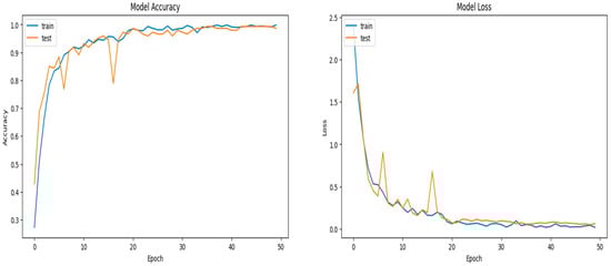
Figure 10. Graphical representation of epoch-wise accuracy and loss curve of the SSDINet model.

Table 4 represents the results of SSDINet for datasets 80:20, 85:15, and 90:10. Initially, the soybean dataset passed through the SCD algorithm, and then images were divided into the mentioned data split ratio and the network was trained. Notably, the data split ratio of 80:20 exhibited promising results after applying the SCD algorithm. While we also provided raw data images to SSDINet, there was a 3% gain in accuracy after applying the SCD algorithm. Hence, the proposed SCD algorithm helped to enhance the quality of soybean seed and also increased classification accuracy. Figure 11 indicates the graphical representation of SSDINet performance with and without SCD.

Table 4. The result of SSDINet with and without the SCD algorithm for various dataset split ratios.

Dataset Split Ratio	Model	Precision (%)	Recall (%)	F-1 Score (%)	Accuracy (%)
80:20	SSDINet without SCD algorithm	95.01	96.66	96.82	95.23
85:15		94.23	95.36	92.01	94.36
90:10		92.15	93.20	91.89	92.10
80:20	SSDINet with SCD algorithm	98.74	97.64	95.66	98.64
85:15		95.54	94.93	93.63	95.63
90:10		94.57	94.86	92.19	94.93

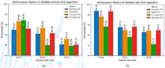
Figure 11. Performance of SSDINet (a) without SCD; (b) with SCD.

The classification performance of SSDINet to identify various soybean seed classes is summarized in Table 5 (values in brackets indicate the classes). The cracked seed, damaged seed, insect-bitten seed, green seed, purple seed, and wrinkled seed categories exhibited 100% accuracy, which was followed by the good seed and broken seed categories. Figure 12 shows the graphical representation of SSDINet output using the SCD algorithm for each class.

Table 5. Result of SSDINet with SCD algorithm for each class.

Soybean Seed Classes	Precision (%)	Recall (%)	F-1 Score (%)	Accuracy (%)
Broken seeds (0)	100	96	98	96
Cracked seeds (1)	92	100	96	100
Damaged seeds (2)	100	100	100	100
Insect-bitten seeds (3)	100	100	100	100
Green seeds (4)	100	100	100	100
Purple seeds (5)	93	100	97	100
Wrinkled seeds (6)	100	100	100	100
Good seeds (7)	100	98	99	97.7
Overall	98.74	97.64	98.66	98.64

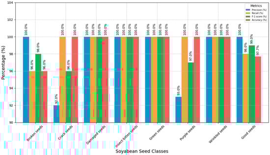
Figure 12. Graphical representation of SSDINet output using the SCD algorithm for each class.

4.4. Comparison of SSDINet with Other Models

In this section, the proposed SSDINet model is compared with the traditional classification method of machine learning (ML) and essential deep learning (DL) model, i.e., CNN. ML techniques include logistic regression (LR), support vector machine (SVM), and k-nearest neighbour (KNN), while DL uses CNN+ dense layer. Table 6 shows the comparison of SSDINet with traditional models. Among the traditional ML techniques, SVM emerges as the top performer with the highest accuracy of 91.89%. LR and KNN trail behind, where LR exhibits an accuracy of 81.98% and KNN achieves 79.28%. In contrast, a DL-based CNN model outperforms traditional ML methods with a substantially higher precision of 94.20%, recall of 92.67%, F1 score of 93.50%, and accuracy of 93.69%. The proposed SSDINet surpasses the other models and attains the highest precision of 98.74%, recall of 97.64%, F1 score of 98.66%, and accuracy of 98.64%. These results underscore the superiority of DL-based approaches, particularly SSDINet, in accurately classifying soybean seeds based on their defects. This signifies their potential for enhancing quality control processes in the soybean industry. Figure 13 indicates the confusion metrics of conventional ML, DL, and SSDINet models.

Table 6. Comparison of the proposed model with other traditional models.

Models	Precision (%)	Recall (%)	F-1 Score (%)	Accuracy (%)
KNN	86.43	78.58	78.54	79.28
LR	85.96	81.78	79.37	81.98
SVM	92.93	90.79	91.85	91.89
CNN	94.20	92.67	93.50	93.69
SSDINet (our)	98.74	97.64	98.66	98.64

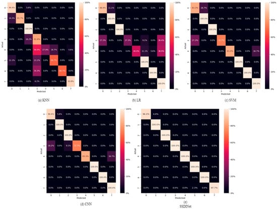
Figure 13. Confusion matrices of traditional ML, DL, and SSDINet models.

5. Discussion

The proposed faster and lightweight SSDINet model is compared with the state-of-the-art models SNet and SoyNet in terms of accuracy, size, classification time, precision, recall, and F1 score, as shown in Table 7. In terms of accuracy, SSDINet achieves 98.64%, which surpasses both SNet and SoyNet. Notably, SSDINet accomplishes a high level of performance with a smaller model size (1.15 M Params) compared to SNet and SoyNet, demonstrating efficiency in resource utilization. Furthermore, SSDINet demonstrates competitive inference times of 4.70 ms, comparable to SoyNet and significantly faster than SNet. This comprehensive analysis underscores SSDINet’s effectiveness, efficiency, and superiority over the other models in the context of soybean seed classification.

Table 7. Comparison with state-of-the-art approaches.

Model	Precision (%)	Recall (%)	F-1 Score (%)	Accuracy (%)	Size (Params)	Time
SNet [32]	97.0	94.0	95.5	96.2	1.29 M	9.67 ms
SoyNet [37]	96.69	96.71	96.69	95.63	7.26 M	4.92 ms
SSDINet (Our)	98.74	98.64	98.64	98.64	1.15 M	4.70 ms

6. Conclusions

This article introduces a lightweight soybean seed defect identification network (SSDINet) designed to quickly and accurately differentiate between good and defective soybean seeds. Initially, we developed a soybean seed dataset with 8 classes comprising 7 defective categories and 1 good quality category and consisting of 1000 samples. A seed contour detection (SCD) algorithm is proposed to enhance the quality of the seed. The proposed SCD algorithm facilitates segmentation before passing the dataset to SSDINet. The SSDINet classification network comprises a convolutional neural network, depthwise convolution blocks, and squeeze-and-excitation blocks. This choice of the proposed architecture enhances the network’s efficiency, speed, and accuracy compared to conventional ML, CNN and existing state-of-the-art approaches. Experimental results demonstrate that SSDINet achieves the highest accuracy at 98.64% with a modest parameter size of 1.15 million, completing the classification task in 4.70 milliseconds. These results surpass the performance of current state-of-the-art models, confirming the effectiveness of SSDINet in the rapid and accurate identification of soybean seed defects. The proposed architecture ensures a systematic and accurate identification of soybean seed quality through collaborative efforts and advanced image processing techniques. In the future, we plan to develop a real-time system for soybean identification, aiming to bridge the gap between research innovation and practical implementation. This approach seeks to maximize the impact of our work in real-world applications within the soybean industry.

References

- Medic, J.; Atkinson, C.; Hurburgh, C.R. Current knowledge in soybean composition. JAOCS J. Am. Oil Chem. Soc. 2014, 91, 363–384. [Google Scholar] [CrossRef]
- Carther, K.F.I.; Ketehouli, T.; Ye, N.; Yang, Y.-H.; Wang, N.; Dong, Y.-Y.; Yao, N.; Liu, X.-M.; Liu, W.-C.; Li, X.-W.; et al. Comprehensive Genomic Analysis and Expression Profiling of Diacylglycerol Kinase (DGK) Gene Family in Soybean (Glycine max) under Abiotic Stresses. Int. J. Mol. Sci. 2019, 20, 1361. [Google Scholar] [CrossRef]
- Chen, K.I.; Erh, M.H.; Su, N.W.; Liu, W.H.; Chou, C.C.; Cheng, K.C. Soyfoods and soybean products: From traditional use to modern applications. Appl. Microbiol. Biotechnol. 2012, 96, 9–22. [Google Scholar] [CrossRef]
- Wu, Y.M.; Guan, R.X.; Liu, Z.X.; Li, R.Z.; Chang, R.Z.; Qiu, L.J. Synthesis and Degradation of the Major Allergens in Developing and Germinating Soybean Seed. J. Integr. Plant Biol. 2012, 54, 4–14. [Google Scholar] [CrossRef]
- Radchuk, V.; Physical, L.B. Metabolic and developmental functions of the seed coat. Front. Plant Sci. 2014, 5, 510. [Google Scholar]
- Boulila, W.; Alzahem, A.; Koubaa, A.; Benjdira, B.; Ammar, A. Early detection of red palm weevil infestations using deep learning classification of acoustic signals. Comput. Electron. Agric. 2023, 212, 108154. [Google Scholar] [CrossRef]
- Yang, S.; Zheng, L.; He, P.; Wu, T.; Sun, S.; Wang, M. High-throughput soybean seeds phenotyping with convolutional neural networks and transfer learning. Plant Methods 2021, 17, 50. [Google Scholar] [CrossRef] [PubMed]
- Alzahem, A.; Boulila, W.; Koubaa, A.; Khan, Z.; Alturki, I. Improving satellite image classification accuracy using GAN-based data augmentation and vision transformers. Earth Sci. Inform. 2023, 16, 4169–4186. [Google Scholar] [CrossRef]
- Khan, A.R.; Javed, R.; Sadad, T.; Bahaj, S.A.; Sampedro, G.A.; Abisado, M. Early pigment spot segmentation and classification from iris cellular image analysis with explainable deep learning and multiclass support vector machine. Biochem. Cell Biol. 2023. [Google Scholar] [CrossRef]
- Mahmood, T.; Rehman, A.; Saba, T.; Nadeem, L.; Bahaj, S.A. Recent advancements and future prospects in active deep learning for medical image segmentation and classification. IEEE Access 2023, 11, 113623–113652. [Google Scholar] [CrossRef]
- Varone, G.; Boulila, W.; Driss, M.; Kumari, S.; Khan, M.K.; Gadekallu, T.G.; Hussain, A. Finger pinching and imagination classification: A fusion of CNN architectures for IoMT-enabled BCI applications. Inf. Fusion 2024, 101, 102006. [Google Scholar] [CrossRef]
- Bashir, M.H.; Ahmad, M.; Rizvi, D.R.; El-Latif, A.A. Efficient CNN-based disaster events classification using UAV-aided images for emergency response application. Neural Comput. Appl. 2024. [Google Scholar] [CrossRef]
- Boulila, W.; Ghandorh, H.; Masood, S.; Alzahem, A.; Koubaa, A.; Ahmed, F.; Khan, Z.; Ahmad, J. A Transformer-based Approach Empowered by a Self-Attention Technique for Semantic Segmentation in Remote Sensing. Heliyon 2024, 10, e29396. [Google Scholar] [CrossRef]
- Wang, L.; Liu, J.; Zhang, J.; Wang, J.; Fan, X. Corn Seed Defect Detection Based on Watershed Algorithm and Two-Pathway Convolutional Neural Networks. Front. Plant Sci. 2022, 13, 730190. [Google Scholar] [CrossRef]
- Sun, J.; Zhang, Y.; Zhu, X.; Zhang, Y.D. Enhanced individual characteristics normalized lightweight rice-VGG16 method for rice seed defect recognition. Multimed. Tools Appl. 2023, 82, 3953–3972. [Google Scholar] [CrossRef]
- Boniecki, P.; Sujak, A.; Pilarska, A.A.; Piekarska-Boniecka, H.; Wawrzyniak, A.; Raba, B. Dimension Reduction of Digital Image Descriptors in Neural Identification of Damaged Malting Barley Grains. Sensors 2022, 22, 6578. [Google Scholar] [CrossRef] [PubMed]
- Fazel-Niari, Z.; Afkari-Sayyah, A.H.; Abbaspour-Gilandeh, Y.; Herrera-Miranda, I.; Hernández-Hernández, J.L.; Hernández-Hernández, M. Quality assessment of components of wheat seed using different classifications models. Appl. Sci. 2022, 12, 4133. [Google Scholar] [CrossRef]
- Du, X.; Si, L.; Li, P.; Yun, Z. A method for detecting the quality of cotton seeds based on an improved ResNet50 model. PLoS ONE 2023, 18, e0273057. [Google Scholar] [CrossRef]
- Barrio-Conde, M.; Zanella, M.A.; Aguiar-Perez, J.M.; Ruiz-Gonzalez, R.; Gomez-Gil, J. A Deep Learning Image System for Classifying High Oleic Sunflower Seed Varieties. Sensors 2023, 23, 2471. [Google Scholar] [CrossRef]
- Xiao, Z.; Yuan, F. Sorting and Identification Method of Camellia Seeds Based on Deep Learning. In Proceedings of the 2021 40th Chinese Control Conference (CCC), Shanghai, China, 26–28 July 2021; Available online: https://ieeexplore.ieee.org/abstract/document/9550450/ (accessed on 7 October 2023).
- Zhang, L.; Wang, D.; Liu, J.; An, D. Vis-NIR hyperspectral imaging combined with incremental learning for open world maize seed varieties identification. Comput. Electron. Agric. 2022, 199, 107153. [Google Scholar] [CrossRef]
- Liu, Q.; Wang, Z.; Long, Y.; Zhang, C.; Fan, S.; Huang, W. Variety classification of coated maize seeds based on Raman hyperspectral imaging. Spectrochim. Acta Part A Mol. Biomol. Spectrosc. 2022, 270, 120772. [Google Scholar] [CrossRef]
- Huang, S.; Fan, X.; Sun, L.; Shen, Y.; Suo, X. Research on classification method of maize seed defect based on machine vision. J. Sens. 2019, 2019, 2716975. [Google Scholar] [CrossRef]
- Xu, P.; Tan, Q.; Zhang, Y.; Zha, X.; Yang, S.; Yang, R. Research on maize seed classification and recognition based on machine vision and deep learning. Agriculture 2022, 12, 232. [Google Scholar] [CrossRef]
- Zhou, Q.; Huang, W.; Fan, S.; Zhao, F.; Liang, D.; Tian, X. Non-destructive discrimination of the variety of sweet maize seeds based on hyperspectral image coupled with wavelength selection algorithm. Infrared Phys. Technol. 2020, 109, 103418. [Google Scholar] [CrossRef]
- Gulzar, Y.; Hamid, Y.; Soomro, A.B.; Alwan, A.A.; Journaux, L. A convolution neural network-based seed classification system. Symmetry 2020, 12, 2018. [Google Scholar] [CrossRef]
- Zhao, L.; Haque, S.R.; Wang, R. Automated seed identification with computer vision: Challenges and opportunities. Seed Sci. Technol. 2022, 50, 75–102. [Google Scholar] [CrossRef]
- Jin, B.; Zhang, C.; Jia, L.; Tang, Q.; Gao, L.; Zhao, G.; Qi, H. Identification of Rice Seed Varieties Based on Near-Infrared Hyperspectral Imaging Technology Combined with Deep Learning. ACS Omega 2022, 7, 4735–4749. [Google Scholar] [CrossRef] [PubMed]
- Zhu, L.; Spachos, P.; Pensini, E.; Plataniotis, K.N. Deep learning and machine vision for food processing: A survey. Curr. Res. Food Sci. 2021, 4, 233–249. [Google Scholar] [CrossRef]
- Sable, A.V.; Singh, P.; Singh, J.; Hedabou, M. A Survey on Soybean Seed Varieties and Defects Identification Using Image Processing. In ACI@ ISIC; CEUR Workshop Proceedings: Milan, Italy, 2021; Volume 3283, pp. 61–69. [Google Scholar]
- Hu, X.; Yang, L.; Zhang, Z. Non-destructive identification of single hard seed via multispectral imaging analysis in six legume species. Plant Methods 2020, 16, 116. [Google Scholar] [CrossRef]
- Huang, Z.; Wang, R.; Cao, Y.; Zheng, S.; Teng, Y.; Wang, F.; Wang, L.; Du, J. Deep learning based soybean seed classification. Comput. Electron. Agric. 2022, 202, 107393. [Google Scholar] [CrossRef]
- Lin, W.; Lin, Y.; Phys, J.; Wang, Y.; Xu, S.; Li, G. Soybean image segmentation based on multi-scale Retinex with color restoration. J. Phys. Conf. Ser. 2022, 2284, 12010. [Google Scholar] [CrossRef]
- Liu, H.; Qu, F.; Yang, Y.; Li, W.; Hao, Z. Soybean Variety Identification Based on Improved ResNet18 Hyperspectral Image. J. Phys. Conf. Ser. 2022, 2284, 012017. [Google Scholar] [CrossRef]
- Baek, J.; Lee, E.; Kim, N.; Kim, S.L.; Choi, I.; Ji, H.; Chung, Y.S.; Choi, M.-S.; Moon, J.-K.; Kim, K.-H. High throughput phenotyping for various traits on soybean seeds using image analysis. Sensors 2019, 20, 248. [Google Scholar] [CrossRef] [PubMed]
- Maxwell, A.E.; Warner, T.A.; Guillén, L.A. Accuracy Assessment in Convolutional Neural Network-Based Deep Learning Remote Sensing Studies—Part 1: Literature Review. Remote Sens. 2021, 13, 2450. [Google Scholar] [CrossRef]
- Lin, W.; Shu, L.; Zhong, W.; Lu, W.; Ma, D.; Meng, Y. Online classification of soybean seeds based on deep learning. Eng. Appl. Artif. Intell. 2023, 123, 106434. [Google Scholar] [CrossRef]
Disclaimer/Publisher’s Note: The statements, opinions and data contained in all publications are solely those of the individual author(s) and contributor(s) and not of MDPI and/or the editor(s). MDPI and/or the editor(s) disclaim responsibility for any injury to people or property resulting from any ideas, methods, instructions or products referred to in the content. |
© 2024 by the authors. Licensee MDPI, Basel, Switzerland. This article is an open access article distributed under the terms and conditions of the Creative Commons Attribution (CC BY) license (https://creativecommons.org/licenses/by/4.0/).