Article

Predrought and Its Persistence Determined the Phenological Changes of Stipa krylovii in Inner Mongolia

1
Department of Atmospheric and Oceanic Sciences & Institute of Atmospheric Sciences, Fudan University, Shanghai 200438, China
2
State Key Laboratory of Severe Weather, Chinese Academy of Meteorological Sciences, Beijing 100081, China
3
Joint Eco-Meteorological Laboratory of Chinese Academy of Meteorological Sciences, Zhengzhou University, Zhengzhou 450001, China
4
College of Resources and Environmental Sciences, China Agricultural University, Beijing 100193, China
*
Author to whom correspondence should be addressed.
Agronomy 2023, 13(5), 1345; https://doi.org/10.3390/agronomy13051345
Submission received: 14 April 2023 / Revised: 4 May 2023 / Accepted: 9 May 2023 / Published: 11 May 2023

Abstract

:
Clarifying the response of plant phenology to drought duration is helpful for accurately interpreting and predicting carbon sinks in ecosystems. Based on the response of different phenological periods of the dominant species Stipa krylovii to monthly, seasonal, and semiannual time scale drought in the typical steppe of Inner Mongolia from 1983 to 2018, the results revealed that (1) the start of the growing season (SOS) was characterized by an advance–delay–advance pattern, and the heading stage (HOS), flowering stage (FOS), and end of the growing season (EOS) all showed consistent advanced trends, which provided additional insight into the conclusions of previous studies that found the SOS was advanced in arid and semiarid regions. (2) The response mechanism of the SOS to the timing of drought was not consistent. Among the response mechanism, the SOS was delayed because of the January–February drought at different time scales but advanced because of the April drought at different time scales. The HOS/FOS was delayed by the June–July drought at different time scales, and the EOS was advanced by the August–September drought at different time scales. (3) More importantly, the SOS, HOS, FOS, and EOS were affected by predrought and its persistence, and the effects were greater the closer to the phenological periods that drought occurred. (4) At the monthly scale, droughts in January, June, and August were the critical drought periods affecting the SOS, HOS/FOS, and EOS, while seasonal and semiannual scale droughts in February, June–July, and September were the critical periods affecting the SOS, HOS/FOS, and EOS. The results of this study enrich our understanding of how drought at different time scales affects different phenological periods, providing a basis for improving plant phenological models.

1. Introduction

Plant phenology refers to the timing of periodic biological events in nature that are driven by climatic and environmental factors and recur in an annual cycle; it is a sensitive indicator of the response of ecosystems to climate change [1,2] and plays a fundamental role in regulating global carbon, water and nutrient cycles [3]. The intensity and frequency of droughts have increased dramatically in the context of global warming [4,5,6], with more severe impacts on plant phenology [3,7]. Research has shown that severe drought and heavy rainfall events can cause the same degree of plant phenology change as 10 years of warming [8]. Therefore, identifying the effects of drought on plant phenology is of great importance in global change research [7,9] and has become a research hotspot [1,10].
Drought causes changes in vegetation phenology as well as in productivity by altering vegetation vitality [11,12,13,14,15]. There are inconsistent conclusions about the effects of drought on phenology. Studies have shown that drought leads to earlier spring and autumn plant phenology in the Northern Hemisphere at mid and high latitudes [10,16]. However, it has been suggested that drought has caused a delay in spring phenology and earlier autumn phenology in the Canadian Prairies [17]; it has induced delayed spring phenology in grassland ecosystems and, conversely, has brought about advanced spring phenology within forest ecosystems across the Northeast China Transect [18] and had induced delayed spring phenology and an advanced trend in autumn phenology in Southwest China [19]. This suggests that understanding the effects of drought on plant phenology may provide important insights into the future response of plant phenology to climate change [16].
Studies have explored the effects of drought on vegetation phenology in ecosystems mainly on a regional or global scale [10,11,20] and have mostly used remote sensing data as the basis for statistical methods to invert plant phenological periods and thus identify the response of plant phenology to drought at the community or landscape scale [21]. Therefore, the results of analyses of phenological responses to drought have been inconsistent. In addition, drought is characterized by multiple time scales, and the effects of drought at different time scales need to be considered when assessing the response of plant phenology to drought. Generally, the indices used to quantify the magnitude and duration of drought include the Palmer drought severity index (PDSI), the standardized precipitation index (SPI), and the standardized precipitation evapotranspiration index (SPEI) [12,20,22]. The SPEI, which takes into account the impact of potential evapotranspiration (PET), explains the possible effects of temperature changes and extreme temperatures [20] and is more suitable for describing drought conditions under climate warming [23]. The SPEI has been widely used to analyze the impact of drought on vegetation dynamics [21,24,25,26].
The changes of the phenological periods are a key mechanism for ecosystem responses to drought yet remain unknown at different time scales, which limit the understanding and quantitative modeling of plant phenological mechanisms of drought response and affect the accurate assessment of carbon sequestration in terrestrial ecosystems [27]. However, the phenological period's response to drought is complex and has not yet been thoroughly investigated. There is no consensus on whether the start of the growing season (SOS) is earlier or later in the context of drought. In addition to the SOS, the heading stage (HOS), flowering stage (FOS), and end of the growing season (EOS) response to drought should also be paid more attention. The SOS of grassland in the semi-arid regions of northern China could be delayed by drought in previous months [14]. Hence, this study focuses on the phenology difference between the drought and normal periods and attempts to explore the effects of drought on the different phenological periods at different time scales. The grassland ecosystem of Inner Mongolia is highly sensitive to drought events caused by climate warming, especially in arid and semiarid areas with precipitation of 200–300 mm [18]. Based on the different phenological periods of S. krylovii and the corresponding meteorological data in the typical steppe of Inner Mongolia during the period from 1983 to 2018. This study aims to (1) elucidate the response characteristics of different phenological periods of S. krylovii to drought at different time scales and (2) reveal the critical periods of different phenological periods in response to drought at different time scales.

2. Materials and Methods

2.1. Study Area and Data

Xilinhot (116°19′ E, 44°08′ N) in the central part of the Xilingol League, which is a typical temperate semiarid continental climate zone, was used as the study area. From 1981 to 2018, the mean annual temperature and annual precipitation were 3.2 °C and 278.5 mm, respectively, and the annual cumulative sunlight hours were 2960.7 h.
In this study, the phenology dataset of the typical steppe dominant species S. krylovii included the SOS, HOS, FOS, and EOS from 1983 to 2018. These data were obtained at the natural pasture observation site of the Xilinhot National Climate Observatory, Inner Mongolia, China Meteorological Administration. In addition, the meteorological dataset includes the daily mean air temperature (°C), maximum air temperature (°C), minimum air temperature (°C), precipitation (mm), sunlight hours (h), relative humidity (%), and mean wind speed (m/s) in Xilinhot from 1981 to 2018. The fenced area of the observation field was 100 m × 100 m and was divided into four plots of 50 m × 50 m, with each plot divided into four replicates for observation. Phenological periods, which were recorded by local professional observers in accordance with standard observation protocols [28], were observed every 2 d. Ten plants with robust growth and complete life history for three consecutive years were selected for observation [29].

2.2. Methods

The phenological periods were converted into Julian days (with 1 January as the first day of each year) for statistical analysis. The trend analysis method and moving average method were used to analyze the changing trend of different phenological periods of S. krylovii from 1983 to 2018. Partial least squares (PLS) regression was used to analyze the critical periods of phenological response to drought at different time scales.

2.2.1. Standardized Precipitation Evapotranspiration Index

The standardized precipitation evapotranspiration index (SPEI), based on the input data of monthly mean air temperature and precipitation, standardizes the difference between monthly precipitation and potential evapotranspiration with different time scales [23]. The different time scales of the SPEI are used to indicate the cumulative climate water balance over the preceding few months. A larger SPEI corresponds to a humid climate, while a smaller SPEI corresponds to a dry climate.
First, monthly potential evapotranspiration (PET) based on the Thornthwaite method was calculated as follows:
P E T = 16 K ( 10 T i I ) m
where Ti is the monthly mean temperature (°C), K is the correction coefficient calculated according to latitude, I is the annual total heating index, and m is the coefficient determined by I.
Second, the monthly difference in precipitation and potential evapotranspiration (PET) was calculated as follows:
D i = P i P E T i
where Pi is the monthly precipitation (mm) and PETi is the monthly potential evapotranspiration (mm/month).
Third, the sequences of climatic water equilibrium accumulation at different time scales were established:
D n k = i = 0 k 1 ( P n i P E T n i ) , n k
where k is the time scale and n is the number of calculations.
Fourth, the data sequence was constructed by fitting the log-logistic probability density function (f(x)) and the cumulative probability density (F(x)) of a given time scale:
f ( x ) = β α ( x γ α ) β 1 [ 1 + ( x γ α ) β ] 2
F ( x ) = [ 1 + ( α x γ ) β ] 1
where α, β, and γ are the scale coefficient, shape coefficient, and origin parameter, respectively.
Finally, the corresponding SPEI variation series was obtained by transforming the standard normal distribution of F(x):
When P ≤ 0.5:
S P E I = ω c 0 + c 1 ω + c 2 ω 2 1 + d 1 ω + d 2 ω 2 + d 3 ω 3
ω = 2 ln ( P )
When P > 0.5:
S P E I = ω c 0 + c 1 ω + c 2 ω 2 1 + d 1 ω + d 2 ω 2 + d 3 ω 3
where P is the probability of exceeding the determined moisture profit and loss, and c0 = 2.515517, c1 = 0.802853, c2 = 0.010328, d1 = 1.432788, d2 = 0.189269, d3 = 0.001308. In this way, the characteristics of drought on a monthly scale (SPEI-1), seasonal scale (SPEI-3), and semiannual scale (SPEI-6) could be calculated from 1983 to 2018.

2.2.2. Partial Least Squares Regression

Partial least squares regression (PLS) is widely used in the response of plant phenology to climate change [30,31]. Variable importance in projection (VIP) and the standardized model coefficient (MC) are the two main output indices of PLS [32,33,34]. The VIP values are used to determine the explanatory ability of independent variables on the dependent variable; the higher the VIP is, the more significant the explanatory power of the independent variable on the dependent variable is [35]. A VIP ≥ 1 indicates significant explanatory power, while 0.8 ≤ VIP < 1 indicates general explanatory power, and a VIP < 0.8 indicates essentially no explanatory power. The MC quantifies the strength and direction of the influence of the independent variable on the dependent variable.

3. Results

3.1. Phenological Variation Characteristics of S. krylovii

The average SOS, HOS, FOS, and EOS of S. krylovii appeared in mid-late April, late July, mid-August, and early October from 1983 to 2018, respectively. During the study period, the SOS was delayed at a rate of 4.4 d/10a. To reduce the influence of random error, the 3a moving average method was used to process the phenological time series. We highlighted that the changing direction of SOS occurred at different time stages. Before 1995, the SOS showed an advanced trend and then a delayed trend from 1995 to 2010; after 2010, it showed an advanced trend (Figure 1a). The HOS and FOS showed a significant advancing trend (Figure 1b,c), and the rates were −5.5 d/10a and −10.1 d/10a, respectively. In addition, the advancing trend of HOS after 2000 was significantly lower than that before 2000, while the advancing trend of FOS after 2000 was more obvious. The EOS showed an insignificant advancing trend, with the largest variation approximately in 2001 (Figure 1d). In general, the SOS showed an advance–delay–advance pattern during the study period. The HOS, FOS, and EOS showed an advanced trend, among which the advance amplitude of FOS was the largest, indicating that the vegetative growth period was shortened and the reproductive growth period was prolonged.

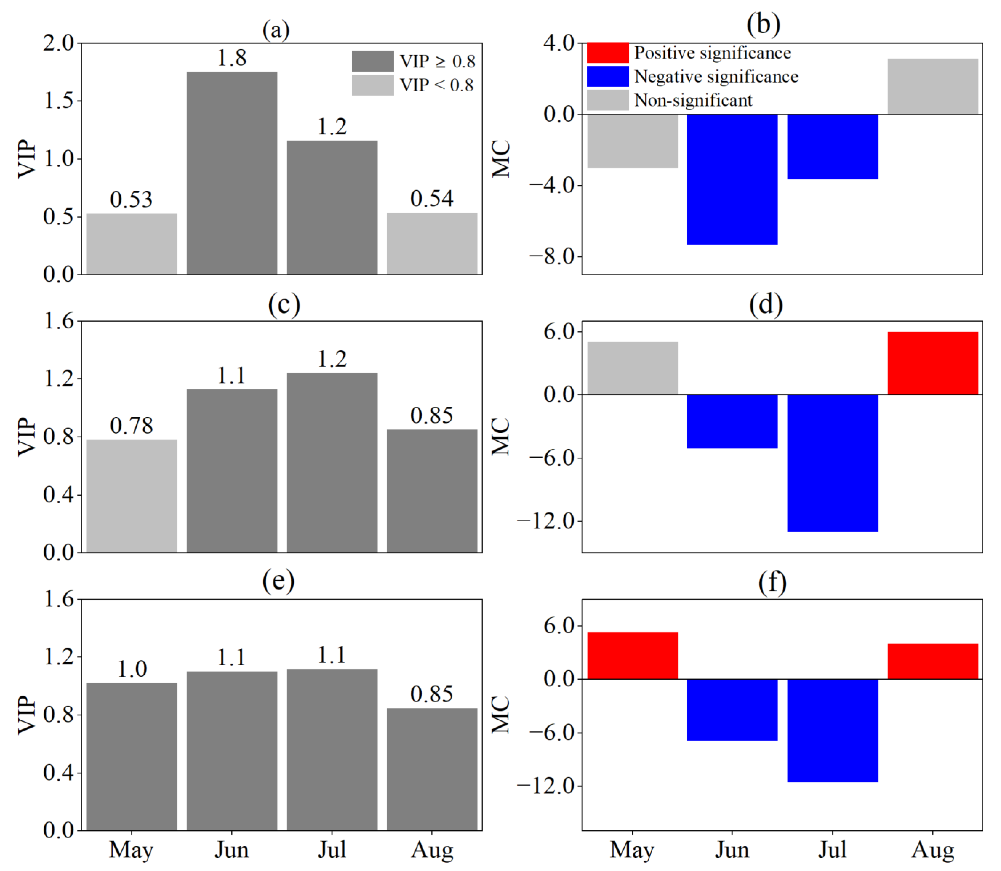
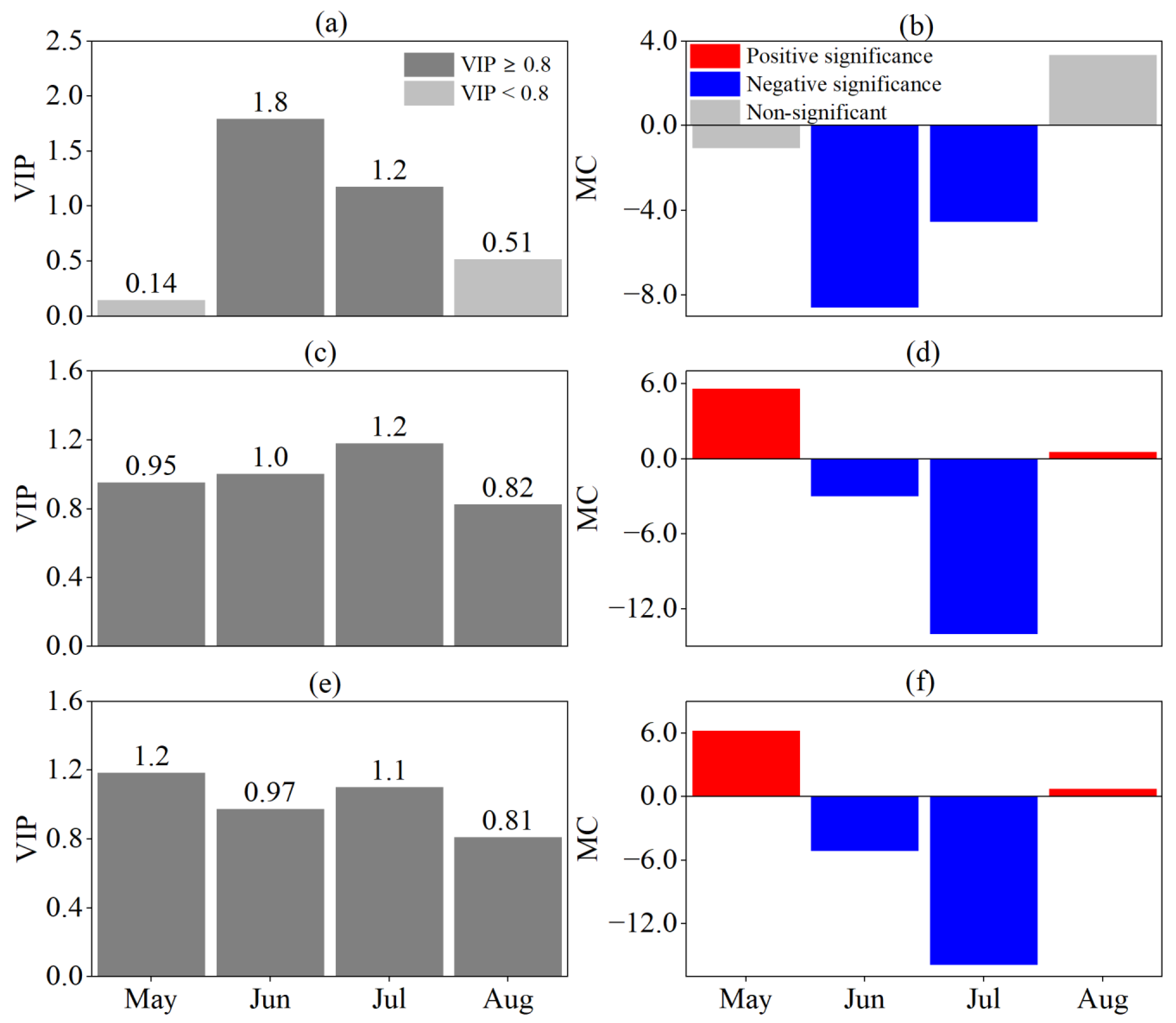
3.2. Response of Phenological Periods to Drought at Different Time Scales

According to the drought grade of the SPEI, conditions can be divided into three categories: drought (SPEI < –1.0), normal (–1.0 ≤ SPEI < 0.5), and moist (SPEI ≥ 0.5). The SOS was delayed by the January–February drought at different time scales, while it was advanced by the April drought at different time scales (Figure 2). Among the time scales, for the monthly scale, the difference between the dry climate and normal climate in January was significant for the SOS (p < 0.05), while for the seasonal scale, the difference between the dry climate and normal climate in February and April was significant for the SOS (p < 0.05, p < 0.01), respectively. Meanwhile, for the semiannual scale, the difference between the dry climate and normal climate in January and February was significant for the SOS (p < 0.05 and p < 0.01, respectively). Drought at different time scales delayed the HOS and FOS (Figure 3 and Figure 4). Among the time scales, the difference between the dry climate and normal climate in July was significant for the HOS (p < 0.01). On the monthly scale, the difference between the dry climate and the normal climate in June was significant for the FOS (p < 0.05). For the seasonal scale, the difference between the dry climate and the normal climate in August was significant for the FOS (p < 0.05). Drought at different time scales resulted in an earlier EOS (Figure 5). Among the scales, at the monthly scale, the difference between the dry climate and normal climate in August was significant for the EOS (p < 0.05).
Overall, the SOS was delayed by the January–February drought but advanced by the April drought at different time scales. The HOS and FOS were delayed by predrought, and the EOS was advanced by predrought.

3.3. Drought Time Scale Affecting the Phenological Period

The SOS response to the SPEI at different time scales was consistent (Figure 6). There was a significant negative correlation between the SPEI and the SOS in January and February on a monthly scale (VIP ≥ 0.8, MC < 0) and between the SPEI and the SOS in January, February, and March on a seasonal scale (VIP ≥ 0.8, MC < 0), and there was a significant negative correlation between the SPEI and the SOS in February on a semiannual scale (VIP ≥ 0.8, MC < 0). At the same time, the SPEI in April was significantly and positively correlated with the SOS (VIP ≥ 0.8, MC > 0). This indicated that the SOS was influenced by predrought and its persistence and that the effect of persistent drought was greater the closer to the SOS.
The HOS and FOS response to the SPEI at different time scales were consistent (Figure 7 and Figure 8). In June and July, the HOS and FOS were negatively correlated with the SPEI at different time scales (VIP ≥ 0.8, MC < 0). The most significant effects of drought on the HOS and FOS were observed in June on a monthly scale and in July on seasonal and semiannual scales. The VIP values indicated that the HOS and FOS were influenced by the predrought and its persistence and that the effect of persistent drought was greater the closer to the HOS and FOS it occurred.
The effect of the SPEI at different time scales on the EOS was also generally consistent (Figure 9). On the monthly scale, August SPEI was significantly positively correlated with the EOS (VIP ≥ 0.8, MC > 0) with the highest VIP value, and at the seasonal scale, September SPEI was significantly positively correlated with the EOS (VIP ≥ 0.8, MC > 0). On the semiannual scale, September SPEI was positively correlated with the EOS. This suggested that the EOS was influenced by the predrought and its persistence and that the effect of persistent drought was greater the closer to the EOS it occurred.
PLS analysis showed that at the monthly scale, the critical periods for the response of the SOS, HOS/FOS, and EOS to drought were January, June, and August, and at the seasonal or semiannual scale, the critical periods were February, June–July, and September, respectively.

4. Discussion

Climate warming usually increases water stress and thus delays plant growth in arid and semiarid regions [36,37]. A large number of studies have shown that the advances SOS and delays EOS [9,38]. Our study showed that for S. krylovii in the typical steppe of Inner Mongolia, the SOS was delayed and that the HOS, FOS, and EOS were advanced, which was consistent with the findings concerning phenological changes based on remote sensing inversion in central and eastern Inner Mongolia [14]. In addition, other species-level studies have shown that the SOS of S. krylovii, L. chinensis, A. frigida, and C. sphaeroides were significantly delayed in typical steppe [39,40,41,42]. Although a delayed SOS was observed during the study period, the direction of its variation at different periods was not consistent. In other words, the SOS showed a dynamic feature of advance–delay–advance during 1983–2018, which provided additional insight into the conclusions of previous research.
Water availability is a limiting factor for plant growth in arid and semiarid regions [43] and is an important factor in regulating plant phenological responses to warming [37]. Moreover, predrought has been shown to play a key role in determining the direction of the SOS [15]. Studies have shown that predrought delays the SOS of herbaceous plants [14,44,45]. The present study showed that the phenological period was closely related to the degree of drought at different time scales and that the response of the SOS to the timing of drought was not uniform. The January–February drought before the SOS was the main cause of the delayed SOS, which was due to the predrought exacerbating the drought effect by reducing the soil moisture content [18]. Therefore, the conclusion that predrought delayed the SOS of herbaceous plants aligned with the findings of most previous studies [1,27,46]. In addition, this study showed that a wet climate in January–February will result in a delayed SOS. Ji et al. [46] showed that the relationship between the SOS and the humidity index was a quadratic curve with an upwards opening. This nonlinear relationship indicated that there was a threshold for the SOS response to drought, beyond which increased humidity would no longer help plants resist climate change. Therefore, increasing winter precipitation can mitigate the early effects of global warming on plant spring phenology [47]. Xu [39] also showed that there was a quadratic relationship between the SOS and the spring precipitation of the dominant plant Oxytropis aciphylla in central and western Inner Mongolia, but the SOS response to precipitation tended to diminish when the precipitation reached a threshold. This study showed that the wet climate in April led to a delay in the SOS, which may be due to the gradual increase in temperature in April combined with appropriate precipitation that can promote plant green-up; however, excessive precipitation may delay the SOS due to insufficient temperature accumulation to meet the needs of plants. In addition, our results showed that the April drought tended to advance the SOS, which was consistent with the view of Bernal et al. [48] that was based on a controlled experiment indicating that severe predrought contributed to an earlier SOS of a Mediterranean shrub. Thus, the present study demonstrated that drought affected phenology in two opposite ways. First, water deficit limited the effect of drought on plant growth and development; second, drought-induced stomatal closure led to a decrease in leaf transpiration due to a decrease in leaf-atmosphere latent heat exchange, and the effect of temperature on plant growth was accelerated by the increase in temperature [48,49]. The results offer evidence for the nonlinear response of plant phenology to drought in semiarid regions and provide insight that can help predict the resistance of dominant species in typical steppe to future climate change, thus establishing a new perspective for monitoring the terrestrial carbon budget and for ecosystem management.
Warming-associated drought has an increasingly serious impact on the EOS [16]. Numerous studies have suggested that drought leads to an earlier EOS [19,38,50]. Our results are consistent with those of previous studies and present the critical periods for the EOS of S. krylovii in response to drought at different time scales. Specifically, the August drought on the monthly scale led to an earlier EOS, and the September drought on the seasonal or semiannual scale led to an earlier EOS. Lv et al. [25] showed that the EOS can be postponed by the improvement of the humidity condition on a monthly scale. In this study, we found that the explanation of the monthly scale drought was stronger than that of the seasonal or semiannual scale drought. Ge et al. [51] and Yuan et al. [18] showed that the spring phenology of grassland plants in semiarid regions was more sensitive to monthly drought, which was consistent with the results of this study. In addition, climate change and extreme weather combine to control plant phenology [52], and extreme weather should be considered in plant phenology models in the context of global warming [3,53]. Wu et al. [16] showed that the accuracy of the autumn phenology models that considered drought was obviously improved, which clearly indicated the ideal direction for accurate estimation of the carbon budget.
Compared with the SOS and EOS of plants, less attention has been given to the effects of climatic factors or extreme weather on the peak of the growing season (POS) of plants. For instance, the FOS of S. krylovii was very sensitive to drought in semiarid regions [54]. Earlier FOS means insufficient photosynthesis during growth and insufficient photosynthetic products within the plant, but its advantage lies in the increased timing of plant growth and development [55]. Kazan et al. [56] concluded that earlier FOS maximizes the chance of reproduction under diverse stress conditions (pathogen infection, heat, salinity, drought, etc.). Thus, plants escaped drought stress by shortening the length of the growing season [57], which may be an adaptation strategy. Our results showed that the HOS and FOS of S. krylovii were significantly affected by drought at different time scales in the semiarid region of Inner Mongolia and that the June–July drought was a critical period affecting the HOS and FOS. The June drought at the monthly scale resulted in the delay of HOS and FOS, and the June–July drought at the seasonal or semiannual scale resulted in the delay of HOS and FOS. This may be a growth strategy used by plants to escape drought. The findings provided evidence for the nonlinear response of plant phenology to drought in semiarid regions and were useful for predicting the resistance of dominant species in typical steppe habitats to future climate change, thus providing a new perspective for terrestrial carbon balance monitoring and ecosystem management.

5. Conclusions

The changes in different phenological periods of S. krylovii and their relationship with droughts at different time scales in the typical steppe of Inner Mongolia from 1983 to 2018 were revealed in this study. Our results showed that there was an advance–delay–advance pattern in the SOS, and the HOS, FOS, and EOS showed an advanced trend. Drought conditions were the key factor controlling S. krylovii phenology in typical grassland, and the critical periods and sensitivity for the effects of droughts at different time scales on different phenological periods were given. Importantly, the SPEI of January–February, June–July, and August–September significantly affected the SOS, HOS/FOS, and EOS, respectively. The results of this study clearly showed that the phenological periods were influenced by the predrought and its persistence and that the closer the phenological period was to the persistent drought, the greater the influence of the drought was.

Author Contributions

Conceptualization, E.L., G.Z. and Q.H.; methodology, E.L., G.Z. and B.W.; validation: E.L., G.Z. and Q.H.; formal analysis, E.L.; investigation, E.L. and X.L.; writing—original draft preparation, E.L. and G.Z.; writing—review and editing, E.L., G.Z. and X.L.; funding acquisition, G.Z. All authors have read and agreed to the published version of the manuscript.

Funding

This study is supported by the National Key Research and Development Program of China (No. 2018YFA0606103) and by the National Natural Science Foundation of China (No. 42130514).

Institutional Review Board Statement

Not applicable.

Informed Consent Statement

Not applicable.

Data Availability Statement

Data available upon request.

Acknowledgments

We sincerely thank the editor and anonymous reviewers for their thoughtful comments that improved this manuscript.

Conflicts of Interest

The authors declare no conflict of interest.

References

  1. Luo, M.; Meng, F.H.; Sa, C.L.; Duan, Y.C.; Bao, Y.; Liu, T.; De Maeyer, P. Response of vegetation phenology to soil moisture dynamics in the Mongolian Plateau. Catena 2021, 206, 105505. [Google Scholar] [CrossRef]
  2. Richardson, A.D.; Keenan, T.F.; Migliavacca, M.; Ryu, Y.; Sonnentag, O.; Toomey, M. Climate change, phenology, and phenological control of vegetation feedbacks to the climate system. Agric. For. Meteorol. 2013, 169, 156–173. [Google Scholar] [CrossRef]
  3. Wang, M.; Li, P.; Peng, C.H.; Xiao, J.F.; Zhou, X.L.; Luo, Y.P.; Zhang, C.C. Divergent responses of autumn vegetation phenology to climate extremes over northern middle and high latitudes. Glob. Ecol. Biogeogr. 2022, 31, 2281–2296. [Google Scholar] [CrossRef]
  4. Dai, A.G. Increasing drought under global warming in observations and models. Nat. Clim. Chang. 2012, 3, 52–58. [Google Scholar] [CrossRef]
  5. Zhou, G.S. Research prospect on impact of climate change on agricultural production in China. Meteorol. Environ. Sci. 2015, 38, 80–94. (In Chinese) [Google Scholar]
  6. Wang, P.C.; Huang, M.T.; Zhai, P.M. New progress and enlightenment on different types of drought changes from IPCC Sixth Assessment Report. Acta Meteorol. Sin. 2022, 80, 168–175. (In Chinese) [Google Scholar]
  7. Ma, X.L.; Huete, A.; Moran, S.; Ponce-Campos, G.; Eamus, D. Abrupt shifts in phenology and vegetation productivity under climate extremes. J. Geophys. Res. Biogeo. 2015, 120, 2036–2052. [Google Scholar] [CrossRef]
  8. Jentsch, A.; Kreyling, J.; Boettcher-Treschkow, J.; Beierkuhnlein, C. Beyond gradual warming: Extreme weather events alter flower phenology of European grassland and heath species. Glob. Chang. Biol. 2009, 15, 837–849. [Google Scholar] [CrossRef]
  9. Huang, W.L.; Zhang, Q.; Kong, D.D.; Gu, X.H.; Sun, P.; Hu, P. Response of vegetation phenology to drought in Inner Mongolia from 1982 to 2013. Acta Ecol. Sin. 2019, 39, 4953–4965. (In Chinese) [Google Scholar]
  10. Zeng, Z.Q.; Wu, W.X.; Ge, Q.S.; Li, Z.L.; Wang, X.Y.; Zhou, Y.; Zhang, Z.T.; Li, Y.M.; Huang, H.; Liu, G.X.; et al. Legacy effects of spring phenology on vegetation growth under preseason meteorological drought in the Northern Hemisphere. Agric. For. Meteorol. 2021, 310, 108630. [Google Scholar] [CrossRef]
  11. Li, C.L.; Filho, W.L.; Yin, J.; Hu, R.C.; Wang, J.; Yang, C.S.; Yin, S.; Bao, Y.H.; Ayal, D.Y. Assessing vegetation response to multi-time-scale drought across inner Mongolia plateau. J. Clean. Prod. 2018, 179, 210–216. [Google Scholar] [CrossRef]
  12. Hua, T.; Wang, X.M.; Zhang, C.; Lang, L.L.; Li, H. Responses of vegetation activity to drought in Northern China. Land Degrad. Dev. 2017, 28, 1913–1921. [Google Scholar] [CrossRef]
  13. Nogueira, C.; Bugalho, M.N.; Pereira, J.S.; Caldeira, M.C. Extended autumn drought, but not nitrogen deposition, affects the diversity and productivity of a Mediterranean grassland. Environ. Exp. Bot. 2017, 138, 99–108. [Google Scholar] [CrossRef]
  14. Kang, W.P.; Wang, T.; Liu, S.L. The response of vegetation phenology and productivity to drought in semi-arid regions of Northern China. Remote Sens. 2018, 10, 727. [Google Scholar] [CrossRef]
  15. Ge, W.Y.; Han, J.Q.; Zhang, D.J.; Wang, F. Divergent impacts of droughts on vegetation phenology and productivity in the Yungui Plateau, southwest China. Ecol. Indic. 2021, 127, 107743. [Google Scholar] [CrossRef]
  16. Wu, C.Y.; Peng, J.; Ciais, P.; Peñuelas, J.; Wang, H.J.; Beguería, S.; Andrew Black, T.; Jassal, R.S.; Zhang, X.Y.; Yuan, W.P.; et al. Increased drought effects on the phenology of autumn leaf senescence. Nat. Clim. Chang. 2022, 12, 943–949. [Google Scholar] [CrossRef]
  17. Cui, T.F.; Martz, L.; Guo, X.L. Grassland phenology response to drought in the Canadian Prairies. Remote Sens. 2017, 9, 1258. [Google Scholar] [CrossRef]
  18. Yuan, M.X.; Zhao, L.; Lin, A.W.; Wang, L.C.; Li, Q.J.; She, D.X.; Qu, S. Impacts of preseason drought on vegetation spring phenology across the Northeast China Transect. Sci. Total Environ. 2020, 738, 140297. [Google Scholar] [CrossRef]
  19. Lai, P.Y.; Zhang, M.; Ge, Z.X.; Hao, B.F.; Song, Z.J.; Huang, J.; Ma, M.G.; Yang, H.; Han, X.J. Responses of seasonal indicators to extreme droughts in Southwest China. Remote Sens. 2020, 12, 818. [Google Scholar] [CrossRef]
  20. Ivits, E.; Horion, S.; Fensholt, R.; Cherlet, M. Drought footprint on European ecosystems between 1999 and 2010 assessed by remotely sensed vegetation phenology and productivity. Glob. Chang. Biol. 2014, 20, 581–593. [Google Scholar] [CrossRef]
  21. Peng, J.; Wu, C.Y.; Zhang, X.Y.; Wang, X.Y.; Gonsamo, A. Satellite detection of cumulative and lagged effects of drought on autumn leaf senescence over the Northern Hemisphere. Glob. Chang. Biol. 2019, 25, 2174–2188. [Google Scholar] [CrossRef]
  22. Beguería, S.; Vicente-Serrano, S.M.; Reig, F.; Latorre, B. Standardized precipitation evapotranspiration index (SPEI) revisited: Parameter fitting, evapotranspiration models, tools, datasets and drought monitoring. Int. J. Climatol. 2014, 34, 3001–3023. [Google Scholar] [CrossRef]
  23. Vicente-Serrano, S.M.; Beguería, S.; López-Moreno, J.I. A multiscalar drought index sensitive to global warming: The Standardized Precipitation Evapotranspiration Index. J. Clim. 2010, 23, 1696–1718. [Google Scholar] [CrossRef]
  24. Huang, J.L.; Zhai, J.Q.; Jiang, T.; Wang, Y.J.; Li, X.C.; Wang, R.; Xiong, M.; Su, B.; Fischer, T. Analysis of future drought characteristics in China using the regional climate model CCLM. Clim. Dynam. 2017, 50, 507–525. [Google Scholar] [CrossRef]
  25. Lv, D.; Bao, G.; Tong, S.Q.; Lei, J. Response of phenological vegetation wilting period to multi-scale drying-wetting changes in Xilingol. Chin. Environ. Sci. 2022, 42, 323–335. (In Chinese) [Google Scholar]
  26. Li, J.L.; Wu, C.Y.; Wang, X.Y.; Peng, J.; Dong, D.L.; Lin, G.; Gonsamo, A. Satellite observed indicators of the maximum plant growth potential and their responses to drought over Tibetan Plateau (1982–2015). Ecol. Indic. 2020, 108, 105732. [Google Scholar] [CrossRef]
  27. Deng, H.Y.; Yin, Y.H.; Wu, S.H.; Xu, X.F. Contrasting drought impacts on the start of phenological growing season in Northern China during 1982–2015. Int. J. Climatol. 2019, 40, 3330–3347. [Google Scholar] [CrossRef]
  28. Wan, M.W.; Liu, X.Z. Methods of Phenological Observation in China; Science and Technology Press: Beijing, China, 1979. (In Chinese) [Google Scholar]
  29. Shi, G.H. Phenological variation of main herbages during the last 20 years in the typical steppe of Inner Mongolia Plateau China. Chin. J. Grassl. 2019, 41, 80–88. (In Chinese) [Google Scholar]
  30. Luedeling, E.; Gassner, A. Partial Least Squares Regression for analyzing walnut phenology in California. Agric. For. Meteorol. 2012, 158–159, 43–52. [Google Scholar] [CrossRef]
  31. Liu, E.H.; Zhou, G.S.; He, Q.J.; Wu, B.Y.; Zhou, H.L.; Gu, W.J. Climatic mechanism of delaying the start and advancing the end of the growing season of Stipa krylovii in a semi-arid region from 1985–2018. Agronomy 2022, 12, 1906. [Google Scholar] [CrossRef]
  32. Guo, L.; Dai, J.H.; Ranjitkar, S.; Xu, J.C.; Luedeling, E. Response of chestnut phenology in China to climate variation and change. Agric. For. Meteorol. 2013, 180, 164–172. [Google Scholar] [CrossRef]
  33. Pak, D.; Biddinger, D.; Bjørnstad, O.N. Local and regional climate variables driving spring phenology of tortricid pests: A 36 year study. Ecol. Entomol. 2018, 44, 367–379. [Google Scholar] [CrossRef]
  34. Li, X.T.; Guo, W.; Chen, J.; Ni, X.N.; Wei, X.Y. Responses of vegetation green-up date to temperature variation in alpine grassland on the Tibetan Plateau. Ecol. Indic. 2019, 104, 390–397. [Google Scholar] [CrossRef]
  35. Yin, C.; Yang, Y.P.; Yang, F.; Chen, X.N.; Xin, Y.; Luo, P.X. Diagnose the dominant climate factors and periods of spring phenology in Qinling Mountains, China. Ecol. Indic. 2021, 131, 108211. [Google Scholar] [CrossRef]
  36. Xin, Q.C.; Broich, M.; Zhu, P.; Gong, P. Modeling grassland spring onset across the Western United States using climate variables and MODIS-derived phenology metrics. Remote Sens. Environ. 2015, 161, 63–77. [Google Scholar] [CrossRef]
  37. Ganjurjav, H.; Gornish, E.S.; Hu, G.Z.; Schwartz, M.W.; Wan, Y.F.; Li, Y.; Gao, Q.Z. Warming and precipitation addition interact to affect plant spring phenology in alpine meadows on the central Qinghai-Tibetan Plateau. Agric. For. Meteorol. 2020, 287, 107943. [Google Scholar] [CrossRef]
  38. Ji, Z.X.; Hou, Q.Q.; Fei, T.T.; Chen, Y.; Xie, B.P.; Wu, H.W. Sensitive response of vegetation phenology to seasonal drought in the Loess Plateau. Arid Land Geogr. 2022, 45, 557–565. (In Chinese) [Google Scholar]
  39. Xu, L.L. Non-linear response of dominant plant species regreening to precipitation in mid-west Inner Mongolia in spring. Acta Ecol. Sin. 2020, 40, 9120–9128. (In Chinese) [Google Scholar]
  40. Shi, G.H.; Ji, X.L.; Chen, S.H. Effects of climate change on phenophase and yield of Cleistogenes squarrosa in Xilingguole typical grassland. Chin. J. Grassl. 2017, 39, 42–49. (In Chinese) [Google Scholar]
  41. Xiao, F.; Sang, J.; Wang, H.M. Effects of cliamte change on typical grassland plant phenology in Ewenki, Inner Mongolia. Acta Ecol. Sin. 2020, 40, 2784–2792. (In Chinese) [Google Scholar]
  42. Zhang, F.; Zhou, G.S.; Wang, Y.H. Phenological calendar of Stipa krylovii steppe in Inner Mongolia, China and its correlation with climatic variables. J. Plant Ecol. 2008, 32, 1312–1322. (In Chinese) [Google Scholar]
  43. Fan, D.Q.; Zhao, X.S.; Zhu, W.Q.; Sun, W.B.; Qiu, Y. An improved phenology model for monitoring green-up date variation in Leymus chinensis steppe in Inner Mongolia during 1962–2017. Agric. For. Meteorol. 2020, 291, 108091. [Google Scholar] [CrossRef]
  44. He, Z.B.; Du, J.; Chen, L.F.; Zhu, X.; Lin, P.F.; Zhao, M.M.; Fang, S. Impacts of recent climate extremes on spring phenology in arid-mountain ecosystems in China. Agric. For. Meteorol. 2018, 260, 31–40. [Google Scholar] [CrossRef]
  45. Luo, W.R.; Hu, G.Z.; Ganjurjav, H.; Gao, Q.Z.; Li, Y.; Ge, Y.Q.; Li, Y.; He, S.C.; Danjiu, L.B. Effects of simulated drought on plant phenology and productivity in an alpine meadow in Northern Tibet. Acta Pratacul. Sin. 2021, 30, 82–92. (In Chinese) [Google Scholar]
  46. Ji, S.P.; Ren, S.L.; Li, Y.R.; Dong, J.Y.; Wang, L.F.; Quan, Q.; Liu, J. Diverse responses of spring phenology to preseason drought and warming under different biomes in the North China Plain. Sci. Total Environ. 2021, 766, 144437. [Google Scholar] [CrossRef]
  47. Yun, J.; Jeong, S.J.; Ho, C.H.; Park, C.E.; Park, H.; Kim, J. Influence of winter precipitation on spring phenology in boreal forests. Glob. Chang. Biol. 2018, 24, 5176–5187. [Google Scholar] [CrossRef] [PubMed]
  48. Bernal, M.; Estiarte, M.; Penuelas, J. Drought advances spring growth phenology of the Mediterranean shrub Erica multiflora. Plant Biol. 2011, 13, 252–257. [Google Scholar] [CrossRef] [PubMed]
  49. Vogel, J. Drivers of phenological changes in southern Europe. Int. J. Biometeorol. 2022, 66, 1903–1914. [Google Scholar] [CrossRef]
  50. Yuan, Z.H.; Tong, S.Q.; Bao, G.; Chen, J.Q.; Yin, S.; Li, F.; Sa, C.L.; Bao, Y.H. Spatiotemporal variation of autumn phenology responses to preseason drought and temperature in alpine and temperate grasslands in China. Sci. Total Environ. 2022, 859, 160373. [Google Scholar] [CrossRef]
  51. Ge, C.H.; Sun, S.; Yao, R.; Sun, P.; Li, M.; Bian, Y.J. Long-term vegetation phenology changes and response to multi-scale meteorological drought on the Loess Plateau, China. J. Hydrol. 2022, 614, 128605. [Google Scholar] [CrossRef]
  52. Li, P.; Liu, Z.L.; Zhou, X.L.; Xie, B.G.; Li, Z.W.; Luo, Y.P.; Zhu, Q.A.; Peng, C.H. Combined control of multiple extreme climate stressors on autumn vegetation phenology on the Tibetan Plateau under past and future climate change. Agric. For. Meteorol. 2021, 308, 108571. [Google Scholar] [CrossRef]
  53. Xie, Y.Y.; Wang, X.J.; Silander, J.A. Deciduous forest responses to temperature, precipitation, and drought imply complex climate change impacts. Proc. Natl. Acad. Sci. USA 2015, 112, 13585–13590. [Google Scholar] [CrossRef] [PubMed]
  54. Li, Q.Y.; Xu, L.; Pan, X.B.; Zhang, L.Z.; Li, C.; Yang, N.; Qi, J.G. Modeling phenological responses of Inner Mongolia grassland species to regional climate change. Environ. Res. Lett. 2016, 11, 015002. [Google Scholar] [CrossRef]
  55. Zhang, C.H.; Zhang, Z.L.; Jia, P. Plants flowering phenology in Gannan alpine meadow. Pratacul. Sci. 2016, 33, 283–289. (In Chinese) [Google Scholar]
  56. Kazan, K.; Lyons, R. The link between flowering time and stress tolerance. J. Exp. Bot. 2016, 67, 47–60. [Google Scholar] [CrossRef]
  57. Farooq, M.; Wahid, A.; Kobayashi, N.; Fujita, D.; Basra, S.M.A. Plant drought stress: Effects, mechanisms and management. Agron. Sustain. Dev. 2009, 29, 185–212. [Google Scholar] [CrossRef]
Figure 1. Characteristics of (a) SOS, (b) HOS, (c) FOS, and (d) EOS for S. krylovii during 1983–2018.
Agronomy 13 01345 g001
Figure 2. The response of the SOS to drought and humid climate at different time scales from 1983 to 2018. (ac) represent SPEI-1, SPEI-3, and SPEI-6, respectively. *: p < 0.05, **: p < 0.01. The same is true in the following figures.
Agronomy 13 01345 g002
Figure 3. The response of the HOS to drought and humid climate at different time scales from 1983 to 2018. (ac) represent SPEI-1, SPEI-3, and SPEI-6, respectively. **: p < 0.01.
Agronomy 13 01345 g003
Figure 4. The response of the FOS to drought and humid climate at different time scales from 1983 to 2018. (ac) represent SPEI-1, SPEI-3, and SPEI-6, respectively. *: p < 0.05, **: p < 0.01.
Agronomy 13 01345 g004
Figure 5. The response of the EOS to drought and humid climate at different time scales from 1983 to 2018. (ac) represent SPEI-1, SPEI-3, and SPEI-6, respectively. *: p < 0.05.
Agronomy 13 01345 g005
Figure 6. Responses of SOS to SPEI at different time scales by PLS analysis. (a,b) are VIP and MC values based on SPEI-1, (c,d) are VIP and MC values based on SPEI-3, and (e,f) are VIP and MC values based on SPEI-6, respectively. For the MC value, blue and red indicate significant negative and positive correlations, respectively, and grey indicates no significant correlation.
Agronomy 13 01345 g006
Figure 7. Responses of HOS to SPEI at different time scales by PLS analysis. (a,b) are VIP and MC values based on SPEI-1, (c,d) are VIP and MC values based on SPEI-3, and (e,f) are VIP and MC values based on SPEI-6, respectively. For the MC value, blue and red indicate significant negative and positive correlations, respectively, and grey indicates no significant correlation.
Agronomy 13 01345 g007
Figure 8. Responses of FOS to SPEI at different time scales by PLS analysis. (a,b) are VIP and MC values based on SPEI-1, (c,d) are VIP and MC values based on SPEI-3, (e,f) are VIP and MC values based on SPEI-6, respectively. For the MC value, blue and red indicate significant negative and positive correlations, respectively, and grey indicates no significant correlation.
Agronomy 13 01345 g008
Figure 9. Responses of EOS to SPEI at different time scales by PLS analysis. (a,b) are VIP and MC values based on SPEI-1, (c,d) are VIP and MC values based on SPEI-3, and (e,f) are VIP and MC values based on SPEI-6, respectively. For the MC value, blue and red indicate significant negative and positive correlations, respectively, and grey indicates no significant correlation.
Agronomy 13 01345 g009
Disclaimer/Publisher’s Note: The statements, opinions and data contained in all publications are solely those of the individual author(s) and contributor(s) and not of MDPI and/or the editor(s). MDPI and/or the editor(s) disclaim responsibility for any injury to people or property resulting from any ideas, methods, instructions or products referred to in the content.

