Abstract
The application of biological products in agricultural crops has become increasingly prominent. The growth-promoting bacterium Azospirillum brasilense has been used as an alternative to promote greater yield in maize crops. In the context of precision agriculture, interpreting geospatial data has allowed for monitoring the effect of the application of products that increase the yield of corn crops. The objective of this work was to evaluate the potential of Kriging techniques and spectral models through images in estimating the gain in yield of maize crop after applying A. brasilense. Analyses were carried out in two commercial areas treated with A. brasilense. The results revealed that models of yield prediction by Kriging with a high volume of training data estimated the yield gain with a root-mean-square error deviation (RMSE%), mean absolute percentage error (MAPE%), and R2 to be 6.67, 5.42, and 0.88, respectively. For spectral models with a low volume of training data, yield gain was estimated with RMSE%, MAPE%, and R2 to be 9.3, 7.71, and 0.80, respectively. The results demonstrate the potential to map the spatial distribution of productivity gains in corn crops following the application of A. brasilense.
1. Introduction
Synthetic fertilizers are used in maize cultivation to meet the nitrogen (N) demand. The most widely used synthetic fertilizer is urea, which has the advantage of easy availability of N for plant uptake. However, the utilization of urea by plants is low, ranging from 42% to 49%, due to losses of N to the environment. These losses can occur in two ways. One way is via microbial immobilization, in which soil microorganisms absorb the nutrient to meet their needs and, after the end of their life cycle, mineralize and release the N back to the soil, mainly in the form of NO2 and NO3. The other way is by the volatilization of ammonia, which returns N to the atmosphere. These losses mainly occur when urea is used as a source of N under inadequate humidity and temperature conditions [1].
Among the alternatives for reducing the consumption of synthetic fertilizers by maize crops is the use of diazotrophic bacteria, which can fix atmospheric N and make it available to plants in labile forms. The fixed N becomes available to plants by direct excretion of the bacteria or by mineralization of dead bacteria; thus, the rhizosphere is colonized by the bacteria [2]. Azospirillum is one of the genera that can associate with grassroots; its efficiency in biological N fixation is up to 78% higher than other genera found near rice roots [3].
Azospirillum includes more than 14 species. Azospirillum brasilense is the most important in agriculture and there are several biological growth-promoting products that have this bacterium as an active ingredient. The effects of A. brasilense on the development of grasses have been studied in recent years in terms of crop yield and the physiological causes that possibly increase yield. Physiological causes include antagonism to pathogens, production of phytohormones, increased photosynthetic rate, assistance in the absorption of water and nutrients, and biological nitrogen fixation [3]. However, research results have been inconsistent concerning the real yield gain from the use of biologicals, such as A. brasilense, given the negligible statistical significance evident in the comparison of yield between treated and untreated areas [4].
Owing to a symbiotic relationship between the plant and bacteria, the increase in crop yield after the application of biological products is sometimes so subtle that classical models, such as analysis of variance (ANOVA), are unable to demonstrate differences in productivity between treatment and control groups in various situations. This occurs because such models do not account for factors that can affect crop yield, such as physiological variables and the spatial dependence of yield among the population of plants in a given plot [5]. In addition, it is important to note that ANOVA is a test of statistical significance and not practical relevance. Therefore, a statistically insignificant difference does not necessarily imply practical relevance. Given the importance of the use of products based on A. brasilense, it is believed that studies related to the manipulation of geospatial information in agriculture present a range of solutions through geostatistical techniques and spectral models, which can offer more accurate and robust information about the yield of crops, such as corn.
Geostatistical tools have been used to estimate spatial relationships between crop production and soil parameters under organic farming field conditions [6]. From the yield gain surfaces generated by Kriging, the authors showed significant relationships between the amount of organic material in the soil and the most and least productive regions.
In recent studies, spectral models based on machine learning and Moderate Resolution Imaging Spectroradiometer (MODIS) [7], Landsat 8 [8], and aerially surveyed [9] images were used to estimate yield. These models showed higher accuracy with the use of images taken in the phenological stage between R2 and R3, representing the period from 12 to 18 days after fertilization, where the crop presents a significant biomass gain. On the other hand, neural networks (multilayer perceptron, MLP) are used more frequently in studies related to yield estimation in corn crops, both through images from remotely piloted aircraft [10] and from orbital sensors [11]. The latter study used MLP based on a back-propagation algorithm to estimate yield through MODIS and Global Land Surface Satellite images. The authors estimated yield with mean absolute percentage error (MAPE) at <10% and root mean square error (RMSE) at 700 kg/ha in most cases.
As observed in these experiments, work with prediction models based on machine learning was highly accurate in predicting corn yields [7,12,13]. In one of these studies, the possibility of predicting maize yield with RMSE deviation (RMSE%) was 84% from Bayesian neural networks and Landsat multispectral images [7]. In another study, maize yield was estimated with an R2 of 0.64 from algorithms based on random forests and aerially surveyed multispectral images [13].
It is possible to map the spatial distribution of maize using interpolators, such as Kriging and spectral prediction models, based on machine-learning algorithms in different treatment and management conditions. Furthermore, it is difficult to demonstrate the actual yield of maize crops after the application of biological products through statistical analysis. Thus, it remains unanswered whether it is possible to map areas of yield gain and loss after the application of biostimulants based on A. brasilense to maize crops using geospatial data manipulation techniques.
This study aims to evaluate the potential of techniques based on geospatial information data, such as Kriging and spectral models, to estimate the yield gain of maize under field conditions with the application of A. brasilense. It is worth noting that our method was applied to a commercial area in a tropical region, but it can be replicated in areas of different sizes and climatic and management conditions, providing an alternative way to demonstrate the actual yield gain of maize yield after the application of a biostimulant (A. brasilense).
2. Method
We evaluated the potential of spatial data processing techniques in determining the yield gain of corn crops after applying A. brasilense. At first, in a high-sample-density scenario, we explored the possibility that generating yield gain was evident using an interpolator based on Kriging. Then, we presented a solution to estimate the yield gain from spectral prediction models based on machine learning in conditions of lower sample density.
Notably, the two proposals were developed for use in different real-life agricultural production conditions. In general, we assume that the spatialization of the locations of yield gain can be helpful in decision making for management in specific crop locations based on regions of higher and lower yield gain. Specifically, the Kriging data reveal that the simulation of the yield gain surfaces can be applied in cultures with high degrees of mechanization and density of yield data because the technique allows surface simulation with a high degree of detailing from the interpolation of a large sample set of variables. With the image-based yield prediction models (spectral models), the objective is to define a methodology for mapping the areas of gain and loss in a totally remote way that applies to the majority of crop areas, since the models are built with few georeferenced yield samples. This condition represents a large portion of the crops in the southern hemisphere, where information about crop yield is often limited to the average yield of the plot and stratified samples of the area.
We defined the methodology of this research considering the following steps: (1) acquisition of yield data; (2) generation of yield prediction models from Kriging and spectral models based on orbital-image (PlanetScope) and machine-learning algorithms, considering two treatments (control and application of A. brasilense); and (3) generation of yield gain surfaces from differences between the two treatments.
2.1. Study Area
This study involved corn harvest in southwestern Brazil in a commercial area in partnership between a rural producer and a company (Lallemand, Midi-Pyrénées, France). Experimental areas Br1 and Br2 are located in the municipality of Patos de Minas, in the mesoregion of Alto Paranaíba, Minas Gerais, Brazil (Figure 1). The study area has a red latosol with an average altitude of 938 m, flat and undulated relief, and an average annual precipitation of 950 mm. The mesoregion of Alto Paranaíba is one of the primary grain producers in the state of Minas Gerais. Crop production focuses on corn and soybean crops due to the high technological development of this region [14]. One factor that drives production is temperature [15]. The mesoregion of Triângulo Mineiro/Alto Paranaíba has a tropical climate with mild and dry winter seasons. The region’s average temperature varies from 23 to 28 °C during the summer and from 16 to 21 °C during the winter. These temperatures favor developing corn as a second-crop [16].
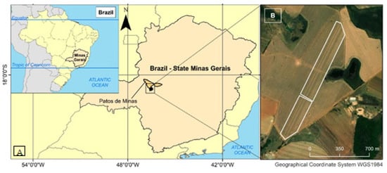
Figure 1.
(A) Location of the experiments in the municipality of Patos de Minas, MG e (B) Br1 top and Br2 bottom.
2.2. Experimental Outline
For Br1 and Br2, the experiments were performed using hybrid AG8088 PRO2, with spacing between plant lines of 0.5 m and plant distribution of three plants per meter. Thus, the spacing between plants was approximately 0.33 m, with an approximate density of 60,000 plants per hectare. Strips alternated between those without the application of A. brasilense (control group; STD) and those with the application of bioinoculant based on A. brasilense LBCC 0850 (treatment group, TS; 5 × 10⁻⁸ CFU/mL, 500 mL/ha) (Figure 2B,E). At the harvest stage, field yield data were measured using a CASE IH Axial Flow 6150 harvester.
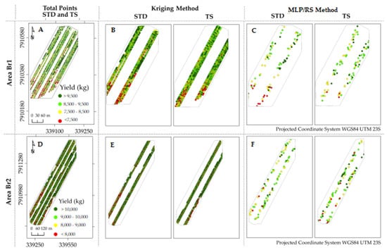
Figure 2.
Data of corn yield. (A,D)—Spatial distribution of corn yield samples after harvest differentiated by the application of A. brasilense (TS) or without treatment (STD), for areas Br1 and Br2, respectively. (B,E)—Yield data after filtering outliers for simulation of yield surfaces by Kriging for areas Br1 and Br2, respectively. (C,F)—Yield data for yield simulation by images for areas Br1 and Br2, respectively.
2.3. Acquisition of Yield Values
The yield data were directly obtained from the vector files of harvest provided by the machinery, by measuring the yield from measurements of mass and volume of the harvested product (Figure 2A,D). The harvester had load cells to measure the harvested load. Yield was estimated in tons per hectare at each meter of harvest.
The yield measurements were associated with a GNSS receiver, machine displacement, and cutting width systems. Additional sensors were also present in the sensor platform of the machines. These devices included humidity sensors, rotation sensors, and inclinometers that assisted the internal calibrations of the mechanisms of generation of georeferenced yield data.
The Differential Global Positioning System (DGPS) was used for positioning by GNSS. In this system, the relative positioning of the harvester occurs based on the correction of information obtained by a GPS receiver by the use of data from one or more fixed GPS receivers. In Brazil, a network of support towers receives the GPS signals and transmits the corrected signals through radio transmitters. For agricultural activities in which continuous positioning in real-time is required, the DGPS positioning provides coordinates with an accuracy of 1 to 3 m [17].
2.4. Filtering of Yield Data
Before generating surfaces and yield estimation models, the yield data were filtered for each area to eliminate outliers. A previously described method based on the Density-Based Spatial Clustering of Applications with Noise algorithm [18] was used for filtering. In addition, null yield data, plot border points, transition lines from one treatment to another, and locations where yield was within a confidence interval of +/− three standard deviations from the average yield of the area were excluded. The means, variation coefficients, minimum and maximum values, and grain yield asymmetries were determined to verify the normality of the measurements using Minitab version 19.2020 statistical software.
2.5. Generation of Yield Gain Surfaces by Kriging
The objective was to evaluate the application of a geostatistical technique (interpolation by Kriging) to perform yield inference considering different treatment scenarios in the study areas.
It is worth noting that the purpose of this analysis was to simulate the yield of the particular area, considering two situations: yield of an area that was not treated (STD) or treated with the application of A. brasilense (TS). For each area, two yield surfaces were generated considering different locations for interpolation. Initially, 80% of the points contained in the locations where treatment was not applied were considered for interpolation. Subsequently, 80% of the points contained in the locations where treatment was applied were considered (Figure 2B,E). The 20% of the remaining data distributed in each treatment were used to validate the models.
Before generating the interpolated surfaces, a semivariogram analysis was performed to define the mapping functions that best reproduced the yield structure analyzed. The spatial dependence between the data was modeled based on the semivariogram. This allowed the interpolation of productivity values at unsampled locations. Through the covariances, the statistical relationships existing between the spaced samples of successive predetermined values were measured, allowing the determination of the best linear combination of nearby sample values to estimate a value at an unknown location [7].
2.6. Generation of Yield Gain Surfaces from Spectral Models
Similar to the previous step, the spectral models were generated considering the yield of the area that was untreated or treated with A. brasilense.
2.6.1. Image Acquisition
High-resolution multispectral orbital images were obtained through remote orbital sensors from the PlanetScope satellite constellation two months before harvest during the floury grain production stage.
The choice of this phase is justified due to the greater correlation between the image bands and yield for this period compared to other phenological phases. The tests were performed in the preliminary stages of defining the final proposed method, such as described previously [19].
Regarding the sensor characteristics, PlanetScope satellite images have a spatial resolution of 3 m and radiometric resolution of 12 bits. The Bayer Mask CCD type PS2 sensor used in this constellation of satellites captures the wavelengths of blue (455–515 nm), green (500–590 nm), red (590–670 nm), and near-infrared (780–860 nm). The images are configured in the Universal Transverse Mercator projection system and World Geodetic System-84 horizontal datum and correction level 3B. The atmospherically corrected images are converted to surface reflectance.
2.6.2. Generation of Spectral Models for Yield Prediction
The values of band surface reflectance and multispectral index brightness were extracted through the generation of regions of interest using part of the points of the point-type vector files (Figure 2C,F). Each georeferenced yield value was related to the respective digital number in the image. It is important to note that the 100 sampling locations were randomly selected with a minimum distance of 5 m between adjacent locations. After selecting the points, we calculated the Pearson model between yield and spectral values from the images with the respective derived vegetation index.
We used the original bands of the PlanetScope imagery and the Normalized Difference Vegetation Index to generate the prediction models. We only used the original bands and index as predictor variables to avoid overfitting the generated models, which can occur when the number of parameters used in the regression is high.
Analogous to the Kriging step, yield surfaces were generated considering two scenarios: algorithms structured with yield and reflectance values derived only from areas that received treatment and from areas that did not receive treatment. Notably, the prediction models for Br1 and Br2 were not used to estimate yield outside the plot from which the training samples were extracted. Therefore, 80% and 20% of the samples were used for the training and validation of the algorithms, respectively.
In this step, the machine-learning algorithm used to generate the yield prediction models was the MLP Neural Network type. It was configured with three neurons in an intermediate layer. The learning rate was 0.3 and momentum was 0.2. This step was performed using Weka version 3.9.5 software (https://waikato.github.io/weka-wiki/downloading_weka/, accessed on 1 August 2021).
2.7. Model Validation
For validation and analysis of model accuracy, two metrics were used: MAPE% (Equation (1)):
where ŷ_i is the predicted value, y_i is the value observed in the field, and n is the total number of elements, and RMSE%) (Equation (2)):
where ŷ_i are the predicted values, y_i are the values measured in the field, and n is the total number of observations.
MAPE (%) = ((∑|ŷ_i − y_i|)/y_i)/n × 100
RMSE(%) = (√((∑(ŷ_i − y_i)2)/n) × 100)/((∑y_i)/n)
2.8. Generation of Yield Gain Surfaces
The yield gain surfaces were generated by subtraction between those simulated with the control and with the application of A. brasilense. To compare the surfaces generated, subtraction between the yield gain surfaces by Kriging and multispectral models was performed. The similarity between them was evaluated by Pearson’s correlation.
3. Results
Figure 3 presents the frequency diagram and descriptive statistics values from the yield data of the samples presented in Figure 2.
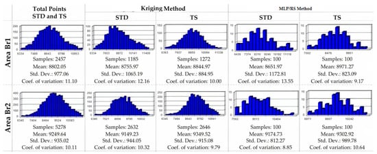
Figure 3.
Frequency diagram and descriptive statistics for study areas Br1 and Br2.
According to Figure 3, Br2 presented a higher yield and lower coefficient of variation (9249.64 Kg; 10.11%) than Br1 (8802.05 Kg; 11.10%). For both trials, from the samples used for Kriging and image models, a higher yield was observed in the sites where treatment was applied. From the samples used for Kriging, the productivities of the TS plots presented normality, with no normality in the STD data.
Figure 4 and Table 1 present data from the adjusted Kriging models and descriptive data of the semivariograms, such as the nugget effect, range, and path.
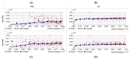
Figure 4.
Semivariograms for simulated surfaces: (A): Br1-STD; (B): Br1-TS; (C): Br2-STD; and (D): Br2-TS.

Table 1.
Descriptive data of semivariograms adjusted for BR1 and BR2 for STD and TS.
For the STD areas, the semivariograms fit to theoretical Gaussian and spherical models for the TS areas all obtained a lower error in the 110° direction. The semivariograms of the STD areas showed higher values than the TS areas for the nugget effect, range, and path, where the highest values were for STD Br1 (0.25, 4.68, and 0.80, respectively).
Figure 5 shows the performance graphs of the prediction models (RMSE%, MAPE%, and R2) by Kriging (Kriging Method) and by MLP from images obtained by remote sensing (RS). The yields obtained in the field and the abscissa axis are presented in the ordinate axis, the yield estimated by the models.
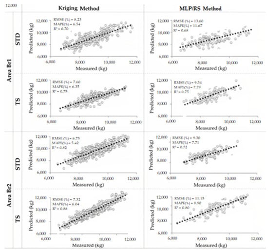
Figure 5.
Performance graphs of the prediction models for areas Br1 and Br2 by Kriging and MLP/RS methods from the sampled yield data.
When analyzing the Kriging performances, the models generated from samples from STD sites had a minimum RMSE% and MAPE% of 6.75 and 5.42, respectively, for Br2, compared to 7.32 and 6.04, respectively, for models generated from samples from TS sites. The prediction performances by MLP/RS indicated that the models generated from samples from STD sites had a minimum RMSE% and MAPE% of 9.30 and 7.71, respectively, for Br2. For the models generated from samples of the TS sites, the minimum RMSE% and MAPE% were 9.34 and 7.79, respectively, for Br1.
The correlation coefficients between estimated and measured yield for the models of estimation by Kriging varied from 0.70 to 0.88, respectively, whereas for the TS and STD sites in the Br2 area, maximum values were 0.88 and 0.82, respectively. For the models generated by neural networks, in Br2, the TS and STD treatments obtained the highest correlation coefficients (0.8 and 0.72, respectively).
Figure 6 shows the maps of corn yield gain by applying A. brasilense generated by the Kriging method and MLP/RS, and the comparison between the surfaces.
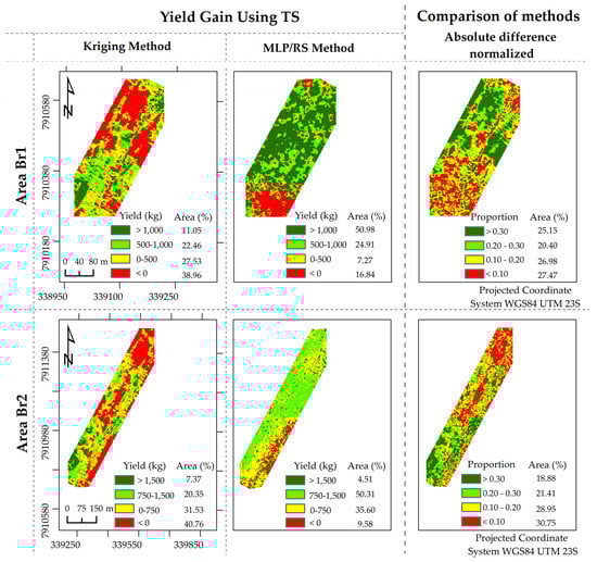
Figure 6.
Yield gain surfaces from Kriging and MLP/RS methods and comparison between surfaces for areas Br1 and Br2. Correlation between surfaces for Br1 = 53.04% and Br2 = 56.08%.
Analyses of the data of yield gain surfaces in Figure 6 indicated a more significant yield gain of surface generated by the MLP/RS method when A. brasilense was applied. In a general context, Kriging data revealed the distribution of areas that showed a gain mostly over the places where the treatments were applied. In contrast, the MLP technique indicated the yield gain throughout the entire area. The difference reflects the lower densification of points used for surface generation from the spectral model. There is an overestimation of the real value of yield gain due to the different amounts of samples used by different models in the generation of surfaces, culminating in similarities of 53.04% (Br1) and 56.08% (Br2) in the correlation between the methods.
4. Discussion
Regarding the behavior of regionalized variables (yield) when analyzing the samples separately (i.e., points derived from the TS and STD treatments), stationarity is evident. This is because in places under different management conditions, the expected yield values vary regularly in the surrounding area. In the analysis of the yield points considering the areas as a whole, the function presents characteristics of little stationarity (anisotropy). This condition is caused by the variability resulting from the different management techniques, in which A. brasilense is applied in alternate strips [20].
Spatial behaviors were evaluated by semivariograms adjusted to the Gaussian model in the cases of STD, and spherical for TS. The findings indicated the spatial dependence of all factors. Even with yield samples as a lower coefficient of variation, the Gaussian semivariogram infers that the yield of the STD area is an event with an apparent continuity greater than the yield defined by TS. In other words, the modeling of corn yield for these conditions cannot be modeled by parametric mathematical functions (linear regression). The difficulty of modeling STD plots is due to the variability and trend of yield conditioned to environmental factors, given that without treatment conditions, the crop is subject to biotic and abiotic factors [21].
For the plots treated with ST, the adjustment of spherical semivariograms with little dispersion in the plateau’s position reflects a normality condition in the probability distribution function (probability frequency diagrams, Figure 3) of the treated areas. This condition occurs given the application of A. brasilense, which was applied in the same amount along the TS plots, which reduced the variability caused by biotic and abiotic factors in the planting area [22].
Regarding biotic factors (exposure to pests, fungi, and insects) and abiotic factors (including climate, soil parameters, and topography), it is important to note that they were practically identical for both control and treatment locations. In this context, the only difference between the two sites was defined by management practices (an abiotic factor). This factor was decisive in the variability of yield and, consequently, in the modeling and performance of yield gain surfaces. We observed that applying A. brasilense to the crop resulted in lower variability in yield and reduced susceptibility to typical biotic factors affecting maize cultivation in tropical regions.
Regarding yield prediction, the models generated by Kriging were more accurate and less biased than those generated by images because they were modeled with a larger number of training samples. The precision and accuracy of Kriging are related to the distance and continuity between pairs of samples [23]. For the present study, the high density of yield data favored the generation of accurate and precise models.
The models generated by images had lower RMSE%, MAPE%, and R2 because they were trained on a considerably smaller contingent of yield samples. Furthermore, it should be considered that, unlike Kriging, the accuracy and precision of the models depend on the correlation between the bands and derived indices with yield and the spatial, spectral, and radiometric resolutions of the sensor [24].
The highest RMSE% and MAPE% errors observed in Br1 were associated with the fact that the area presented a higher coefficient of variation in yield (Figure 3). Another factor to consider is the spectral mixture, given the larger spacing between rows for this area, which is evidence of a greater response from the exposed soil. This condition occurs because the images used in the generation of the models were taken at the phenological stage of R1 in the corn crop, the phase in which the crop stabilized the vegetative development, and closing of the inter-row is defined.
The discrepancies between the yield gain maps generated by the different techniques are due to the nature of the modeling used in each technique. In the case of Kriging, yield is estimated as a function of spatial inference and as a function of distance and variance between pairs of samples. In contrast, for images, the yield distribution is inferred from the spectral response of pixels over the planting area.
5. Conclusions
With the increasing demand for the use of biostimulants in agricultural crops in search of increasingly sustainable and less environmentally harmful agriculture, based on techniques in geospatial data processing, we propose a methodology to show the gain in maize yield after applying biostimulants. Three conclusions can be made.
In conditions where it is not possible to evidence statistical differences between the yield of the control areas, based on the research methodology, it is possible to spatialize the yield gain following the application of A. brasilense. In conditions of mechanized harvesting with a high amount of georeferenced yield information, given the high accuracy and precision, we recommend using Kriging to generate the yield gain surfaces. Finally, under a few sample conditions, yield prediction models based on high spatial resolution images can be used to simulate yield gain surfaces with satisfactory precision and accuracy.
To achieve greater precision and accuracy, future studies should consider two aspects. The first is the possibility of generating the surfaces of yield gain from Kriging techniques. In this scenario, the models should consider agricultural variables not correlated to yield, that is, measures of agronomic parameters different from the variables currently available in the output file of the harvesters, where only agricultural variables highly correlated between themselves are presented. Secondly, for models generated by images, we highlight the need for sensors with higher spatial, spectral, and radiometric resolutions.
Author Contributions
Conceptualization, G.D.M., L.C.M.X., C.A.M.d.A.J. and G.P.d.O.; methodology, G.D.M., L.C.M.X., C.A.M.d.A.J. and G.P.d.O.; validation, B.S.V. and D.J.M.; formal analysis, G.D.M.; investigation, G.D.M., L.C.M.X., C.A.M.d.A.J., F.V.d.S. and G.P.d.O.; data curation, M.d.L.B.T.G.; writing—original draft preparation, G.D.M. and G.P.d.O.; writing—review and editing, M.d.L.B.T.G.; visualization, L.C.M.X.; supervision, G.D.M. and G.P.d.O.; project administration, G.D.M. and C.A.M.d.A.J. All authors have read and agreed to the published version of the manuscript.
Funding
This research received funding provided by Lallemand Plant Care.
Data Availability Statement
3rd Party Data and Restrictions apply to the availability of these data.
Conflicts of Interest
The authors declare no conflict of interest.
References
- Scott, S.; Housh, A.; Powell, G.; Anstaett, A.; Gerheart, A.; Benoit, M.; Wilder, S.; Schueller, M.; Ferrieri, R. Crop yield, ferritin, and Fe(II) boosted by Azospirillum brasilense (HM053) in corn. Agronomy 2020, 10, 394. [Google Scholar] [CrossRef]
- Caradonia, F.; Buti, M.; Flore, A.; Gatti, R.; Morcia, C.; Terzi, V.; Ronga, D.; Moulin, L.; Francia, E.; Milc, J.A. Characterization of leaf transcriptome of grafted tomato seedlings after rhizospheric inoculation with Azospirillum baldaniorum or Paraburkholderia graminis. Agronomy 2022, 12, 2537. [Google Scholar] [CrossRef]
- Mattos, M.L.T.; Valgas, R.A.; Martins, J.F.S. Evaluation of the agronomic efficiency of Azospirillum brasilense strains Ab-V5 and Ab-V6 in flood-irrigated rice. Agronomy 2022, 12, 3047. [Google Scholar] [CrossRef]
- Picazevicz, A.A.; Kusdra, J.F.; Moreno, A.d.L. Maize growth in response to Azospirillum brasilense, Rhizobium tropici, molybdenum and nitrogen. Rev. Bras. De Eng. Agrícola E Ambient. 2017, 9, 623–626. [Google Scholar] [CrossRef]
- Thai, T.H.; Omari, R.A.; Barkusky, D.; Bellingrath-Mimura, S.D. Statistical Analysis versus the M5P Machine Learning Algorithm to Analyze the Yield of Winter Wheat in a Long-Term Fertilizer Experiment. Agronomy 2020, 10, 1779. [Google Scholar] [CrossRef]
- Panagopoulos, T.; Jesus, J.; Ben-asher, J. Tools for optimizing management of a spatially variable organic field. Agronomy 2015, 5, 89–106. [Google Scholar] [CrossRef]
- Ma, Y.; Zhang, Z.; Kang, Y.; Özdoğan, M. Corn yield prediction and uncertainty analysis based on remotely sensed variables using a Bayesian neural network approach. Remote Sens. Environ. 2021, 259, 112408. [Google Scholar] [CrossRef]
- Ridwan, M.A.; Radzi, N.A.M.; Ahmad, W.S.H.M.W.; Mustafa, I.S.; Din, N.M.; Jalil, Y.E.; Zaki, W.M.D.W. Applications of Landsat-8 data: A Survey. Internat. J. Eng. Technol. 2018, 7, 436–441. Available online: http://dspace.uniten.edu.my/jspui/handle/123456789/11607 (accessed on 20 January 2023). [CrossRef]
- Hall, O.; Wahab, I. The use of drones in the spatial social sciences. Drones 2021, 5, 112. [Google Scholar] [CrossRef]
- García-Martínez, H.; Flores-Magdaleno, H.; Ascencio-Hernández, R.; Khalil-Gardezi, A.; Tijerina-Chávez, L.; Mancilla-Villa, O.R.; Vázquez-Peña, M.A. Corn grain yield estimation from vegetation indices, canopy cover, plant density, and a neural network using multispectral and RGB images acquired with unmanned aerial vehicles. Agriculture 2020, 10, 277. [Google Scholar] [CrossRef]
- Wang, L.; Wang, P.; Liang, S.; Zhu, Y.; Khan, J.; Fang, S. Monitoring maize growth on the North China Plain using a hybrid genetic algorithm-based back-propagation neural network model. Comput. Electr. Agric. 2020, 170, 105238. [Google Scholar] [CrossRef]
- Maresma, A.; Chamberlain, L.; Tagarakis, A.; Kharel, T.; Godwin, G.; Czymmek, K.J.; Ketterings, Q.M. Accuracy of NDVI-derived corn yield predictions is impacted by time of sensing. Comput. Electr. Agric. 2020, 169, 105236. [Google Scholar] [CrossRef]
- Khanal, S.; Fulton, J.; Klopfenstein, A.; Douridas, N.; Shearer, S. Integration of high resolution remotely sensed data and machine learning techniques for spatial prediction of soil properties and corn yield. Comput. Electr. Agric. 2018, 153, 213–225. [Google Scholar] [CrossRef]
- Brown, M.R.; Blackburn, S.I. Biofuels from microalgae. Sustain. Energy Solut. Agric. 2014, 277, 277–321. [Google Scholar]
- Baum, M.E.; Archontoulis, S.V.; Licht, M.A. Planting date, hybrid maturity, and weather effects on maize yield and crop stage. Agron. J. 2019, 111, 303–313. [Google Scholar] [CrossRef]
- Pereira Filho, I.A.; Borghi, E. Mercado de Sementes de Milho no Brasil: Safra 2016/2017. Embrapa 2016, 28. Available online: http://www.infoteca.cnptia.embrapa.br/infoteca/handle/doc/1060346 (accessed on 20 January 2023).
- Vadakke Veettil, S.; Aquino, M.; Marques, H.A.; Moraes, A. Mitigation of ionospheric scintillation effects on GNSS precise point positioning (PPP) at low latitudes. J. Geod. 2020, 94, 15. [Google Scholar] [CrossRef]
- Leroux, C.; Jones, H.; Clenet, A.; Dreux, B.; Becu, M.; Tisseyre, B. A general method to filter out defective spatial observations from yield mapping datasets. Precis. Agric. 2018, 19, 789–808. [Google Scholar] [CrossRef]
- Webster, R.; Oliver, M.A. Geostatistics for Environmental Scientists; John Wiley & Sons: Hoboken, NJ, USA, 2007. [Google Scholar]
- Radočaj, D.; Jug, I.; Vukadinović, V.; Juriłić, M.; Gałparović, M. The effect of soil sampling density and spatial autocorrelation on interpolation accuracy of chemical soil properties in arable cropland. Agronomy 2021, 11, 2430. [Google Scholar] [CrossRef]
- Madugundu, R.; Al-Gaadi, K.A.; Tola, E.; Zeyada, A.M.; Alameen, A.A.; Edrris, M.K.; Mahjoop, O. Impact of Field Topography and Soil Characteristics on the Productivity of Alfalfa and Rhodes Grass: RTK-GPS Survey and GIS Approach. Agronomy 2022, 12, 2918. [Google Scholar] [CrossRef]
- Zou, R.; Zhang, Y.; Hu, Y.; Wang, L.; Xie, Y.; Liu, L.; Yang, H.; Liao, J. Spatial variation and influencing factors of trace elements in farmland in a lateritic red soil region of China. Agronomy 2022, 12, 478. [Google Scholar] [CrossRef]
- Pereira, F.V.; Martins, G.D.; Vieira, B.S.; de Assis, G.A.; Orlando, V.S.W. Multispectral images for monitoring the physiological parameters of coffee plants under different treatments against nematodes. Precis. Agric. 2022, 23, 2312–2344. [Google Scholar] [CrossRef]
- Pereira, G.W.; Valente, D.S.M.; Queiroz, D.M.D.; Coelho, A.L.D.F.; Costa, M.M.; Grift, T. Smart-map: An open-source QGIS plugin for digital mapping using machine learning techniques and ordinary kriging. Agronomy 2022, 12, 1350. [Google Scholar] [CrossRef]


Disclaimer/Publisher’s Note: The statements, opinions and data contained in all publications are solely those of the individual author(s) and contributor(s) and not of MDPI and/or the editor(s). MDPI and/or the editor(s) disclaim responsibility for any injury to people or property resulting from any ideas, methods, instructions or products referred to in the content. |
© 2023 by the authors. Licensee MDPI, Basel, Switzerland. This article is an open access article distributed under the terms and conditions of the Creative Commons Attribution (CC BY) license (https://creativecommons.org/licenses/by/4.0/).