Abstract
Deep learning excels in the identification of specific plant diseases. However, dealing with multi-domain datasets, which encompass a variety of categories, presents challenges due to limited data availability. (1) Background: In real-world scenarios, data distribution is uneven, the scale continues to grow, new categories emerge, and a phenomenon known as ‘catastrophic forgetting’ occurs. Models rely on a substantial amount of data for labeling and training. (2) Methods: We introduce a two-stage approach. The first stage is the scalable feature learning phase, where the previous feature representation is fixed. Through a new feature extractor, incoming and stored data are trained to expand features. In the second stage, by introducing an auxiliary loss to determine whether key parameters are retained, we reduce the instability of weight parameters. This maintains the separability of old features and encourages the model to learn new concepts, diversity, and discriminative features. (3) Results: Our findings indicate that when the data landscape shifts, recognition accuracy in multi-task continual learning, leveraging the simultaneous availability of datasets, significantly outperforms single convolutional networks and multi-task learning models. (4) Conclusions: Our method advances continual learning towards practical applications. It is particularly effective in mitigating catastrophic forgetting in multi-domain datasets and enhancing the robustness of deep-learning models.
1. Introduction
In agricultural and forestry cultivation, diseases constitute a key factor influencing the quality of plant growth [1]. Diseases not only directly lead to crop yield losses and restrict plant growth but also pose food safety concerns [2,3]. In recent years, due to factors such as climate change, influences of cultivation practices, and variations in ecological environments and plant varieties, plant diseases and pests have become more prevalent, significantly impacting crop yield and quality [4,5,6]. Accurate identification of plant leaf disease categories is a fundamental prerequisite for enhancing the efficiency of plant disease control efforts [7]. Therefore, the early detection of plant diseases and timely mitigation are indispensable measures for the agricultural and forestry sectors.
In the traditional process of diagnosing plant diseases, leaf diseases are often identified by experts, requiring a significant amount of manpower and time. This method is inefficient and costly. Additionally, plant growth is seasonal, and traditional identification methods cannot accurately and comprehensively reflect the types and manifestations of diseases [8]. Therefore, we should focus our research on aspects such as rapid detection, precise identification, and cost reduction in the study of plant diseases [9].
Precision agriculture utilizes cutting-edge technologies to optimize decision-making processes [10,11]. Thanks to contemporary digital technologies, a vast amount of data is collected in real-time, and various machine-learning (ML) algorithms are employed to provide optimal decisions, thereby minimizing costs. However, there is still room for improvement in this field, especially in decision support systems that contribute to transforming large amounts of data into useful recommendations. Algorithms and methods such as linear regression, logistic regression, random forests, Gaussian models, decision trees (DT), naive Bayes (NB), k-nearest neighbors (KNN), and support vector machines (SVM) are commonly employed in this context.
As deep learning research continues to advance, convolutional neural networks (CNN), used for image classification, have become a core focus in the field of computer vision [12]. The application of deep learning in the agricultural sector is also becoming increasingly widespread. With the development of artificial intelligence and computer vision, new solutions are being brought to plant disease detection [13,14]. These methods can provide more accurate predictions than traditional approaches, leading to better decision making.
Ji et al. mentioned a joint convolutional neural network for the identification of grape plant diseases with a focus on feature extraction [15]. Advanced feature fusion enhanced the representational potential of the joint model, enabling it to outperform its competitors in grape leaf disease identification. To detect plant diseases such as black rot, mycorrhiza, and rust, Guo et al. proposed a deep-learning-based model that improves accuracy, generalizability, and training effectiveness. The model places emphasis on the utilization of a region proposal network (RPN) on a dataset of diseased leaves to identify and locate unhealthy leaves. Subsequently, features are extracted using the Chan–Vese (CV) algorithm. The final accuracy of disease detection using the transfer learning model was 83.57% [16]. Gadekalu et al. introduced a hybrid PCA technique for feature extraction and assessed the data for superiority and accuracy using the whale optimization algorithm [17].
Nagaraju and Chawla utilized deep-learning models for the automatic identification of diseases through hyperspectral images, addressing the limitations in classification. They also identified challenging issues, such as the insufficiency of adapting new computer vision techniques for automatic disease detection, the impact of environmental conditions on disease classification analysis during data acquisition, the lack of well-defined disease symptoms, and the difficulty in setting visual similarities between healthy and diseased components and symptoms. These challenges often lead existing methods to rely on variation for differentiation [18]. Jasim and Tuwaijari presented a system for classifying and detecting plant leaf diseases using convolutional neural networks, achieving training and testing accuracies of 98.29% and 98.03% for all datasets, respectively. Their work focused on specific plant types, namely tomatoes, peppers, and potatoes, from the Plant Village dataset, which contains 20,636 plant images and classifies 15 plant leaf diseases [19]. Arsenovic et al. discussed the limitations and drawbacks of existing plant disease detection models. They introduced a new dataset containing 79,265 images of tree leaves in natural environments. The researchers proposed a new two-stage neural network-based architecture for plant disease classification, achieving an accuracy of 93.67% [20]. Atila et al. explored an automated model for detecting and classifying unhealthy areas of plants. To detect various diseases in plant leaves, they compared the accuracy of an efficient CNN-based network state-of-the-art model with other structures. The model achieved an accuracy of 96.18% in comparison to different architectures [21].
However, with the increasing computational power today, deep-learning models have become more powerful, yielding stronger results, and various deep networks have emerged. Nevertheless, they lack universality in identifying plant diseases [22]. The deeper the network, the more information about crucial features of the model is lost, which is undesirable when precise features are needed for classification [23]. In many cases, data collection is performed in laboratory environments, providing simplistic background data. Disease features often concentrate in the central region of the images. Therefore, models trained on such images struggle to handle those captured in natural, real-world conditions (e.g., outdoor settings). Obstacles in image recognition arise due to different angles, lighting conditions, collection times, distances, and variations in leaf conditions. Moreover, these models face limitations such as high computational complexity, execution time, and costs, as well as limited adaptability in diverse plant disease datasets spanning multiple fields. This renders a singular convolutional neural network model highly vulnerable, leading to a significant performance decrease when confronted with the influx of new sample categories [24]. Therefore, there is an urgent need to develop a more effective and efficient universal model for sustainable early detection of plant diseases, aiming to reduce implementation time and costs.
Addressing the limitations of traditional agriculture and deep learning in the field of plant pathology, in this paper, we propose a two-stage multi-task continual learning approach for plant disease detection. In the first stage of multi-task continual learning, we train the deep-learning model using cross-entropy loss. In the second stage, we train the deep-learning model with auxiliary loss. By comparing the effects of various network models in both deep learning and continual learning, we demonstrate a significant improvement in the accuracy and detection speed of plant disease detection achieved by our proposed model.
The contributions of this paper mainly lie in the following aspects:
- (1)
- Used leaves captured and collected from the real environment as the experimental dataset;
- (2)
- Proposed a novel two-stage continual learning method that reduces redundant parameters within the model to train on new classes, allowing the model to learn new tasks on top of the existing ones;
- (3)
- Compared to traditional deep learning, the new two-stage continual learning method can detect plant diseases more rapidly and accurately.
The rest of this paper is organized as follows: Section 2 delves into the principles of the dataset and continual learning. In Section 3, we provide a detailed exposition of the experimental results, followed by discussion and analysis. Section 4 analyzes the challenges of knowledge transfer and outlines the current limitations and future work. Finally, Section 5 emphasizes the strengths of this research.
2. Dataset and Methods
2.1. Dataset
This paper utilized leaf images captured and collected from real environments as experimental data. The dataset includes healthy leaves from three different species and unhealthy leaves affected by various diseases. A total of 10 categories of sample data and 1605 images were selected for training after data pre-processing. Some images were sourced from the Kaggle competition (https://www.kaggle.com/competitions/plant-pathology-2020-fgvc7), accessed on 6 May 2022. It is worth noting that some of these images contained background information, which may have had an impact on the model’s performance in the experiments. Table 1 displays the species and the number of healthy leaves, with the minimum number of images for these species being 117 and the maximum number being 188. Table 2 provides information on the number of diseases and images for each diseased leaf, revealing an imbalance in the number of available leaf images. The samples are illustrated in Figure 1. We employed the Holdout cross-validation technique for data splitting. We divided the original dataset into a training set and a validation set with a 7:3 ratio. The training set was used to train the model, while the validation set was used to assess the model’s performance.

Table 1.
Experimental dataset.
Table 2.
Name and number of samples in the dataset.
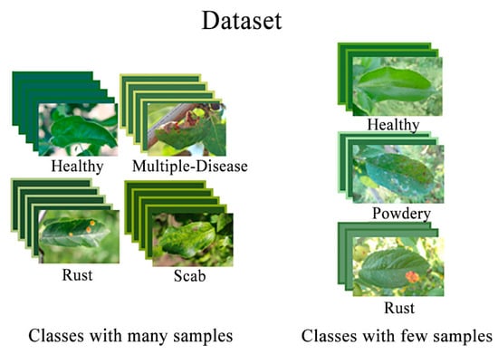
Figure 1.
Sample graph of the dataset.
2.2. Methods
2.2.1. Catastrophic Forgetting
In the context of deep learning, model parameters are typically updated using gradient descent methods. These model parameters are continuously iteratively updated during forward and backward propagation. However, the training process must be restarted whenever new data become available. This approach quickly becomes challenging in handling the data stream and cannot be applied in the long term due to storage limitations or privacy issues. In machine learning, when learning new tasks, the network’s weights are adjusted to accommodate new data. However, this adjustment may disrupt the knowledge represented by the existing weights for old tasks. In simple terms, due to shared parameters, the new learning process can “overwrite” the old knowledge. This is known as catastrophic forgetting [25]. On one hand, a learning system should be capable of acquiring new knowledge and refining existing knowledge based on continuous input to overcome catastrophic forgetting. On the other hand, it should prevent significant interference of new input with existing knowledge. Therefore, the continual learning of multiple tasks remains the primary challenge in deep learning.
There are three main approaches to overcoming the problem of catastrophic forgetting: replay-based approaches, regularization-based approaches, and parameter isolation approaches [26]. Among the regularization-based methods, Li et al. [27] utilize knowledge distillation, Dhar et al. [28] enhance knowledge distillation by increasing attention loss, while Kirkpatrick et al. [29] and Zenke et al. [30] estimate the importance of network parameters and penalize changes in essential parameters. Parameter isolation methods are computationally expensive and require access to task identifiers. Both replay and regularization-based methods can be used for continual learning models. However, the former has memory requirements comparable to the size of current deep networks in addition to network parameters, and it has not been effectively addressed for class-incremental classification problems [31].
From the Figure 2, we can observe that the model exhibits a certain degree of forgetfulness about prior knowledge. This is evident in the classification accuracy, with the first six samples showing a much lower accuracy compared to the last four samples.
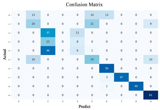
Figure 2.
Catastrophic forgetting in deep learning. The darker the color along the diagonal of the confusion matrix, the more accurate the predictions, indicating stronger generalization performance of the trained model.
2.2.2. Principles of Continual Learning
Continual learning aims to extract knowledge from a stream of information and then build a knowledge memory to improve future predictions. The concept involves creating a system that summarizes various prediction tasks and potential data patterns, preserving task-specific knowledge for each task that can be retrieved and applied when encountering similar tasks later [32]. This is evident in the model’s ability to retain its performance on the original task when exposed to new data. Furthermore, the model can effectively handle recent data categories without any restrictions on the order of category arrivals, as illustrated in Figure 3.
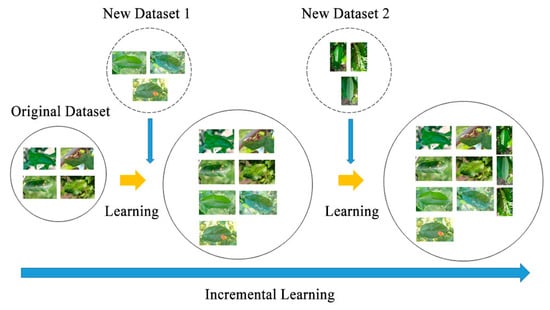
Figure 3.
The process of the multi-task continual learning system.
In a continual learning process, the network model observes a set of categories and the training data corresponding to them . In particular, the dataset at step t has data in the format , where is the input image, and is within the set of labels . The label space of the model encompasses all visible categories, denoted as , and the model is expected to predict all the categories in these datasets effectively.
When the model is trained to a particular stage, and the value of the loss function no longer decreases significantly, the model parameters can be considered to have converged to a local optimum point. At this point, the model performs better on the current task [33]. In an already-trained model, some parameters are essential for the current task, while others are not. If these critical parameters are changed randomly, the model’s performance on the corresponding task may fluctuate drastically. Therefore, when using a trained model for a new task, to ensure that the model does not perform poorly on the previous task, it is necessary to limit the extent of changes in those parameters that are more important for the historical task. This means that the parameters crucial for the historical task should not undergo significant changes during the learning process of the new task. The aforementioned idea can be translated into an equation and expressed as
where represents the overall loss function during the current task’s learning process, is the initial loss function for the current task, λ is the weighting factor used to assess the importance of both the current and historical tasks, is the level of significance of the ith parameter within the descriptive model of the historical task, is the ith parameter within the model, and is the ith parameter within the final model obtained upon completing the previous task.
In the case of more than one historical task, a common term of loss needs to be added to the overall loss function for each historical task while the current task is being learned. For example, when the number of historical tasks is two, the overall loss function takes the form of
where is the weighting factor used to measure the importance of Historical Task 1, and is the weight coefficient used to measure the importance of Historical Task 2, and is the degree of importance of the ith parameter of the characterization model for Historical Task 1, and is the importance of the ith parameter of the model for Historical Task 2, and is the ith parameter of the final model obtained at the end of the learning of Historical Task 1, and is the ith parameter in the final model obtained at the end of learning Historical Task 2. For the contribution of and to the loss function, (i) if the source and target are more similar, a larger was chosen to constrain the weight changes, since small changes may be sufficient to fit; (ii) if more target data are given, a smaller is chosen, and a larger is used.
In a system of methods based on parameter regularization, the focus is on how to determine the coefficients , i.e., how to determine the importance of a parameter in the model for the task at hand. The Fisher information matrix entries for each parameter are obtained by summing all the gradients for that parameter and then dividing by the total number of samples.
2.2.3. Neural Network Architecture for Continual Learning
The decomposition of the parameter updates serves as the foundation for our investigation of the quadratic regularization function mechanism. Specifically, to calculate the gradient of Equation (2), we perform the parameter update as follows for
where is the loss of the task , is the regularization constant, is the parameter at the end of the previous task, and η denotes the learning rate of the overall model. We assume the importance score matches the empirical configuration of the typical quadratic regularization function. This is used to adjust the current task during training. is the gradient for the specific task loss . ⊙ represents the interpolation operation. To guarantee that the random interpolation of the current and prior values of the parameters achieves a minimal loss on recent and previous tasks, the model parameters can be regularized when learning a new task. This strategy dramatically mitigates catastrophic forgetting. We rearrange Equation (3) as follows.
The above equations suggest that parameter updating under quadratic regularization can be decomposed into two simultaneous operations: (1) using interpolation between the current values of the model parameters and the values at the end of the previous task to constrain changes in the model parameters in any given iteration (sum of the first two items); and (2) using model parameter movement along a task-specific gradient to learn new tasks (item after the minus sign). Interpolation changes the learning rate over multiple iterations The quadratic regularization function changes the learning rate of the parameters. If the importance of the parameter is high, the value of becomes smaller, thus reducing the effective learning rate of the parameter and limiting its variability. If the importance of the parameter is low, the value of remains essentially the same. The interpolation process alters the learning rate in multiple iterations, allowing it to alter according to the gradient and to learn new tasks.
Figure 4 represents the model diagram for the extensible feature learning stage, which is the first phase of continual learning optimization. The extensible feature extractor is established by combining the newly created feature extractor with the extended feature extractor . Specifically, for a given image x∈, the features u extracted in step t are combined using Equation (5).
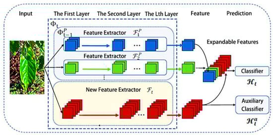
Figure 4.
Scalable feature learning phase.
In this context, the notation signifies the combination of both old and new feature extractors. The model employs the previous feature extractors ,…, to learn from existing knowledge while encouraging the new feature extractor to focus on learning novel aspects of new classes. Subsequently, the features are fed into the classifier for prediction, as shown in Equation (6):
Thus, the predicted value is the index of the maximum value for , and represents the prediction for the class . The classifier is designed to match the input and output dimensions for step . The parameters of associated with old features are inherited from to retain previous knowledge, while its newly added parameters are initialized randomly.
To mitigate catastrophic forgetting, the model freezes the learned function at step , as it captures the inherent structure of previous data. Specifically, the parameters of the final super feature extractor and the batch normalization statistics are not updated. Additionally, this work utilizes as an initialization instance to reutilize prior knowledge for achieving rapid adaptation and forward propagation.
When used for classification and recognition in the context of new feature domain learning, classifiers exhibit bias. Our improvement method takes into account the distribution differences between the source domain and the new feature domain, based on the source domain classification error. We achieve this by incorporating features extracted by the new feature extractor as an auxiliary loss into the network’s overall loss, reducing the drift of source domain data and new feature domain data within the network. This, in turn, optimizes the distribution error for the new feature domain data. The weights for expandable features need to be re-estimated at each iteration to ensure that the weights are continually updated, enabling the network to adapt to data variations. We trained a cross-entropy loss model on memory and input data as follows:
where represents the input image, and is the corresponding label. means the probability of correct prediction. represents the image region. The region size is applied to normalize this formula.
To eliminate model redundancy and maintain a compact representation based on the complexity of new sample features, we used a channel-level masking method. This method involves dynamically expanding the super feature extractor to prune filters in the feature extractor , where these masks are jointly learned with the feature representation. Each feature map constructs a mask, where the mask values are close to one for pixels resembling the lesion and close to zero for pixels resembling the background or noise. Assuming the model can accommodate up to n tasks, a Bernoulli binomial distribution is used in each training batch to generate masks, selecting 1/n of the parameters for the task being trained, while the remaining parameters are frozen. The goal of this work is to maximize the utilization of parameters in the model for optimal performance. After training on the current batch is completed, the model parameters are reset, and a new mask is generated to select another 1/n of the parameters for training. The mask learning process divides a convolutional layer into two regions based on a predefined dropout rate, where one part is trainable, and the other part is fixed. Filters are added after the trainable part to filter out the gradients that would update the fixed parameters during backpropagation.
At the beginning of the training cycle, all channels are activated uniformly. As the batch index increases, the masks gradually become binary during a training epoch. Training deep-learning models for image detection involves a significant computational workload when processing images. To eliminate model redundancy and maintain a compact feature representation, the feature learning stage in this paper controls the information flow by constructing masks for the feature maps, enhancing relevant information while suppressing irrelevant negative information. Furthermore, the model learning process is incremental, allowing this module to be iteratively optimized multiple times. For the new feature extractor , the input feature maps for a given image in convolutional layer are represented as , introducing the channel masks to control the size of the layer l, where ∈[0, 1], and is the number of channels in the layer . Mask modulation is described in Equation (8):
where represents the feature map with masks, and ⊙ denotes channel-wise multiplication. To ensure that the values of fall within the interval [0, 1], a gating function is employed, as described in Equation (9):
where represents the learnable mask parameters, and the gating function in this work employs the Sigmoid function. With this masking mechanism in place, the super feature for step can be rewritten as shown in Equation (10):
The author uses channel-level mask pruning to trim dynamic fusion feature representations, reducing network parameters and alleviating the vanishing gradient problem, achieving improved accuracy in plant disease classification.
In the second stage, the proposed framework is trained to recognize plant diseases across different datasets. To identify various classes of diseases on different types of leaves, the proposed framework penalizes the classification model in each training increment using the function. These leaves come from separate datasets because our datasets were collected using various methods, resulting in different leaf shapes and various disease patterns. The second-stage classifier recognizes a label space of to encourage the network to learn the function of distinguishing between old and new concepts. This label space includes a set of new categories and other categories, treating all old concepts as a single category. Therefore, the introduction of an auxiliary loss results in the following expandable feature loss.
where is the hyperparameter that controls the auxiliary loss function. It is worth noting that for the original dataset of the first stage t = 1, = 0.
From Figure 5, we can clearly observe that in the standard training model, deep-learning model, and continual learning model, the introduction of auxiliary loss leads to a significant improvement in accuracy compared to when auxiliary loss is not introduced.
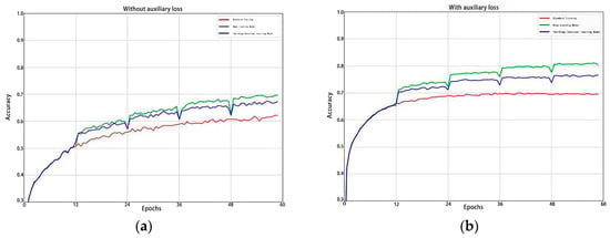
Figure 5.
(a) Without introducing auxiliary loss; (b) introducing auxiliary loss.
The proposed model framework is trained to recognize plant diseases in various datasets during the second training stage. Although the training technique is the same, the proposed framework’s classification model is penalized in each incremental training (by ) in order to identify different disease classes from the dataset. The new input images come from a different dataset and show different types of abnormal disease patterns. The model is improved by minimizing the objective function in the , learning such diverse classification tasks without catastrophically forgetting its prior knowledge. The loss function optimizes the classification model, which outperforms some incremental learning schemes.
3. Results
In this section, we conduct a large number of experiments to validate the effectiveness of our algorithm. We evaluate our method on three datasets using two training mechanisms. In the following, we will first present the experimental setup and implementation details in Section 3.1, followed by offering the experimental results of the algorithm on the datasets in Section 3.2. We also present the evaluation results of the confusion matrix and provide a detailed explanation.
3.1. Experimental Setup and Implementation Details
In the experiments, a multi-tasking plant disease identification and classification study was carried out using PyCharm software. The Python language was chosen, and the Pytorch framework in PyCharm software was utilized. The experiments were con-ducted using ubuntu 16.04, a server with 11 GB of RAM, an Intel-i7 processor, and an NVIDIA GeForce GTX 1080 Ti graphics card.
Continual learning employs a two-stage training methodology, with the goal of enhancing the model’s adaptability to acquire new information from different tasks at various times, while retaining details from previous tasks. We employed three deep-learning models for comparison: VGG, ResNet, and DenseNet. The features extracted using the CNN network are 224 × 224 pixels The SGD optimizer was used in both training phases, with the momentum set to 0.5 and the weight decay term set to 0.0005.
To ensure a fair comparison of experimental results and validate the feasibility of the proposed two-stage continual learning method, the parameters of the deep-learning models were standardized, and experimental hyperparameters were normalized. In the first stage, the recognition model is trained using the original dataset, with cross-entropy loss selected as the loss function and the batch size set to 32. The network is trained for 60 epochs with an initial learning rate of 0.01. Starting from the 30th epoch, the learning rate decreases to 1/10 of the previous period every 10 epochs. This learning rate reduction continues for 30 epochs. The training hyperparameters are the same as the baseline. In the second stage, the batch size for dataset training was adjusted to 16, and the learning rate was set to 0.001, with the number of training epochs remaining at 60.
Two approaches to machine learning were used for training: firstly, training the training set from scratch involves deep learning. Secondly, training the network model continuously, the difference between the two approaches is whether there are constraints on the parameters. This paper analyzes the performance of the two training mechanisms on a training-test dataset.
To ensure the fairness and reliability of the test results, after several rounds of debugging, the uniform hyperparameters are shown in Table 3.
Table 3.
Hyperparameter settings.
3.2. Assessment on F1 Scores and Loss Values
The F1 score and loss values were chosen to evaluate our model. The F1 score is a classification metric, defined as the summed average of precision and recall, which combines the outputs of precision and recall. Our F1 score is computed for both phases in this evaluation section. The F1 score is calculated after computing precision and recall for each class in the current stage, as shown in Equation (9), and then averaged to represent the learning performance of both phases. In the next section, we will use the confusion matrix to assess the overall learning performance of the model. Changes in the loss value indicate if the model can be trained further. The training loss continues to decrease, and the validation loss also decreases, indicating that the network is still learning.
The first stage used four different sample types in the original dataset, while the second stage employed six different sample types in the new dataset. The F1 scores for the two stages were 92.87 and 94.65, with corresponding loss values of 0.153 and 0.106, as depicted in Figure 6. While both stages exhibit an enhancement in learning capacity, the second stage displays fluctuations in the model’s learning curve, possibly influenced by the parameters carried over from the first stage. The parameters that are modified during the learning of new samples will be updated based on the most recent sample data, especially those crucial for model recognition. This updating process can significantly impact the characteristics of previously acquired information. Table 4 shows the recognition accuracies of standard deep learning and continual learning in addition to the three network models VGG11, ResNet18, and DenseNet121. Where “-" means that in the general deep learning models, the dataset was not trained separately according to plant categories.
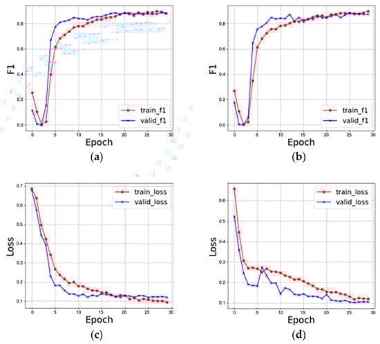
Figure 6.
F1 score and loss value in two stages: (a) F1 score in the first stage; (b) F1 score in the second stage; (c) loss value in the first stage; (d) loss value in the second stage.
Table 4.
Recognition accuracies of ordinary deep learning and continual learning (%).
The authors analyze our method for continual learning using confusion matrices. In general, the darker the color along the diagonal of the confusion matrix, the more accurate the predictions, indicating the stronger generalization performance of the trained model. The ten disease categories are represented by the horizontal and vertical coordinates in the confusion matrix, where the horizontal coordinate corresponds to the true label, and the vertical coordinate corresponds to the anticipated label. The evaluation samples are represented as e1 through e10 in the following order: Healthy (Apple), Multiple-Disease (Apple), Rust (Apple), Scab (Apple), Healthy (Pear), Rust (Pear), Powdery (Pear), Healthy (Coffee), Rust (Coffee), and Red Spider Mite (Coffee). There is no corresponding learning accuracy for the individual datasets on the three networks, as general deep learning does not involve staged learning. Therefore, we only provide the overall average accuracy. In contrast, we demonstrate its capacity for continual learning in Figure 7 using confusion matrices for each network.
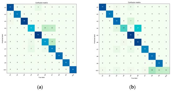
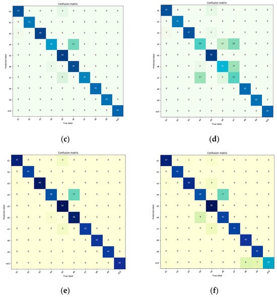
Figure 7.
For the confusion matrix, the darker the color on the diagonal, the more accurate the predictions, indicating stronger generalization performance of the trained model. (a) VGG11 with CL (continual learning); (b) VGG11 with DL (general deep learning); (c) ResNet18 with CL; (d) ResNet18 with DL; (e) DenseNet121 with CL; (f) DenseNet121 with DL.
From Figure 7, it can be observed that when the VGG11 network was directly applied to plant disease detection classification, it achieved an accuracy of only 82.35%. However, when the VGG11 network was enhanced with the continual learning mechanism, it improved its recognition accuracy by 9.06%, resulting in an accuracy of 89.81%. The ResNet18 network, after incorporating the continual learning mechanism, yielded significant results, with classification accuracy increasing from 83.22% to 93.84%, a 12.76% improvement. Similarly, the DenseNet121 network, when integrated with the continual learning mechanism, saw its classification accuracy rise from 88.53% to 94.47%, marking a 6.71% improvement.
4. Discussion
4.1. Challenges in Knowledge Transfer
We found from the results that the trained model will have about a 10% improvement in overall recognition accuracy compared to the traditional deep-learning model. Still, during the transition from the original dataset to the new dataset, the model will decrease in recognition accuracy. It may be because the weight changes fluctuate significantly in the early stages of knowledge transfer. It is somewhat challenging to find a balanced relationship between memory and updating. When the model starts a new feature recognition, the feature distribution of the current actual image is closer to the feature distribution of the previous real image (even if they do not belong to the same class). In other words, inter-class similarity leads to a possible bias at the prediction time. For example, apple trees may be affected by various fungal and bacterial diseases, leading to the appearance of similar spots on the leaves, such as black spot disease, powdery mildew, or rust. These spots may exhibit visual similarities, increasing inter-class similarity. However, as the learning progresses, we introduce auxiliary losses to overcome this error, using the redundancy of parameters, first using the criteria we set to keep the more essential parts of the parameters for the original dataset, such that the classifier will produce a reasonable response to these parameters. When the model starts learning new data again, we selectively update those parameters that are not important for the historical data, seeking the balance of stability and plasticity.
4.2. Current Limitations and Future Work
However, there are still some limitations in the current research. Firstly, the experiments are primarily conducted in artificial forests, taking into account some real-world factors, but further in-depth consideration and research are needed for a broader range of environmental factors. Therefore, the next steps in research could involve validating algorithm accuracy and optimizing the algorithm in complex natural forest environments. Secondly, it could be considered to combine feature visualization and artificial intelligence interpretability techniques to broaden the application of continual learning and digital image processing in the identification of plant diseases and pests.
5. Conclusions
This study proposes a new two-stage continual learning method aimed at reducing model internal redundancy when training on new classes while allowing the model to learn new tasks on top of existing ones. The first stage, extensible feature learning, fixes the previous feature representations and extends them by training new feature extractors on incoming data and memory data. In the second stage, it overcomes biases generated by inter-class similarity during prediction by introducing auxiliary losses. This novel approach to continual learning retains the essential parts of the original dataset parameters, to which the classifier responds reasonably. It enhances plasticity while maintaining model stability, mitigating the consequences of catastrophic forgetting. This method can have a positive impact on global agricultural production, effectively solving the shortcomings of traditional plant disease diagnosis methods with low efficiency and slow speed. It significantly improves the accuracy of disease detection and identification, which can reduce crop losses in global agriculture and increase agricultural yield. In addition, it can promote the development of agricultural informatization and intelligence, contributing to sustainable agricultural development.
Author Contributions
Conceptualization, Y.Z., C.J. and J.H.; data curation, X.L. and W.S.; formal analysis, C.J., D.W., X.L. and W.S.; investigation, D.W.; methodology, Y.Z., C.J. and J.H.; project administration, D.W., X.L. and W.S.; resources, D.W.; software, Y.Z., C.J. and D.W.; supervision, Y.Z. and J.H.; validation, Y.Z., C.J., X.L., W.S. and J.H.; visualization, Y.Z., C.J. and J.H.; writing—original draft preparation, Y.Z. and C.J.; writing—review and editing, Y.Z., C.J. and J.H. All authors have read and agreed to the published version of the manuscript.
Funding
National Natural Science Foundation of China (32371864).
Data Availability Statement
The data presented in this study are available on request from the corresponding author.
Acknowledgments
We thank Yafeng Zhao and Junfeng Hu for excellent technical assistance.
Conflicts of Interest
The authors declare no conflict of interest.
References
- Vurro, M.; Bonciani, B.; Vannacci, G. Emerging infectious diseases of crop plants in developing countries: Impact on agriculture and socio-economic consequences. Food Secur. 2010, 2, 113–132. [Google Scholar] [CrossRef]
- Sehrawat, A.; Sindhu, S.S. Potential of biocontrol agents in plant disease control for improving food safety. Def. Life Sci. J. 2019, 4, 220–225. [Google Scholar] [CrossRef]
- Savary, S.; Ficke, A.; Aubertot, J.-N.; Hollier, C. Crop losses due to diseases and their implications for global food production losses and food security. Food Secur. 2012, 4, 519–537. [Google Scholar] [CrossRef]
- Chakraborty, S.; Tiedemann, A.; Teng, P.S. Climate change: Potential impact on plant diseases. Environ. Pollut. 2000, 108, 317–326. [Google Scholar] [CrossRef]
- Bebber, D.P.; Ramotowski, M.A.; Gurr, S.J. Crop pests and pathogens move polewards in a warming world. Nat. Clim. Chang. 2013, 3, 985–988. [Google Scholar] [CrossRef]
- Coakley, S.M.; Scherm, H.; Chakraborty, S. Climate change and plant disease management. Annu. Rev. Phytopathol. 1999, 37, 399–426. [Google Scholar] [CrossRef]
- Saleem, M.H.; Potgieter, J.; Arif, K.M. Plant disease detection and classification by deep learning. Plants 2019, 8, 468. [Google Scholar] [CrossRef]
- Vasavi, P.; Punitha, A.; Rao, T.V.N. Crop leaf disease detection and classification using machine learning and deep learning algorithms by visual symptoms: A review. Int. J. Electr. Comput. Eng. 2022, 12, 2079. [Google Scholar] [CrossRef]
- Arsenovic, M.; Karanovic, M.; Sladojevic, S.; Anderla, A.; Stefanovic, D. Solving current limitations of deep learning based approaches for plant disease detection. Symmetry 2019, 11, 939. [Google Scholar] [CrossRef]
- Gebbers, R.; Adamchuk, V.I. Precision agriculture and food security. Science 2010, 327, 828–831. [Google Scholar] [CrossRef]
- Sharma, A.; Jain, A.; Gupta, P.; Chowdary, V. Machine learning applications for precision agriculture: A comprehensive review. IEEE Access 2020, 9, 4843–4873. [Google Scholar] [CrossRef]
- Alzubaidi, L.; Zhang, J.; Humaidi, A.J.; Al-Dujaili, A.; Duan, Y.; Al-Shamma, O.; Santamaría, J.; Fadhel, M.A.; Al-Amidie, M.; Farhan, L. Review of deep learning: Concepts, CNN architectures, challenges, applications, future directions. J. Big Data 2021, 8, 53. [Google Scholar] [CrossRef]
- Li, L.; Zhang, S.; Wang, B. Plant disease detection and classification by deep learning—A review. IEEE Access 2021, 9, 56683–56698. [Google Scholar] [CrossRef]
- Mohanty, S.P.; Hughes, D.P.; Salathé, M. Using deep learning for image-based plant disease detection. Front. Plant Sci. 2016, 7, 1419. [Google Scholar] [CrossRef]
- Ji, M.; Zhang, L.; Wu, Q. Automatic grape leaf diseases identification via UnitedModel based on multiple convolutional neural networks. Inf. Process. Agric. 2020, 7, 418–426. [Google Scholar] [CrossRef]
- Guo, Y.; Zhang, J.; Yin, C.; Hu, X.; Zou, Y.; Xue, Z.; Wang, W. Plant disease identification based on deep learning algorithm in smart farming. Discret. Dyn. Nat. Soc. 2020, 2020, 2479172. [Google Scholar] [CrossRef]
- Gadekallu, T.R.; Rajput, D.S.; Reddy, M.P.K.; Lakshmanna, K.; Bhattacharya, S.; Singh, S.; Jolfaei, A.; Alazab, M. A novel PCA–whale optimization-based deep neural network model for classification of tomato plant diseases using GPU. J. Real-Time Image Process. 2021, 18, 1383–1396. [Google Scholar] [CrossRef]
- Nagaraju, M.; Chawla, P. Systematic review of deep learning techniques in plant disease detection. Int. J. Syst. Assur. Eng. Manag. 2020, 11, 547–560. [Google Scholar] [CrossRef]
- Jasim, M.A.; Al-Tuwaijari, J.M. Plant leaf diseases detection and classification using image processing and deep learning techniques. In Proceedings of the 2020 International Conference on Computer Science and Software Engineering (CSASE), Duhok, Iraq, 16–18 April 2020; pp. 259–265. [Google Scholar]
- Brahimi, M.; Arsenovic, M.; Laraba, S.; Sladojevic, S.; Boukhalfa, K.; Moussaoui, A. Deep learning for plant diseases: Detection and saliency map visualisation. In Human and Machine Learning: Visible, Explainable, Trustworthy and Transparent; Springer: Cham, Switzerland, 2018; pp. 93–117. [Google Scholar]
- Atila, Ü.; Uçar, M.; Akyol, K.; Uçar, E. Plant leaf disease classification using EfficientNet deep learning model. Ecol. Inform. 2021, 61, 101182. [Google Scholar] [CrossRef]
- Alom, M.Z.; Taha, T.M.; Yakopcic, C.; Westberg, S.; Sidike, P.; Nasrin, M.S.; Van Esesn, B.C.; Awwal, A.A.S.; Asari, V.K. The history began from alexnet: A comprehensive survey on deep learning approaches. arXiv 2018, arXiv:1803.01164. [Google Scholar]
- Ba, J.; Caruana, R. Do deep nets really need to be deep? In Advances in Neural Information Processing Systems; MIT Press: Cambridge, MA, USA, 2014; p. 27. [Google Scholar]
- Ju, C.; Bibaut, A.; van der Laan, M. The relative performance of ensemble methods with deep convolutional neural networks for image classification. J. Appl. Stat. 2018, 45, 2800–2818. [Google Scholar] [CrossRef]
- Philps, D.G. 1.8 Continual learning: The next generation of artificial intelligence. In Business Forecasting: The Emerging Role of Artificial Intelligence and Machine Learning; Wiley: Hoboken, NJ, USA, 2021; p. 103. [Google Scholar]
- Abdelsalam, M.; Faramarzi, M.; Sodhani, S.; Chandar, S. Iirc: Incremental implicitly-refined classification. In Proceedings of the IEEE/CVF Conference on Computer Vision and Pattern Recognition, Nashville, TN, USA, 20–25 June 2021; pp. 11038–11047. [Google Scholar]
- Li, Z.; Hoiem, D. Learning without forgetting. IEEE Trans. Pattern Anal. Mach. Intell. 2017, 40, 2935–2947. [Google Scholar] [CrossRef]
- Dhar, P.; Singh, R.V.; Peng, K.-C.; Wu, Z.; Chellappa, R. Learning without memorizing. In Proceedings of the IEEE/CVF Conference on Computer Vision and Pattern Recognition, Long Beach, CA, USA, 15–20 June 2019; pp. 5138–5146. [Google Scholar]
- Kirkpatrick, J.; Pascanu, R.; Rabinowitz, N.; Veness, J.; Desjardins, G.; Rusu, A.A.; Milan, K.; Quan, J.; Ramalho, T.; Grabska-Barwinska, A. Overcoming catastrophic forgetting in neural networks. Proc. Natl. Acad. Sci. USA 2017, 114, 3521–3526. [Google Scholar] [CrossRef]
- Zenke, F.; Poole, B.; Ganguli, S. Continual learning through synaptic intelligence. In Proceedings of the International Conference on Machine Learning, Baltimore, MD, USA, 7–23 July 2022; pp. 3987–3995. [Google Scholar]
- Rebuffi, S.-A.; Kolesnikov, A.; Sperl, G.; Lampert, C.H. iCaRL: Incremental classifier and representation learning. In Proceedings of the IEEE Conference on Computer Vision and Pattern Recognition, Honolulu, HI, USA, 21–26 July 2017; pp. 2001–2010. [Google Scholar]
- Kemker, R.; McClure, M.; Abitino, A.; Hayes, T.; Kanan, C. Measuring catastrophic forgetting in neural networks. In Proceedings of the AAAI Conference on Artificial Intelligence, New Orleans, LA, USA, 2–7 February 2018. [Google Scholar]
- De Lange, M.; Aljundi, R.; Masana, M.; Parisot, S.; Jia, X.; Leonardis, A.; Slabaugh, G.; Tuytelaars, T. A continual learning survey: Defying forgetting in classification tasks. IEEE Trans. Pattern Anal. Mach. Intell. 2021, 44, 3366–3385. [Google Scholar]
Disclaimer/Publisher’s Note: The statements, opinions and data contained in all publications are solely those of the individual author(s) and contributor(s) and not of MDPI and/or the editor(s). MDPI and/or the editor(s) disclaim responsibility for any injury to people or property resulting from any ideas, methods, instructions or products referred to in the content. |
© 2023 by the authors. Licensee MDPI, Basel, Switzerland. This article is an open access article distributed under the terms and conditions of the Creative Commons Attribution (CC BY) license (https://creativecommons.org/licenses/by/4.0/).