Bayesian Non-Parametric Thermal Thresholds for Helicoverpa armigera and Their Integration into a Digital Plant Protection System

Abstract

The development of temperature-driven pest risk thresholds is a prerequisite for the buildup and implementation of smart plant protection solutions. However, the challenge is to convert short and abrupt phenology data with limited distributional information into ecological relevant information. In this work, we present a novel approach to analyze phenology data based on non-parametric Bayesian methods and develop degree-day (DD) risk thresholds for Helicoverpa armigera (Hübner) (Lepidoptera: Noctuidae) to be used in a decision support system for dry bean (Phaseolus vulgaris L.) production. The replication of each Bayesian bootstrap generates a posterior probability for each sampling set by considering that the prior unknown distribution of pest phenology is Dirichlet distribution. We computed R = 10,000 temperature-driven pest phenology replicates, to estimate the 2.5%, 50% and 95.5% percentiles (PC) of each flight generation peak in terms of heat summations. The related DD thresholds were: 114.04 (PC 2.5%) 131.8 (PC 50%) and 150.9 (PC 95.5%) for the first, 525.8 (PC 2.5%), 551.7 (PC 50%) and 577.6 (PC 95.5%) for the second and 992.7 (PC 2.5%), 1021.5 (PC 50%) and 1050 (PC 95.5%) for the third flight, respectively. The thresholds were evaluated by estimating the posterior differences between the predicted (2021) and observed (2022) phenology metrics and are in most cases in acceptable levels. The bootstrapped Bayesian risk thresholds have the advantage to be used in modeling short and noisy data sets providing tailored pest forecast without any parametric assumptions. In a second step the above thresholds were integrated to a sub-module of a digital weather-driven real time decision support system for precise pest management for dry bean crops. The system consists of a customized cloud based telemetric meteorological network, established over the border area of the Prespa National Park in Northern Greece, and delivers real time data and pest specific forecast to the end user.

1. Introduction

The cotton bollworm Helicoverpa armigera (Hübner) (Lepidoptera: Noctuidae) is a cosmopolitical species and one of the most important pests worldwide widely distributed in Asia and Africa as well as in central and southern Europe [1,2]. The species is extremely polyphagous attacking more than 200 hosts belonging to 68 families, including cotton, maize, vegetables, beans and many more [3]. The pest is considered of quarantine importance in Europe and worldwide having the status of high priority pest causing annual losses of over 2 billion US$ worldwide [4,5] placed on Annex I A II of Council Directive 2000/29/EC, indicating that it is considered to be relevant for the entire EU and that phytosanitary measures are required

In mainland Greece the species has an establishment population according to the Mediterranean Plant Protection Organization (EPPO) and completes usually three to four generations per year depending on the prevailing temperatures [5]. Nevertheless, deviations in phenology and pest status may be observed from region to region due to its physiological, behavioral and ecological characteristics [6]. As a result, inherent population status as well as important phenology events, such as the emergence of the first individuals and the period of highest activity might be region specific [5,6].

In recent works we have detected the establishment of H. armigera in Prespa Lakes, located in the Northwest part of Greece in the prefecture of Florina, causing considerable damage in dry bean cultivations [7]. Common bean (Phaseolus vulgaris L.) production is one of the most important crops of the region [8] with a long-term established cultivation tradition in which the distinct micro-environmental conditions combined with the extensive genetic diversity have led to a region-specific high-quality product [9]. However, despite the importance of the bean crop in the study area there is no information concerning the population status of H. armigera in bean cultivations and particularly, the time where weather conditions are suitable for its development. This information is a prerequisite to develop decision support systems providing real time information and advice to farmers and plant protection authorities to take on management actions.

To date, the most common way of controlling H. armigera is usually based on the treatment with pesticides on a routine calendar programme and/or on the phenological stage of the host [5,10]. However, there are major disadvantages of applying pesticides in a preventive manner and without knowing the phenology of the pest, including detrimental environmental effects, insecticide resistance, negative impacts on natural enemies, and safety issues for pesticide applicators and the food supply [5,11].

On the other hand, a reasonable control of H. armigera can be based on male moth population monitoring with pheromone traps and appropriate pesticides applications during the period of high pest activity [5,12]. Yet, the monitoring of adult flight activity as the only criterion for pest intervention might be misleading considering that pest development and moth phenology is strongly affected by ambient temperatures [13]. Additional factors such as abrupt weather changes, for example rain and wind, affect moth flight patterns [14,15].

To improve H. armigera management, several methods have been exercised; including laboratory growth studies as well as field studies to forecast its spring phenology and its damage potential [16,17]. Yet, most developmental rate studies of H. armigera conducted in controlled environments were performed by feeding an artificial diet to larva under constant and/or fluctuating temperatures instead of natural host [18]. However, because the developmental rates of H. armigera larvae may differ between artificial diets and natural hosts [19], the adoption of existing information to predict the seasonal emergence of H. armigera active in other cultivations and bean particularly, could be misleading. So far, existing field studies of H. armigera phenology have been conducted not only in completely different environments (i.e., in terms of landscape and climate conditions) but also in different hosts. Thus, there is a strong necessity to study its phenology and develop region and host specific temperature related risk thresholds for H. armigera to be used as decision tools for predicting pest phenology and establishing rational control measures.

Up to now empirical field studies that correlate phenology and effective heat summations through parametric regression functions can generate useful data for predicting the period of moth emergence and the appropriate time of control [20,21]. However, this might not be the most convenient approach considering that most of the field data are often short, and noisy, and thus do not fill the parametric assumption requirements [22,23]. Furthermore, the problem of choosing the most accurate method to estimate pest phenology patterns might be more complicated considering that a biological event (i.e., the onset of an insect population) does not occur at the same time for all the individuals [24]. As a result, the seasonal distributions might be skewed towards earliness or lateness, depending on the temperature conditions, the species and the monitored event and thus greatly bias phenological metrics [25,26]. Hence, non-parametric bootstrap approaches could provide a potential alternative to traditional parametric data analysis [27,28]. Non-parametric Bayesian analysis particularly might contribute to the estimation of robust phenological metrics sine it is an improved alternative to traditional resampling for reducing the uncertainty of statistical metrics [29,30,31,32].

Nowadays, computational power permits the adoption of posterior simulation including applications in the fields of ecology [33,34,35], but also generally has become one of the most popular research areas in the statistics and machine learning literature [36]. Nevertheless, non-parametric Bayesian bootstrap has never been applied in modeling insect phenology despite the inherent limitation of phenological data characteristics. To the best of our knowledge, there are no available decision support systems for bean production and especially using Bayesian derived thermal thresholds. On the other hand, the few available decision support systems that account for H. armigera are using Bayesian networks developed for tomato [37], rule based fuzzy models for the tropics [38], while some recent machine learning models for predicting H. armigera are using ARIMA and artificial neural networks [39] and interpretable machine learning [40].

Furthermore, the development of an expert system, based on advanced computational tools and machine learning data models, are characteristic of the emergence of the fourth industrial revolution (4IR) allowing researchers, plant protection advisors and growers to derive comprehensive information in the agricultural domain to boost crop productivity and save natural resources [41], integrating cutting-edge technologies in the physical, digital and biological fields [42]. This includes the convergence and confluence of emerging technologies such as artificial intelligence (AI), the Internet of Things (IoT), big data analysis, cloud computing, robotics and wireless telecommunications [43].

In this context the major research question we ask is whether we can improve the prediction of H. armigera phenology by using straightforward non-parametric Bayesian resampling techniques for estimating robust phenological metrics to be used for rational real time pest management decision making. Thus, the objective of the current study was first, the development of host specific non-parametric Bayesian degree-day risk thresholds for H. armigera and second, to be integrated in a software platform of a smart plant protection decision support system for dry beans. The availability of real time pest predictions through customized wireless smart plant protection solutions to be adopted by growers might contribute avoiding needless and blanket application of pesticides for controlling this pest and in turn would reduce production costs, pesticide residue and environmental pollution.

2. Materials and Methods

2.1. Study Sites, Monitoring and Heat Summations

Data were collected throughout the years 2021 and 2022 from four experimental dry bean farms, 0.4–0.7 ha each, located in the Prespa lakes in the prefecture of Florina in Northern Greece. Monitoring of H. armigera was performed with two delta type pheromone traps for each experimental farm. Two of the farms were under conventional cultivation receiving the region-specific pesticide treatments according to a regular calendar schedule, except for the cultivation rows where the pheromone traps were placed. The two other experimental farms were under organic cultivation without receiving any pesticide application. Field observations were carried out two times per week starting from mid to late April until the start of September. The number of caught moths was recorded during each sampling interval and all captured individuals were removed after each observation. Lures were replaced each month. The physiological time of H. armigera was estimated under field conditions in terms of degree-days heat summations. The average method, or linear model, was used to calculate daily degree-days from minimum– maximum air temperature data [20,36]. In all cases degree-days were accumulated after the 1st of January. We used lower temperature thresholds from other published studies considering that these are closer to the total development of the species with a lower developmental threshold T_L = 9.42 °C and an upper threshold T_U = 34.4 °C [18,44,45].

2.2. Determination of H. armigera Moth Phenology

Males of H. armigera emerging from over wintering larvae constituted the 1st flight. The start of this flight was determined by the first moth catches in late spring while the start of the subsequent flight was assumed to be the time when moth catches began to rise consistently following a period of few or no catches [46]. The duration of time between the start of each flight and the start of the subsequent flight was taken as generation time. Moths captured after the end of August were not considered in the analysis since photoperiod is no longer favorable for development and the few moths captured after that period belong to individuals that didn’t diapause [5,46]. In some cases, especially during the third flight, we observed bimodal patterns which were considered belonging to the same flight generation. As in some cases, the moth phenology appeared quite confusing (i.e., the last flights), we excluded the extreme outliers from the analysis. The pooled data, regardless of the type of the dry bean cultivations, were further used to define and generate the moth density for each flight generation of H. armigera and develop degree-day thresholds of the peak in moth abundance.

2.3. Data Analysis

Here we present the basics on the non-parametric data analysis approaches to model H. armigera moth phenology used in this study. Emphasis will first be given on the non-parametric bootstrap, then on the Bayesian version, which also will be briefly described.

2.3.1. Non-Parametric Bootstrap with Replication

The general bootstrap framework of estimating basic parameters of moth phenology is described as follows. We consider the observed sample of moths $x={\left(x_1,x_2\dots ,x_n \right)}^{}$ with $x_i~\mathit{F}$ of some unknown distribution. We further consider that $\theta =t\left(F\right)$ is the pest risk threshold parameter of interest, and $\widehat{\theta }=s\left(x\right)$ is the statistic used to estimate $\theta$ from the sample of moth capture data. Here $\theta$ is a function of t() of the distribution function as follows [41]:

$$\theta ={{\rm E}}_F\left(X\right)=\int xf\left(x\right)dx$$

(1)

where ${{\rm E}}_F()$ is the expectation with respect to $F$. To estimate parameter $\theta$ of the distribution of we independently sample $x_i^{*}$ with replacement from $\left\{x_1,x_2\dots ,x_n\right\}$ for $=1,\dots ,n$. Then the statistic ${\widehat{\theta }}^{*}=s\left(x^{*}\right)$ is calculated where $x^{*}={\left(x_1{}^{*},x_2{}^{*}\dots ,x_n{ }^{*}\right)}^{}$ is the resampled data. Finally, the procedure was repeated a total of r times to form the bootstrap distribution of $\widehat{\theta }$. Thus, the bootstrap distribution consists of r estimates of $\theta$ plus the original estimate $\widehat{\theta }$ of the bootstrap distribution $\left\{\widehat{\theta },{\widehat{\theta }}_1^{*}\dots ,{\widehat{\theta }}_r^{*}\right\}$. We have generated different sampling size and finally adopted n = 10,000 replications first, since distributional patterns are not further improved after this point and, secondly, to ensure that the estimations from the bootstrap distribution are not subject to Monte Carlo simulation [47].

The population mean can be estimated in terms of the expectation with respect to ${\widehat{F}}_n$ in place of $F$ as [47,48]:

$${\widehat{\theta }}_n={{\rm E}}_{{\widehat{F}}_n}\left(X\right)={\displaystyle \sum }_{i=1}^n{x}_{i }{\widehat{f}}_i=\left(n^{-1}\right){\displaystyle \sum }_{i=1}^n{x}_{i }{\widehat{f}}_i=\overline{x}$$

(2)

where ${\widehat{f}}_i=n^{-1}$ is the probability that the empirical cumulative distribution function assigns to the $i th$ observation. The true population variance can be estimated as:

$$\theta =\mathrm{Var}\left(X\right)=E_F\left({\left(X-\mu \right)}^2\right)=E_F\left({{\rm X}}^2\right)-{(E_F\left({\rm X}\right))}^2,$$

(3)

where $\mu =E_F\left({\rm X}\right)$is the expected value of x, while the bootstrap estimate is [42]:

$$\begin{array}{c}{\widehat{\theta }}_n{}^{*}={{\rm E}}_{{\widehat{F}}_n}\left(X^2\right)-{\left({{\rm E}}_{{\widehat{F}}_n}\left(X\right)\right)}^2=\left(n^{-1}\right){\displaystyle {\displaystyle \sum }_{i=1}^n}{x}_{i }{}^2-{\left(\left(n^{-1}\right){\displaystyle {\displaystyle \sum }_{i=1}^n}{x}_{i }\right)}^2\\ = \left(n^{-1}\right){\displaystyle {\displaystyle \sum }_{i=1}^n}{(x_i-\overline{x})}^2\end{array}$$

(4)

${{\rm E}}_{{\widehat{F}}_n}()$ is the empirical expectation operator that replaces the true expectation operator $E_F()$. The distribution that resulted from the bootstrap procedure can be used as a surrogate for estimating the properties of $\widehat{\theta }$ as well as for forming the confidence intervals for the actual pest risk threshold $\theta$ [49].

2.3.2. The Bayesian Bootstrap

The Bayesian Bootstrap (BB) is analogous to the bootstrap in which the latter can be seen as a special case [50]. In this work we suppose that we do not have some knowledge about the invariant properties of the distribution of interest (i.e., the physiological time evolution of moth abundance) and thus, use a Dirichlet process as the prior for the target distribution which is further used as priors for Bayesian analysis. The replication of each Bayesian bootstrap generates a posterior probability for each sampling set by considering that the prior unknown distribution is Dirichlet distribution with parameter weights 1,…,1 [51].

Let $d={\left(d_1,d_2\dots ,d_m\right)}^{}$ denote a vector of all possible distinct values observed each time the distinct values of $x={\left(x_1,x_2\dots ,x_m \right)}^{}$ are observed having an unknown n distribution. Each value of d is further associated with a random probability vector with m elements $\pi ={\left(p_1,p_2\dots ,p_m \right)}^{}$ so that [51]:

$$P\left(x=d_m|\mathit{\pi } \right)={\pi }_m$$

(5)

and

$$\sum p_m=1$$

(6)

The Bayesian Bootstrap, infers the distribution of d by resampling $x_1,x_2\dots ,x_m$ with Dirichlet weights of coefficients 1,…, 1 yielding to the following hierarchical Bayesian statistical model [52]:

$$\left(d_1,\dots ,d_m)|(p_1,\dots ,p_m\right)~ \mathsf{\otimes }Cat\left(m,(p_1,\dots ,p_m\right)),$$

(7)

for m times. With

$$(p_1,\dots ,p_m)~Dir(m,\left(0,\dots ,0\right).$$

(8)

Bayes’ theorem yields the posterior distribution:

$$\left(p_1,\dots ,p_m)|(x_1,\dots ,x_m\right)~ Dir\left(m,\left(1,\dots ,1\right)\right).$$

(9)

Since $p_1+\dots +p_m=1,$

$$\begin{array}{c}\pi \left(p_1,\dots ,p_m)|(x_1,\dots ,x_m\right)\propto \pi \left(x_1,\dots ,x_m) | (p_1,\dots ,p_m\right)\times \left(x_1,\dots ,x_m) | \pi (p_1,\dots ,p_m\right)\\ \propto {\displaystyle {\displaystyle \prod }_{k=1}^m}{p}_k\times {\displaystyle {\displaystyle \prod }_{k=1}^m}\frac{1}{p_k}=1~ Dir\left(m,\left(1,\dots ,1\right)\right).\end{array}$$

(10)

Thus, the Dirichlet is a multivariate distribution over proportions which has support over vectors of real numbers between 0 and 1 that together sums to 1 and puts most of the density over combinations of proportions where most of the probabilities are zero and only few are large.

Using this type of prior will make the model consider it very likely a priori that most of the data are produced from a small number of the possible values (i.e., most of the data are produced from a small number of possible values of d). In other words, the Bayesian bootstrap considers values already seen in the moth capture data as possible and the proportion of time a datum occurs in the resampled data set should be roughly proportional to the data point’s Dirichlet weights.

2.3.3. Dirichlet Sampling to Weight the Data and Estimate the Prior

To sample the $Dir\left(m,\left(1,\dots ,1\right)\right)$ the Bayesian bootstrap procedure considers $u_1,\dots ,u_{m-1}$ realizations and assume that they are ordered as $u_1\le \dots \le u_{m-1}$. Then $u_0=0$ and $u_m=1$ are set and the differences $g_k=u_k-u_{k-1}$ for $k=1,\dots ,m$ are estimated to generate $g_1,\dots ,g_m$ realizations of $Dir\left(m,\left(1,\dots ,1\right)\right)$ [51].

The impute parameters of the model are determined for each resampling $\left(x_1,\dots ,x_m\right)$ with Dirichlet weights of coefficients (1,…,1) using a least-squares fitting operator, where Cat is the Categorial distribution on $\left\{x_1,\dots ,x_{m }\right\}$ and Dir the Dirichlet distribution, which is a conjugate prior. The inherent advantage of the Bayesian Bootstrap over the simple bootstrap is in terms of inferences about the parameters since the BB generates likelihood statements rather than frequency statements about statistics under assumed values of parameters [51]. Moreover, The Dirichlet distribution is 'smoother' than the multinomial distribution of the simple Bootstrap, so the Bayesian bootstrap may be considered as a smoothed bootstrap. The Dirichlet distribution is sometimes called a “distribution over distributions” since it can be thought of as a weighted distribution of probabilities themselves [53].

Finally, to validate the pest risk thresholds (data of 2021) we applied the Bayesian bootstrap using a new data set (2022) and used the resulting sample to calculate the posterior difference between the two risk thresholds expressed in terms of heat summations.

2.3.4. Confidence Intervals and Percentiles

Since the bootstrap distribution is approximately symmetric, we have estimated the confidence intervals of the mean and constructed confidence interval of median by finding the percentiles in the bootstrap distribution. The confidence intervals are given as follows [48,49]:

$$CI=\left(2{\widehat{\theta }}_n-{\widehat{\theta }}^{*}{}_{1-\alpha /2}, 2{\widehat{\theta }}_n-{\widehat{\theta }}^{*}{}_{\alpha /2}\right)$$

(11)

where ${\widehat{\theta }}_n$ is the mean, ${\widehat{\theta }}^{*}$ the bootstrap means and α the significance level.

Instead of computing the differences, the bootstrap percentile method used the distribution of the bootstrap sample statistics as a direct approximation of the data sample statistic:

$$PC=\left({\widehat{\theta }}_{a/2}{\widehat{\theta }}^{*}{}_{1-\alpha /2}\right)$$

(12)

2.4. Meteorological Network, Whether Data and Software

In order to have real time weather data to be further used for the DSS as inputs for initiating the above defined risk action thresholds, we have established seven telemetric meteorological stations which collect real time data. The weather data are delivered to a cloud server using the Adcon® (advantage 6.x) telemetry software and generates region specific predictions for H. armigera. Conceptually, the software works in a cloud environment, collecting data and exploits large data sets on a remote server to be used later on as inputs for generating pest risk thresholds and some default plant disease models. To generate real time pest risk alerts the software was parameterized on a Graphical User Interface (GUI) environment using the aforementioned phenology metrics. The particular software was chosen because it is easy to operate and can be configured without needing programming knowledge. In addition, it consists of a pilot for testing the thermal thresholds performance in the particular area of interest since a wider Internet of Things (IoT) Decision Support System (DSS) is still under development.

3. Results

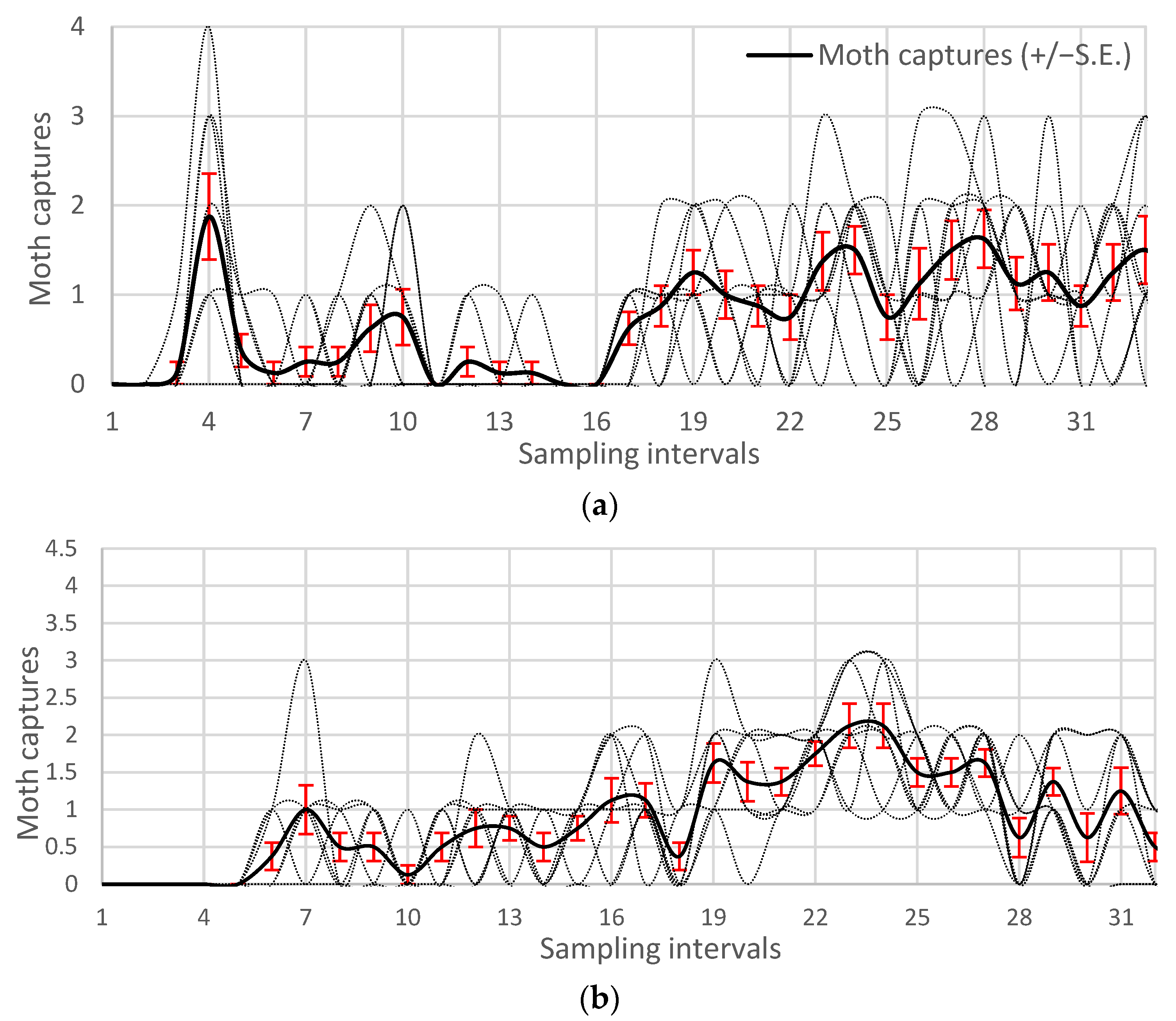
3.1. Moth Phenology and Population Density

During both observation years, 2021 and 2022, H. armigera had a consistent abundance throughout the dry bean growth season and completed three flights per year (Figure 1). Moth flights of spring moth emergence (1st flight) occurred in early to late May, while in most cases the 2nd flight started in June, peaked in July and was characterized by bimodal patterns. The 3rd flight was observed during the physiological maturation of bean production. This flight began in late August and lasted through early September, was characterized by consent moth observations but was quite abrupt. Due to this trend, the definition of discrete moth generations, especially for the third flight, proved quite challenging and especially in the cases where the number of moths captures was low. Therefore, we decided to pool the available data of each observation year for having an improved sampling space to generate the moth density for each H. armigera flight generation and estimate the related for each case bootstrapped pest risk thresholds (Figure 2).

The moth density of the first flight showed a clear moth peak representing the time where moth emergence is more likely to appear and without strong deviations from normality, while the second and especially the third flight, were characterized by multimodal patterns with strong deviations from normality. This was also the reason that we have decided to use straightforward non-parametric procedures to estimate the degree-day risk thresholds for H. armigera rather than estimating phenology metrics based on parametric distribution functions.

The description of moth capture data distribution frequencies, densities and quartiles for the first, second and third moth flight of H. armigera are shown in Figure 2. Despite the relatively large, for insects, data sets of all three flights were characterized by slight deviations from normality as it shown by the histograms, the density of moth captures as well as the relative boxplots.

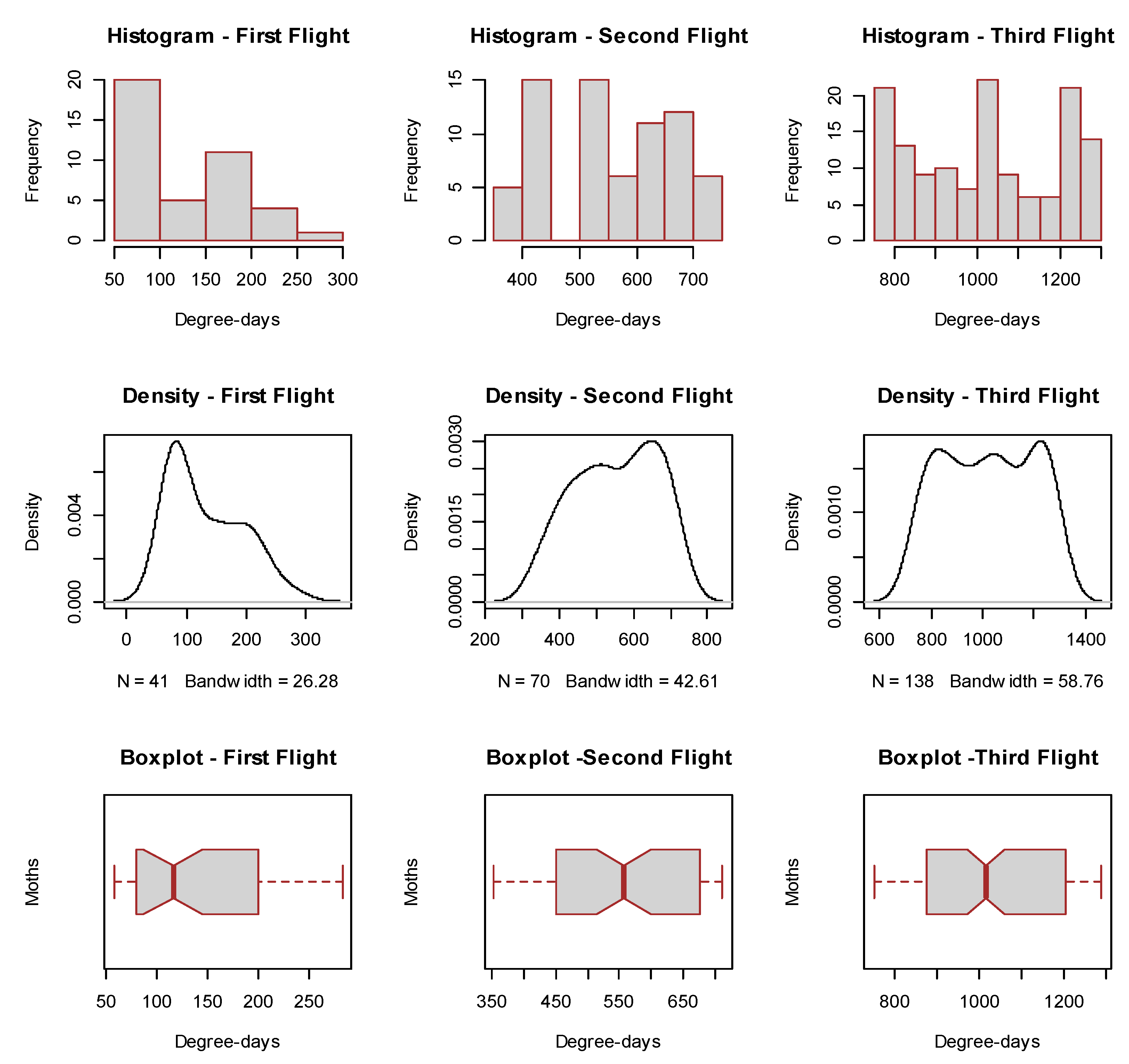
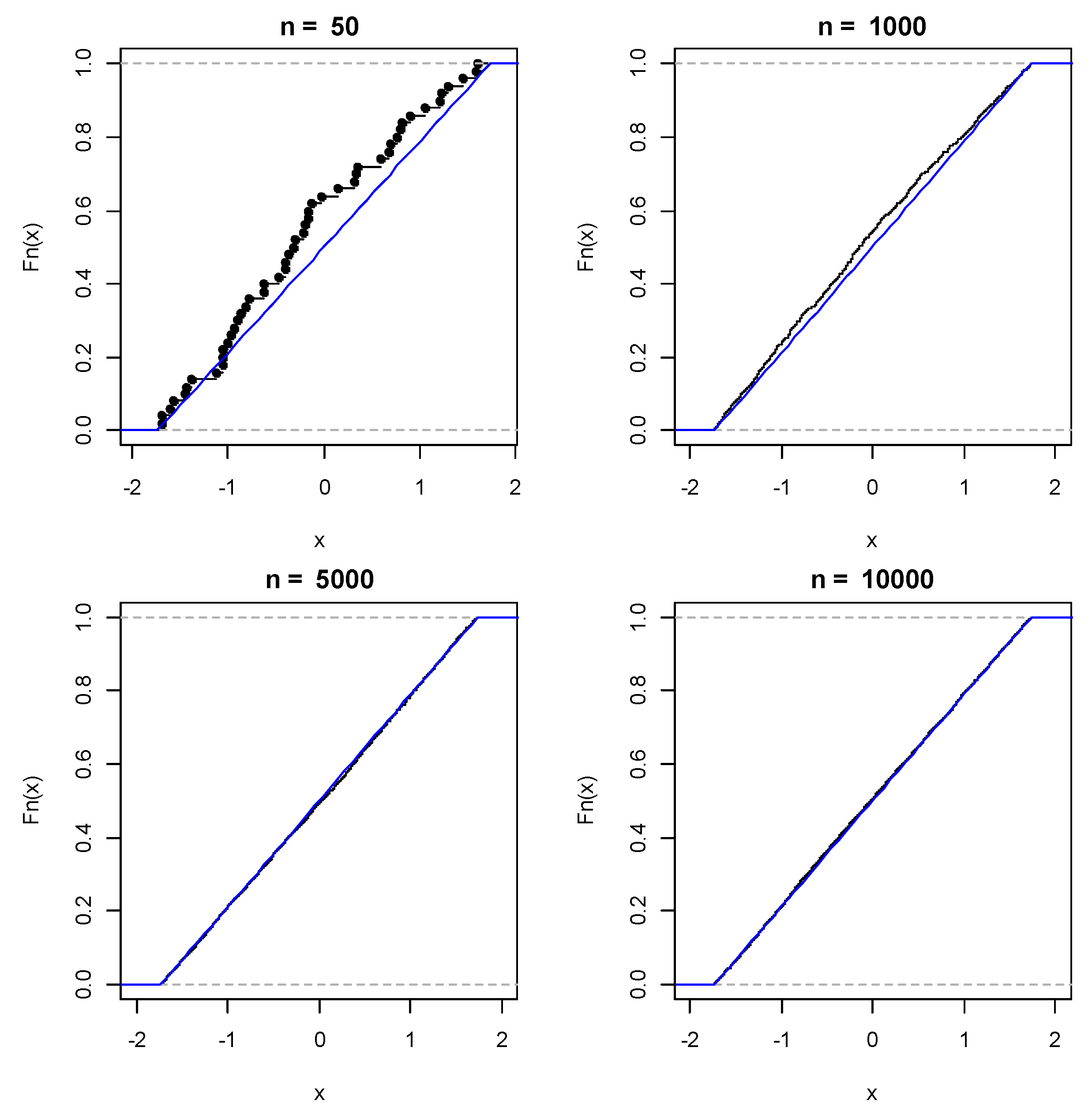
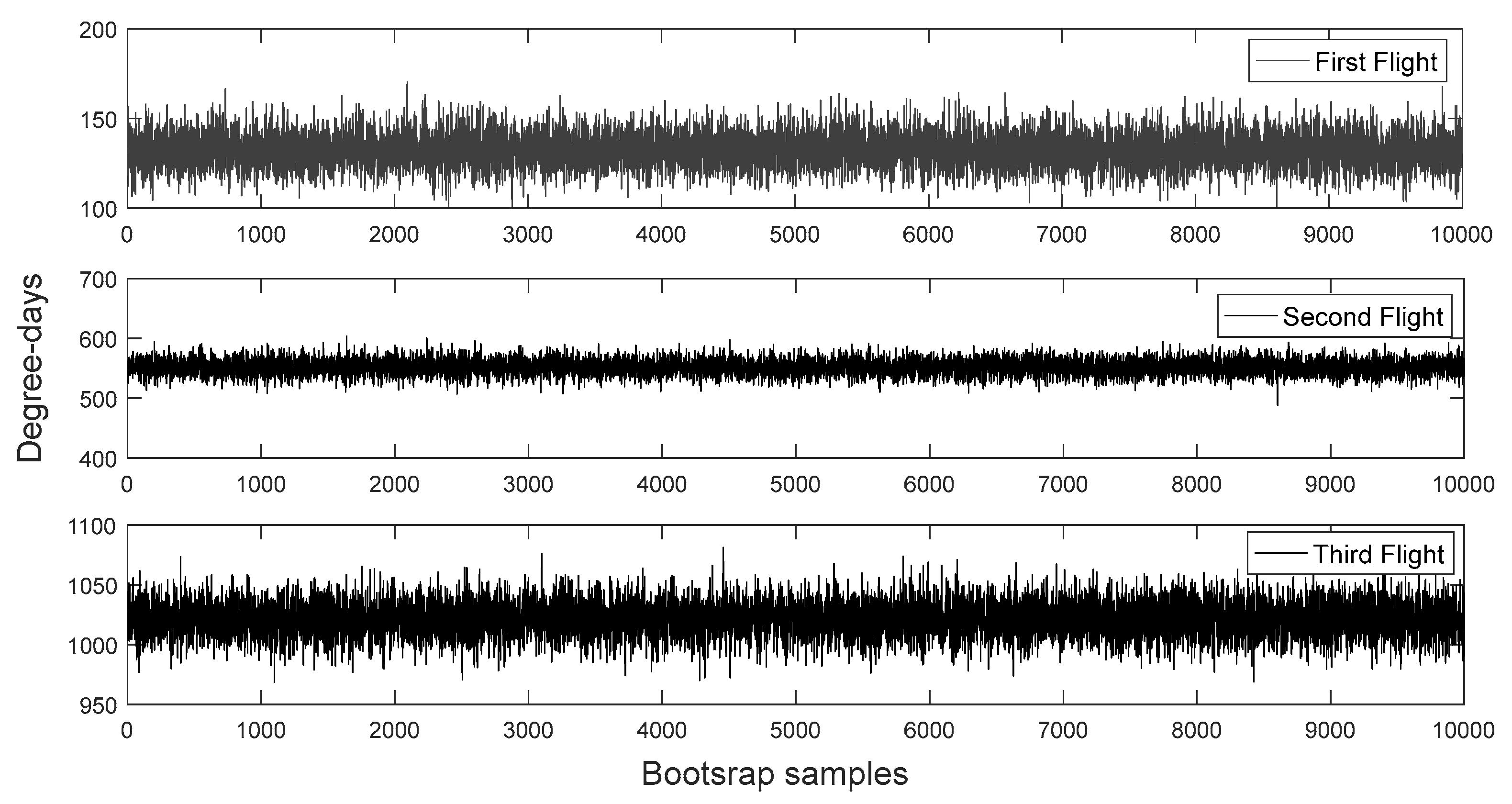
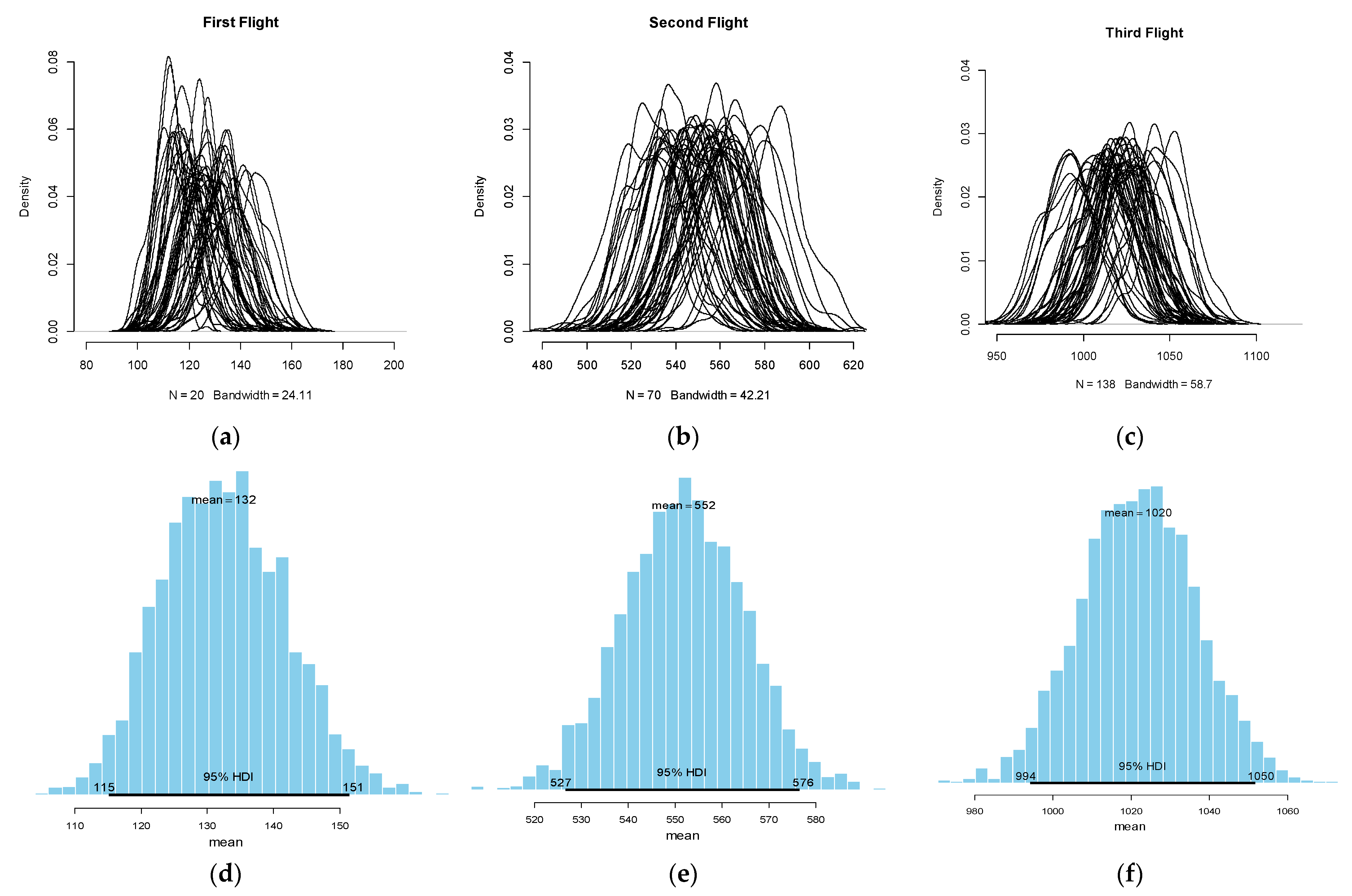
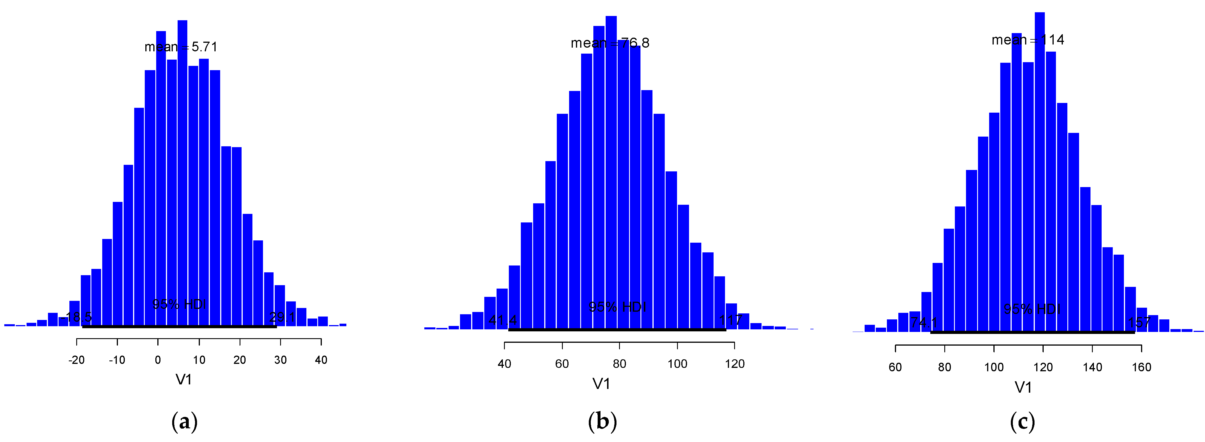
3.2. Bootstrapped Phenology and Bayesian Degree-Day Thresholds

The bootstrap procedure improved considerable the distribution of phenological data. The effect of different bootstrap sampling sizes n = 50, n = 100, n = 5000 and n = 10,000 on the sampling distribution of the first flight of H. armigera are shown in Figure 3. Importantly, as the bootstrap sample size increases, bootstrapping converges on the true sampling distribution for all three flights. Hence, increased bootstrap samples improved considerably the distribution patterns of H. armigera phenology although practically there was strong consistency of all estimates for n = 10,000 and afterwards. The simulation of 10,000 bootstrapped means of a random samples taken with replication from the vector of moth phenology for the first, second and third flight of H. armigera are shown in Figure 4.

The Bootstrap-simulated densities for the first, second and third flight generations of H. armigera are illustrated in Figure 5a–c and the respective to each moth flight posterior distributions, conditioned over the Dirichlet weights, are shown in Figure 5d–f. The highest number of H. armigera moth captures were observed at 132DD, while the subsequent second and third flights peaked at 552DDs and 1022DDs, respectively and according to the average method of heat summation. These values are the result of various combinations of simulated non-parametric Bayesian samples that collectively provide an estimate of the variability between random samples drawn from the same moth populations. The range of these potential samples allowed the procedure to construct confidence intervals and estimate the quantiles of moth population distributions (

Table 1. Degree-day risk thresholds and related phenological metrics for H. armigera flight generation according to the non-parametric Bayesian boostrap approach (n = 10,000 replications).

	Summary Statistics of the Posterior
Flight Generation	Draws	HDI *. Low	Mean	HDI. High	sd	Midrange
First (F1)	10,000	113.13	132.13	149.75	9.32	170
Second (F2)	10,000	527.78	551.72	579.27	13.2	531.9
Third (F3)	10,000	992.2	1021.6	1049.6	14.8	1020.3
	Quantiles and tendencies
	Q2.5%	Q25%	median	Q75%	Q97.5%	mode
First (F1)	114.04	125.76	131.83	138.21	150.96	79.4
Second (F2)	525.83	542.56	551.72	561.05	577.6	675.6
Third (F3)	992.7	1011.5	1021.56	1031.82	1050.09	1049.8

* HDI: High Density Intervals.

). Moreover, these values and especially, the mean or the median, consist of the pest risk thresholds since they are expressed in terms of physiological time and thus define the period of highest pest activity.

Moreover, based on the quantiles diagnostics we estimated the 2.5%, 50% and 97.5% percentiles of the median for each generation flight (Table 1). The quantiles consist of the requested degree-day risk thresholds since they represent the physiological time at which the peak in moth abundance is more likely to appear under field conditions. Based on the current analysis the first captures of a high density of H. armigera moths early in the season were observed at 114DD, peaked at 131DD and ended at 150DD. The second flight generation was observed at 525DD, peaked at 551DD and ended 577DD, whilst the third started at 992DD, peaked at 1021 and ended at 1050DD, respectively (Table 1). From a pest forecasting standpoint, these values consist of the basis of thermal time decision rules of the plant protection decision support.

The moth capture phenology data of the 2022 growth season were used to validate the pest risk thresholds. In most cases, the moth frequencies for each generation flight were very similar between the 2021 and 2022 growing years as shown by the posterior differences between the two data sets (Figure 6). Low difference indicates good fit between the proposed risk thresholds for 2021 and those observed in 2022. The slight deviations that were observed between predicted and observed phenology metrics should be attributed to the general appearance of H. armigera phenology which was characterized by a relatively low level of moth captures. This tendency was particularly higher for the third flight.

The posterior difference between the Bayesian degree—day thresholds developed with phenology data of 2021 and the observed with data of 2022 for the first flight generation of H. armigera were 5.71DD, which is remarkable low (Figure 6a). Thus, we can be fairly confident in choosing this threshold for predicting the appearance and peak of the first overwintering generation of H. armigera in the region of Prespa Lakes. Moreover, the degree-day thresholds posterior difference between 2021 and 2022 for the second flight generation is 77.8DD (Figure 6b). This difference can be characterized as being within acceptable levels given that during the summer it corresponds to a deviation of about 3 to 5 days. The posterior difference for the third flight generation of H. armigera was 114DD and was the highest compared to the two other flight generations (Figure 6c).

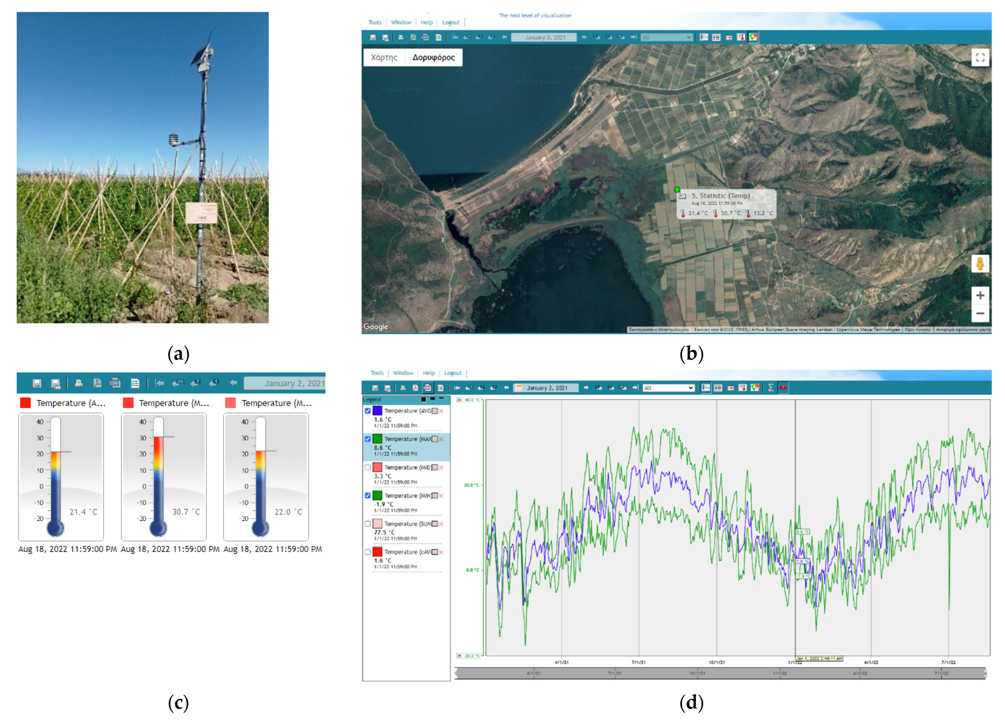
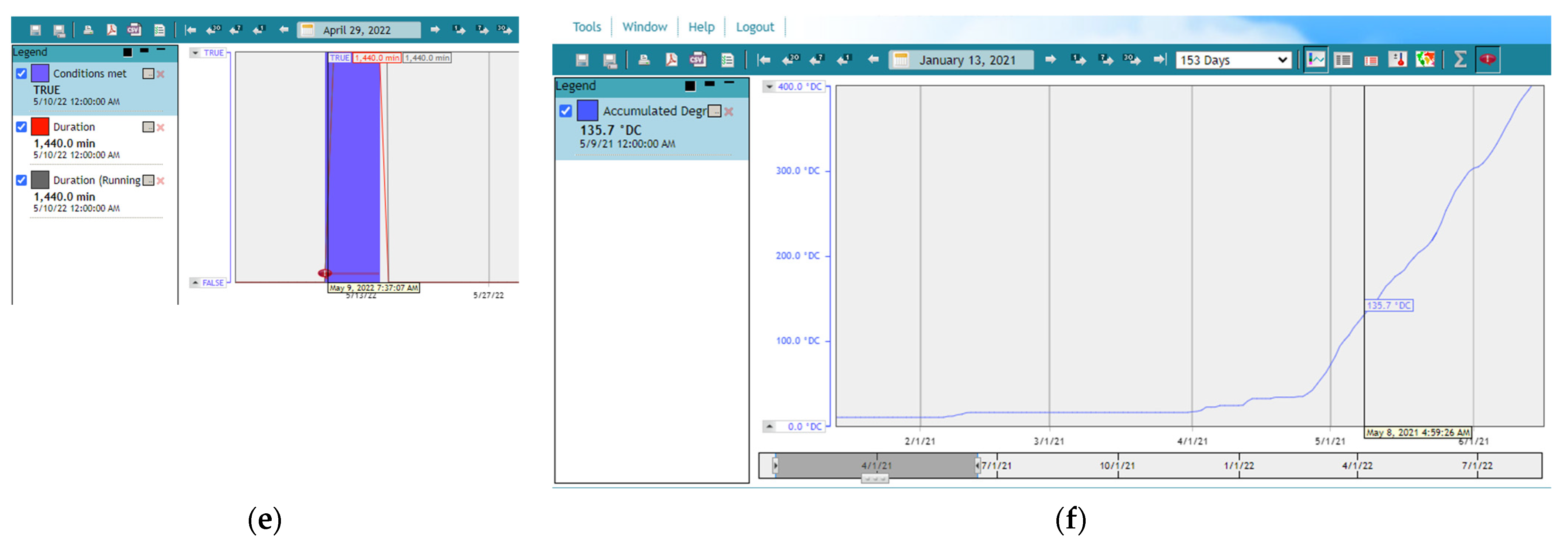
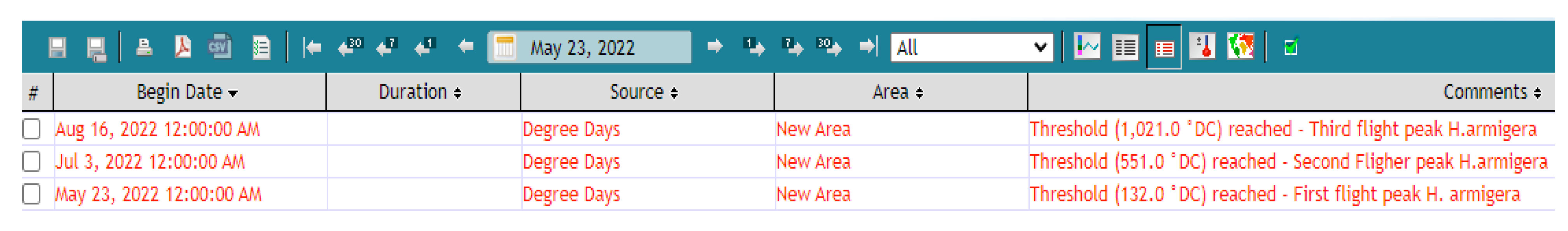
3.3. Decision Support System and H. armigera Forecasts

Figure 7a illustrates one of the meteorological weather stations (station code: deuterevon1) that were installed in the bean cultivation area of interest over the Prespa lakes in the prefecture of Florina. Figure 7b shows the location of the weather station based on the graphical user interface (GUI) of the digital plant protection decision support system. Figure 7c,d show the temperature indications and the respective heat summation recordings as illustrated in the graphical interface of the decision support system. Thus, overall, the implemented digital plant protection decision support system provides a variable information including the geolocation of the station through a google maps application, information of the weather sensors functioning as well as the illustration of real time weather recording i.e., mean, max and min temperatures, duration of risk thresholds and related accumulated degree-days) (Figure 7e,f). We have set as Biofix for heat recoding and related degree-days heat summation, the 1st of January. Temperature recordings that are higher than 9.42 °C, which is the lower developmental threshold of H. armigera, have been mostly recorded after the end of March for 2021 and the start of April for 2022.

The system creates alerts indicating the day and time period when the population activity of H. armigera is maximum by using the real-time weather data as input and the predefined pest risk threshold. (Figure 8). According to the generated alerts the first flight of H. armigera was predicted on 23 May, the second on 3 July and the third on 16 August. This is the most essential part of the plant protection decision support system since it can be used to initiate control methods. Apart from that, other information delivered by the decision support system through the meteorological network (not shown) is quite important for indicating the time period where the weather conditions are more favorable for crop development as well as pest increased activity and development.

4. Discussion

Quantifying and predicting pest phenology is a difficult task due to the inherent characteristics of abundance data which are collected under field conditions. For short and noisy data sets the estimation of the first and last events (i.e., moth emergence and end of generation) are very sensitive to changes in population abundance and often biased [54,55,56]. More data points might increase the probability of observing rare phenological events and estimate the parameters of the underlying distribution, but usually are not available in insect surveys.

In this work we present how robust phenological metrics for H. armigera in terms of degree-day heat summation thresholds can be obtained using non-parametric bootstrap methods. Particularly, we apply for the first time the Bayesian bootstrap, initially proposed by Rubin [51] as a Bayesian analogue of the Bootstrap proposed by Efron [48], to model phenology data of H. armigera and to develop degree-day risk thresholds. Although bootstrapping has become widely used in statistical analysis [57], there has been little reported concerning bootstrapped Bayesian analysis in phenology studies. Actually, to the best of our knowledge, there are no related studies which estimate essential phenology metrics of H. armigera in bean cultivation such as the time of its highest density.

It is important to note some conceptual variations between the Bayesian and the ordinal bootstrap. While the Bayesian bootstrap is probabilistic and assumes that the sample distribution is itself random and has a prior distribution, the ordinal bootstrap is a frequentist statistical technique that assumes that the sampling distribution is unknown but nonrandom [29,30,31,32]. According to the central limit theorem a high number of simulations yields to a reasonable approximation to the unknown normal population distribution and its parameters of interest. Placing a Dirichlet prior on the unknown distribution corresponds to Bayesian bootstrap [51]. The Bayesian perspective is more comprehensive to ordinal bootstrap since it produces no single value, but rather a whole probability distribution for the unknown parameter $\theta$ (e.g., moth peak) conditioned over the available phenology data (e.g., moth abundance). Thus, a conceptual standpoint of the Bayesian bootstrap, compared to traditional bootstrapping, is that the sampling distribution for the observations is multinomial and the prior for the weights is a limiting Dirichlet distribution. In simple terms the Dirichlet puts all its weight on the vertices of the simplex that correspond to the vectors of the bootstrapped probabilities of moth occurrence. This means that the proportion of times a data point occurs in the resampled moth data abundance set is proportional to that data points weighted according to the Dirichlet distribution.

Many applications of statistical models in entomological research require a vast amount of data to extract the parametric specifications of the probability distributions of interest that best describes insect phenology [58]. However, in most situations there will be insufficient data and prior information to justify such parametric assumptions [23]. The current work overcomes this problem proposing a non-parametric method as a flexible and robust tool to specify distributions of insects under field conditions and extract developmental parameters of interest. If, for instance, insect phenology is heavy tailed and/or explicit strong deviations from normality, and/or, a wrong family of distribution is chosen, this can lead to biased estimates of phenological events.

In this context, the current work is a different approach from most traditional ways of predicting moth dynamics having the advantage of accounting the non-parametric nature of phenology data. From an ecological standpoint, in the proposed Bayesian bootstrap approach, essential futures of the pest phenology patterns and the related distributions (i.e., central moments), can be ‘learned from the data’ rather than specified in advance from growth studies or by fitting parametric non-linear regression models. Moreover, since in poikilothermic organisms, such as arthropods and plants, the time evolution of phenological events is associated with changes in environmental temperature and the phenology metrics are generated on physiological time scale rather than calendar date. Thus, although we expect that the thermal requirements we have estimated for H. armigera to be constant, the dates of its highest density may change from year to year depending on the prevailing temperatures.

Concerning the number and duration of H. armigera generations, they depended upon the particular location of the research [59]. The time of the first generation of H. armigera was short, approximately 30 days in the field, and this is in accordance with other studies [60,61]. Moreover, in other regions of northern Greece H. armigera usually completes three generations per year as observed in the current study [61]. In Australia the pest completes at least three flights per year and catches in pheromone traps suggested a major peak in (male) numbers of H. punctigera in early spring [62]. In Israel, which is significantly warmer than Northern Greece, it has been observed that the post diapause adult emergence of H. armigera begins in late April, and 50% of females enclose before 6 May, which is 9 days before 50% of the males do [63], while in central Japan, which is much colder, H. armigera moths emerge in early June [64].

In this work the prediction for the overwintering generation peak is 132DD a value which generally is in accordance with studies conducted in cotton cultivations where adult emergence occurred usually between early and late May [61]. In other locations and where information is available, such in the southeast of Caspian, the adults appeared above 219DD, but temperature recordings were based on remote sensing [65]. Moreover, there were no considerable differences of the first flight of H. armigera in early spring as observed in 2021 and 2022. However, we observed deviations of about 70–100DDs, between the years 2021 and 2022, for the second and third flights, respectively. These deviations were indeed to be expected, considering that phenology data after the first and especially second moth flights, are noisy and characterized by multimodal patterns. This is a general trend, observed also in other moth studies and justified, to some extent, by the fact that, as temperatures are favorable for growth, populations increase causing an overlapping of generations [20,46]. In addition, harvesting crops with a shorter biological cycle in nearby areas may cause moths to move to the longer-lived bean cultivation in order to secure food for their subsistence and blurring the in-cultivation phenology patterns. Yet, there are no related works that focus on dry bean cultivation and that provide information for all flight generations of H. armigera to be compared with. Therefore, degree-day risk thresholds as estimated in this work for all three generations is very important since bean cultivation is exposed to the attack not only of the first flight generation but also of the succeeding.

However, despite the practical utility of the current degree-day thresholds some limitations of the modeling approach should be also noted. For instance, the bootstrap method does not improve point estimate, meaning the quality of bootstrapping depends on the quality of collected data and the assumptions being made when undertaking the analysis [48]. Therefore, any field experimentation should be a good approximation of the whole population data to get robust phenology metrics. One other disadvantage, as well as of any degree-days modeling approach, is that apart of the thermal environment it does not account on other factors that might affect pest occurrence. For example, when a population experiencing unmeasured changes in abundance such as predation [66] and/or interspecies competition [67], it becomes quite challenging to determine whether moth changes, especially the first and last observations, are a consequence of changes in actual phenology, or changes in population abundance. Migration and host range might be an additional factor affecting moth abundance and phenology. The species can migrate over long distances (>100 km) and aided by wind up to 2000 km [68], while the ability for long distance movements of seasonal migration from low to higher latitudes in summer, usually on warm winds preceding cold fronts, is a characteristic of H. armigera [69].

Nevertheless, in the current work we have observed a consistent presence of the pest in all experimental fields and during both study years, supplying evidence that probably a local population of H. armigera has been established in the region of Prespa Lakes in northern Greece. Additionally, despite the factors affecting H. armigera abundance environmental temperature is the predominate factor affecting its bio-ecology and related phenology patterns [70]. It is known, for example, that abrupt changes in phenology and population number of H. armigera occurred after abrupt temperature changes, while climate change had a greater effect on the phenology of H. armigera at higher latitudes than at lower latitudes and led to a greater increase in population size at lower latitudes than at higher latitudes [71].

Despite any inherent ecological constrains that might affect insect abundance, temperature is by far the most predominant factor and therefore, the current work provides useful information for rational management of H. armigera. Moreover, our study provides an alternative to parametric modeling approach for handling insect occurrence data and extract vital phenology metrics. The Bayesian bootstrap particularly is powerful statistical technique for posterior simulation especially working with small sample sizes (i.e., <40) that cannot be handled by assuming a normal distribution [67,72,73,74]. From a pest management standpoint, the study demonstrates the importance of the developed pest risk thresholds for the development and operation of real time decision support systems for pest management. Currently, we are looking forward to improve H. armigera forecasts and expand the functionality of the decision support system by including more pest threats and validate its functionality into more areas.

Finally, the developed pest risk thresholds will be integrated into VELOS, a novel cloud based smart ecosystem for precise farming and pest management of bean farms [75]. VELOS leverages Information and Communication Technologies such as Internet of Things, Artificial Intelligence, Big Data analytics, and Unmanned Aerial/Ground Vehicles for extracting knowledge in order to provide an integrated solution to effectively support decision-making, efficiently managing pesticide application and its scheduling. The pest risk threshold subsystem of VELOS will drive the activation of other VELOS subsystems (e.g., UAVs and UGVs), while it will constitute a verification of the output of the pest damage detection engine subsystem.

5. Conclusions

In the current study we applied non-parametric Bayesian bootstrap methods for estimating problematic metrics of phenology patterns such as the moth peak emergence and onset of successive generations of H. armigera. Conceptually, and without going into deep mathematical details, the approach allows to estimate parameters of the unknown distribution of moth phenology data and adapted in terms of physiological time and without being restricted to a family of predefined distributions such as the normal, Weibull etc.

Additionally, the approach resulted in the development of degree-day thresholds to be used as a rational tool for predicting the most important phenological events of H. armigera including start, peak and end of each generation. Although, these thresholds have been incorporated into digital plant protection systems their implementation should always include the consideration of their consistence in terms of improving their performance.

Despite the inherent limitation of the current study, we expect that the present study fills the gap of the absence of non-parametric approaches in analyzing insect phenological patterns. Furthermore, it proposes degree-day thresholds utile for predicting occurrence of H. armigera in bean cultivation and that are necessary to develop digital plant protection systems for rational management of H. armigera and reduce the hazardous of synthetic chemicals.

References

1. Parde, V.D.; Sharma, H.C.; Kachole, M.S. Protease Inhibitors in Wild Relatives of Pigeonpea against the Cotton Bollworm/Legume Pod Borer, Helicoverpa armigera. Am. J. Plant Sci. 2001, 3, 70–72. [Google Scholar]
2. Zalucki, M.P.; Daglish, G.; Firempong, S.; Twine, P.H. The biology and ecology of Heliothis armigera (Hubner) and H. punctigera Wallengren (Lepidoptera: Noctuidae) in Australia: What do we Know? Aust. J. Zool. 1986, 34, 779–814. [Google Scholar] [CrossRef]
3. Sharma, H.C. Heliothis/Helicoverpa Management: Emerging Trends and Strategies for Future Research; Oxford and IBH Publishing Co., Pvt. Ltd.: New Delhi, India, 2005; p. 469. [Google Scholar]
4. Smith, I.M.; McNamara, D.G.; Scott, P.R.; Holderness, M. Quarantine Pests for Europe; CAB International: Wallingford, UK, 1997. [Google Scholar]
5. Damos, P. Current issues in integrated pest management of Lepidoptera pest threats in Industrial crop models. In Lepidoptera: Ecology, Behavior and Management; Guerritore, E., DeSare, J., Eds.; NovaScience: New York, NY, USA, 2012; ISBN 978-1-62417-249-6. [Google Scholar]
6. Fitt, G.P. The ecology of Heliothis species in relation toagro-ecosystems. Ann. Rev. Entomol. 1989, 34, 17–52. [Google Scholar] [CrossRef]
7. Damos, P.; Tsikos, E.; Louta, M.; Papathanasiou, F. Towards the Development of a Smart Plant Protection Solution for Improved Pest Management of Dry Beans (Phaseolus vulgaris L.) in Northern Greece. In Proceedings of the 1st International Electronic Conference on Entomology, Basel, Switzerland, 1–15 July 2021. [Google Scholar] [CrossRef]
8. Papadopoulos, I.; Papathanasiou, F.; Vakali, C.; Kazoglou, I.; Tamoutsidis, E. Local landraces of dry beans (Phaseolus vulgaris L.): A valuable resource for organic production in Greece. Acta Hortic. 2012, 933, 75–81. [Google Scholar] [CrossRef]
9. Papathanasiou, F.; Barbayiorgis, A.; Papadopoulou, V.; Kareklas, E.; Galaitsis, D.; Papadopoulou, F.; Tamoutsidis, E.; Papadopoulos, I. Physiological performance and yield of dry bean (Phaseolus vulgaris L.) genotypes under water deficit. In Proceedings of the Book of Abstracts of the AgriBalkan-Balkan Agricultural Congress, Edirne, Turkey, 8–11 September 2014; p. 398. [Google Scholar]
10. Zalucki, M.P. Heliothis: Research Methods and Prospects; Springer: Berlin/Heidelberg, Germany, 1991. [Google Scholar]
11. Carvalho, F.P. Pecticides, environment and food safety. Food Energy Secur. 2017, 6, 48–60. [Google Scholar] [CrossRef]
12. Pal, S.; Chatterjee, H.; Senapati, S.K. Monitoring of Helicoverpa armigera using pheromone traps and relationship of moth activity with larval infestation on Carnation (Dianthus caryophyllus) in Darjeeling Hills. J. Entomol. Res. 2014, 38, 23–26. [Google Scholar]
13. Kumar Sharma, P.; Kumar, U.; Vyas, S.; Sharma, S.; Shrivastava, S. Monitoring of Helicoverpa armigera (Hübner) (Lepidoptera: Noctuidae) Through Pheromone Traps In Chickpea (Cicer arietinum) Crop and influence of Some abiotic factors on insect population. IOSR J. Environ. Sci. Toxicol. Food Technol. (IOSR-JESTFT) 2012, 1, 44–46. [Google Scholar] [CrossRef]
14. McGeachie, W. The effects of moonlight illuminance, temperature and wind speed on light-trap catches of moths. Bull. Entmol. Res. 1989, 79, 185–192. [Google Scholar] [CrossRef]
15. Choi, S.W. The effects of weather factors on the abundance and diversity of moths in a temperate deciduous mixed forest of Korea. Zool. Sci. 2018, 25, 53–58. [Google Scholar] [CrossRef]
16. Nibouche, S.; Gozé, E.; Babin, R.; Beyo, J.; Brévault, T. Modeling Helicoverpa armigera (Hübner) (Lepidoptera: Noctuidae) damages on cotton. Environ. Entomol. 2007, 36, 151–156. [Google Scholar] [CrossRef] [Green Version]
17. Dalal, P.K.; Arora, R. Model-based phenology prediction of Helicoverpa armigera (Hübner) (Noctuidae: Lepidoptera) on tomato crop. J. Plant Dis. Prot. 2019, 126, 281–291. [Google Scholar] [CrossRef]
18. Jallow, F.A.M.; Masaya, M. Infuence of temperature on the rate of development of Helicoverpa armigera (Hübner) (Lepidoptera: Noctuidae). Appl. Entomol. Zool. 2001, 36, 427–430. [Google Scholar] [CrossRef] [Green Version]
19. Amer, A.E.A.; El-Sayed, A. Effect of different host plants and artificial diet on Helicoverpa armigera (Hübner) (Lepidoptera: Noctuidae) development and growth index. J. Entomol. 2014, 11, 299–305. [Google Scholar] [CrossRef] [Green Version]
20. Damos, P.; Savopoulou-Soultani, M. Temperature driven models for Insect development and Vital Thermal Requirements. Psyche 2012, 2012, 123405. [Google Scholar] [CrossRef] [Green Version]
21. Damos, P.; Karabatakis, S. Real time pest modeling trhough the world wide web: Decision making from theory to praxis. IOBC-WPRS Bull. 2013, 91, 253–258. [Google Scholar]
22. Edwars, C.; Crone, E.E. Fitting phenological curves with GLMMs. Oikos 2022, 130, 1335–1345. [Google Scholar]
23. Damos, P. A stepwise algorithm to detect significant time lags in ecological time series in terms of autocorrelation functions and ARMA model optimisation of pest population seasonal outbreaks. Stoch. Environ. Res. Risk Assess. 2016, 30, 1961–1980. [Google Scholar] [CrossRef]
24. Munholland, P.L.; Kalbfleish, J.D.; Dennis, B. A stochastic model for insect life history data. In Estimating and Analysis of Insect Populations. Lecture Notes in Statistics; McDonald, L.L., Manly, B.F.L., Lochwood, J.A., Logan, J.A., Eds.; Springer: New York, NY, USA, 1988; Volume 55. [Google Scholar]
25. Maurer, J.A.; Shepard, J.H.; Crabo, L.G.; Hammond, P.C.; Zack, R.S.; Peterson, M.A. Phenological responses of 215 moth species to interannual climate variation in the Pacific Northwest from 1895 through 2013. PLoS ONE. 2018, 13, e0202850. [Google Scholar] [CrossRef] [PubMed]
26. Damos, P.; Soulopoulou, P. Do Insect Populations Die at Constant Rates as They Become Older? Contrasting Demographic Failure Kinetics with Respect to Temperature According to the Weibull Model. PLoS ONE 2015, 10, e0127328. [Google Scholar]
27. Moussus, J.P.; Jiquet, J.F. Featuring phenological estimators using simulated data. Methods Ecol. Evol. 2010, 1, 140–150. [Google Scholar] [CrossRef]
28. Damos, P. Demography and randomized life table statistics for the peach twig borer Anarsia lineatella (Lepidoptera: Gelechiidae). J. Econ. Entomol. 2013, 106, 675–682. [Google Scholar] [CrossRef] [PubMed]
29. Gershman, S.J.; Blei, D.M. A tutorial on Bayesian nonparametric models. J. Math. Psychol. 2012, 56, 1–12. [Google Scholar] [CrossRef] [Green Version]
30. Shao, J.; Tu, D. Bayesoan bootrsrap and random weighting. In The Jacknife and Bootrsap. Springer Series in Statistics; Springer: New York, NY, USA, 1995. [Google Scholar]
31. Muliere, P.; Secchi, P. Bayesian nonparametric inference and boostrap techniques. Ann. Inst. Stat. Math. 1996, 48, 663–673. [Google Scholar] [CrossRef]
32. Galvani, M.; Bardelli, C.; Figini, S.; Muliere, P. A Bayesian Nonparametric Learning Approach to Ensemble Models Using the Proper Bayesian Bootstrap. Algorithms 2021, 14, 11. [Google Scholar] [CrossRef]
33. Ellison, A.M. Bayesian inference in ecology. Ecol. Lett. 2004, 7, 509–520. [Google Scholar] [CrossRef]
34. Morevie, M.A.; Davison, A.C.; Pasquier, D.; Charmillot, P.J. Bayesian forecasting of grape moth emergence. Ecol. Mod. 2006, 197, 478–489. [Google Scholar] [CrossRef]
35. Wesner, J.S.; Pomeranz, J.P.F. Choosing priors in Bayesian ecological models by simulating from the prior predictive distribution. Ecosphere 2021, 12, e03739. [Google Scholar] [CrossRef]
36. Sanbasivan, R.; Das, S.; Sahu, S.K. A Bayesian perspective of statistical machine learning for big data. Comput. Stat. 2020, 35, 893–930. [Google Scholar] [CrossRef] [Green Version]
37. Singh, N.; Gupta, N. Bayesian network for decision-support on pest management of tomato fruit borer, H. armigera. Int. J. Eng. Technol. 2017, 6, 168–170. [Google Scholar] [CrossRef] [Green Version]
38. Apel, H.; Herrmann, A.; Richter, O. A decision support system for integrated pest managment of Helicoverpa armigera in the tropics and subtropics by means of a rule-based Fuzzy model. Z. Fur Agrainformatik 1999, 7, 83–90. [Google Scholar]
39. Narava, R.; Sai Ram Kumar, D.V.; Jaba, J.; Kumar, A.P.; Rao, R.G.V.; Rao, S.R.; Mishra, S.P.; Kukanur, V. Development of Temporal Model for Forecasting of Helicoverpa armigera (Noctuidae: Lepidopetra) Using Arima and Artificial Neural Networks. J. Insect Sci. 2022, 22, 2. [Google Scholar] [CrossRef] [PubMed]
40. Nanushi, O.; Sitokonstantinou, V.; Tsoumas, I.; Konteos, C. Pest presence prediction using interpretable machine learning. arXiv 2022, arXiv:2205.07723. [Google Scholar]
41. Almalki, F.A.; Soufiene, B.O.; Alsamhi, S.H.; Sakli, H. A Low-Cost Platform for Environmental Smart Farming Monitoring System Based on IoT and UAVs. Sustainability 2021, 13, 5908. [Google Scholar] [CrossRef]
42. Xu, M.; David, J.M.; Kim, S.H. The fourth industrial revolution: Opportunities and challenges. Int. J. Financ. Res. 2018, 9, 90–95. [Google Scholar] [CrossRef] [Green Version]
43. Tinte, M.M.; Chele, K.H.; van der Hooft, J.J.J.; Tugizimana, F. Metabolomics-Guided Elucidation of Plant Abiotic Stress Responses in the 4IR Era: An Overview. Metabolites 2021, 11, 445. [Google Scholar] [CrossRef]
44. Barteková, A.; Praslička, J. The effect of ambient temperature on the development of cotton bollworm (Helicoverpa armigera Hübner, 1808). Plant Prot. Sci. 2006, 42, 135–138. [Google Scholar] [CrossRef]
45. Mironidis, G.K.; Savopoulou-Soultani, M. Development, Survivorship and Reproduction of Helicoverpa armigera (Lepidoptera: Noctuidae) Under Constant and Alternating Temperatures. Environ. Entomol. 2008, 37, 16–28. [Google Scholar] [CrossRef]
46. Damos, P.T.; Savopoulou-Soultani, M. Development and statistical evaluation of models in forecasting moth phenology of major lepidopterous peach pest complex for Integrated Pest Management programs. Crop Prot. 2010, 29, 1190–1199. [Google Scholar] [CrossRef]
47. Chernick, M.R. Boostrap Methods: A Practitioner’s Guide (Wiley Series in Probability and Statistics), 1st ed.; Wiley-Interscience: New York, NY, USA, 2007. [Google Scholar]
48. Efron, B. The Jackknife, the Bootstrap and Other Resampling Plans; Society for Industrial and Applied Mathematics: Philadelphia, PA, USA, 1982. [Google Scholar]
49. Efron, B.; Tibshirani, R. Software (Bootstrap, Cross-Validation, Jackknife) and Data for the Book “An Introduction to the Bootstrap”, In Package Bootrstap; Chapman and Hall: London, UK, 1993. [Google Scholar]
50. Alfaro, M.E.; Zoller, S.; Lutzoni, F. Bayes or boostrap? A simulation study comparing the performance of Bayesian Markov chain Monte Carlo sampling and bootstrapping in assessing phylogenetic confidence. Mol. Biol. Evol. 2003, 20, 255–266. [Google Scholar] [CrossRef] [Green Version]
51. Rubin, D.B. The bayesian boostrap. Ann. Stat. 1981, 9, 130–134. [Google Scholar] [CrossRef]
52. Calatayud, J.; Jornet, M.; Mateu, J. A stochastic Bayesian bootstrapping model for COVID-19 data. Stoch. Environ. Res. Risk Assess. 2022, 36, 2907–2917. [Google Scholar] [CrossRef] [PubMed]
53. Dirichletprocess Package Dirichletprocess: An R Package for Fitting Complex Bayesian Nonparametric Models. Available online: https://cran.r-project.org/web/packages/dirichletprocess/vignettes/dirichletprocess.pdf (accessed on 10 August 2022).
54. van Strien, A.J.; Plantenga, W.F.; Sodaat, L.L.; van Swaay, C.A.M.; WallisDeVries, M.F. Bias in phenology assessments based on first appearance data of butterlies. Oecologia 2008, 156, 227–235. [Google Scholar] [CrossRef]
55. Miller-Rushing, J.A.; Inouye, D.W.; Primack, R.B. How well do first flowering dates measure plant responses to climate change? The effects of population size and sampling frequency. J. Ecol. 2008, 96, 1289–1296. [Google Scholar]
56. Inouye, B.D.; Ehrlén, J.; Undeewoos, N. Phenology as a process rather than an event: From individual reaction norms to community metrics. Ecol. Monog. 2019, 89, e01352. [Google Scholar] [CrossRef]
57. Steward, T.J. Experience with a Byesian bootstrap method incorporating proper prior information. Commun. Stat. Theory Meth. 1986, 15, 3205–3225. [Google Scholar] [CrossRef]
58. Damos, P.; Bonsignore, C.P.; Gardi, F.; Avtzis, D.N. Phenological responses and a comperative phylogenetic insight of Anarsia lineatella and Grapholita molesta between distinct geographical regions within the Mediterranean basin. J. Appl. Entomol. 2014, 138, 528–538. [Google Scholar] [CrossRef]
59. EPPO/CABI. European and Mediterranean Plant Protection Organization/CAB International. Helicoverpa armigera. In Quarantine Pests for Europe, 2nd ed.; Smith, I.M., McNamara, D.G., Scott, P.R., Holderness, M., Eds.; CAB International: Wallingford, UK, 1997; pp. 289–294. [Google Scholar]
60. Damos, P.; Mantzoukas, S.; Theoharis, X.; Zaggos, G.; Staurakoulis, N.; Karanastasi, E.; Perdikis, D. Development and first evaluation of seasonal and spatial models of Helicoverpa armigera and Tuta absoluta in industrial tomato cultivations in the prefectures of Ilia and Achaia. In Proceedings of the 16th PanHellenic Conference on Entomology, Heraklion, Greece, 20–30 October 2015. [Google Scholar]
61. Mironidis, G.K.; Stamopoulos, D.C.; Savopoulou-Soultani, M. Overwintering survival and spring emergence of Helicoverpa armigera (Lepidoptera: Noctuidae) in northern Greece. Environ. Entomol. 2010, 39, 1068–1084. [Google Scholar] [CrossRef]
62. Baker, G.H.; Tann, C.R.; Fitt, G.P. A tale of two trapping methods: Helicoverpa spp. (Lepidoptera, Noctuidae) in pheromone and light traps in Australian cotton production systems. Bull. Entomol. Res. 2011, 101, 9–23. [Google Scholar] [CrossRef]
63. Zhou, X.; Applebaum, S.W.; Coll, M. Overwintering and spring migration in the bollworm Helicoverpa armigera (Lepidoptera: Noctuidae) in Israel. Environ. Entomol. 2000, 29, 1289–1294. [Google Scholar] [CrossRef]
64. Qureshi, M.H.; Murai, T.; Yoshida, H.; Shiraga, T.; Tsumuki, H. Population variation in diapause induction and termination of Helicoverpa armigera (Lepideptera: Noctuidae). Appl. Entomol. Zool. 2000, 35, 357–360. [Google Scholar] [CrossRef]
65. Jokar, M. A thermal forecasting model for the overwintering generation of cotton bollworm by remote sensing in the southeast of Caspian Sea. Span. J. Agric. Res. 2022, 20, e1001. [Google Scholar] [CrossRef]
66. Liu, B.; Yang, L.; Yang, F.; Wang, Q.; Yang, Y.Z.; Lu, Y.H.; Gardiner, M.M. Landscape diversity enhances parasitism of cotton bollworm (Helicoverpa armigera) eggs by Trichogramma chilonis in cotton. Biol. Control. 2016, 93, 15–23. [Google Scholar] [CrossRef]
67. Bheemanna, M.; Ashoka, J.; Wali, V.; Dave, S.; Bheemanna, M.; Ashoka, J.; Shivayogiyappa, P.; Lim, K.S.; Chapman, J.W.; Sane, S.P. Evidence for facultative migratory flight behavior in Helicoverpa armigera (Noctuidae: Lepidoptera) in India. PLoS ONE 2021, 16, e0245665. [Google Scholar]
68. Behere, G.T.; Tay, W.T.; Russell, D.A.; Kranthi, K.R.; Batterham, P. Population genetic structure of the cotton bollworm Helicoverpa armigera (Hübner) (Lepidoptera: Noctuidae) in India as inferred from EPIC-PCR DNA markers. PLoS ONE 2013, 8, e53448. [Google Scholar] [CrossRef] [PubMed] [Green Version]
69. Feng, H.Q.; Wu, K.M.; Ni, Y.X.; Cheng, D.F.; Guo, Y.Y. High-Altitude Windborne Transport of Helicoverpa armigera (Lepidoptera: Noctuidae) in Mid-Summer in Northern China. J Insect Behav 2005, 18, 335–349. [Google Scholar] [CrossRef]
70. Aheer, G.M.; Ali, A.; Akram, M. Effect of weather factors on populations of Helicoverpa armigera moths at cotton-based agro-ecological sites. Entomol. Res. 2009, 29, 36–42. [Google Scholar] [CrossRef]
71. Huang, J. Effects of climate change on different geographical populations of the cotton bollworm Helicoverpa armigera (Lepidoptera, Noctuidae). Ecol. Evol. 2021, 11, 18357–18368. [Google Scholar] [CrossRef]
72. Rousselet, G.A.; Pernet, C.R.; Wilcox, R.R. The percentile Bootstrap: A primer with step-by-step instructions in R. Adv. Meth. Pract. Psych. Sci. 2021, 4, 2515245920911881. [Google Scholar] [CrossRef]
73. Bååth, R. The Non-Parametric Bootstrap as a Bayesian Model. Publishable Stuff. Available online: http://www.sumsar.net/ blog/2015/04/the-non-parametric-bootstrap-as-a-bayesianmodel/ (accessed on 18 April 2015).
74. Canty, A.; Ripley, B.D. Boot: Bootstrap Functions, Version 1.3-25; Comprehensive R Archive Network. Available online: https://CRAN.R-project.org/package=boot (accessed on 5 August 2022).
75. Louta, M.; Papathanasiou, F.; Damos, P.; PLoSkas, N.; Dasygenis, M.; Kyriakidis, T.; Dimokas, N.; Balafas, V.; Chatzisavvas, A.; Karampelia, I.; et al. Intelligent pesticide and irrigation management in precision agriculture: The case of VELOS project. HAICTA. In Proceedings of the 10th International Conference on ICT in Agriculture, Food & Environment, Athens, Greece, 22–25 September 2022. [Google Scholar]
Figure 1. Seasonal flight patterns of H. armigera (black line) as observed with eight pheromone traps (dashed lines) placed in four experimental dry bean fields in the Prespa region of Northern Greece. Sampling intervals are 3-day observations starting from mid-April till end of August 2021 (a) and 2022 (b).
Agronomy 12 02474 g001
Figure 2. Description of moth capture data distribution frequencies, densities and empirical quartiles for the first, second and third flight of H. armigera moths in respect to accumulated degree-days > 10.1 °C after 1 January 2021.
Agronomy 12 02474 g002
Figure 3. The effect of different bootstrap sampling sizes n = 50, n = 100, n = 5000 and n = 10,000 on the sampling distribution of H. armigera first flight.
Agronomy 12 02474 g003
Figure 4. Simulation of a sample of n = 10,000 bootstrapped means,   θ ^ 1 * , , θ ^ 10,000 * , of random samples taken with replication from the vector of moth phenology for the first, second and third flight of H. armigera.
Agronomy 12 02474 g004
Figure 5. Some simulated bootstrapped densities (n = 50), for the first (a), second (b) and third (c) flight generations of H. armigera. Posterior frequency distributions according to the Bayesian bootstrap procedure (n = 10,000) for the first (d), second (e) and third flight (f) of H. armigera. Means represent the degree-days of the highest pest activity (i.e., peak in moth abundance) and HDI the related 95% high density intervals.
Agronomy 12 02474 g005
Figure 6. Posterior difference (V1) according to the Bayesian bootstrap procedure (n = 10,000) between predicted (2021) and observed degree-day risk thresholds (2022) expressed in terms of heat summations (i.e., peak in moth abundance) and the related 95% high density intervals (HDI), for the first (a), second (b) and third flight (c) of H. armigera.
Agronomy 12 02474 g006
Figure 7. A representative meteorological station (a) and its location in the Prespa lake area in the prefecture of Florina (b). Graphical User Interface (GUI) and real time software outputs of: mean, max and min temperature online sensor indications (c), mean (blue), max and min (green) daily temperature recordings (1 January 2021 so far) (d), pest risk thresholds indications and their duration for the first flight of H. armigera (e) and accumulated degree-days from 1 January 2021 (f).
Agronomy 12 02474 g007aAgronomy 12 02474 g007b
Figure 8. GUI event list output and the real time H. armigera thermal risk thresholds generated by Adcon® telemetry software plant protection decision support system used in the current study. Note that the default software output of 1,021.0 DC corresponds to 1021 accumulated DDs and so on.
Agronomy 12 02474 g008