Article

New Approaches for the Assimilation of LAI Measurements into a Crop Model Ensemble to Improve Wheat Biomass Estimations

1
Crop Science Research Group, Institute of Crop Science and Resource Conservation, University of Bonn, Katzenburgweg 5, 53115 Bonn, Germany
2
Agrosphere (IBG-3), Institute of Bio- and Geosciences, Forschungszentrum Jülich, 52425 Jülich, Germany
3
xarvioTM BASF Digital Farming GmbH, Im Zollhafen 24, 50678 Köln, Germany
*
Author to whom correspondence should be addressed.
Agronomy 2020, 10(3), 446; https://doi.org/10.3390/agronomy10030446
Submission received: 29 January 2020 / Revised: 13 March 2020 / Accepted: 21 March 2020 / Published: 24 March 2020

Abstract

:
The assimilation of LAI measurements, repeatedly taken at sub-field level, into dynamic crop simulation models could provide valuable information for precision farming applications. Commonly used updating methods such as the Ensemble Kalman Filter (EnKF) rely on an ensemble of model runs to update a limited set of state variables every time a new observation becomes available. This threatens the model’s integrity, as not the entire table of model states is updated. In this study, we present the Weighted Mean (WM) approach that relies on a model ensemble that runs from simulation start to simulation end without compromising the consistency and integrity of the state variables. We measured LAI on 14 winter wheat fields across France, Germany and the Netherlands and assimilated these observations into the LINTUL5 crop model using the EnKF and WM approaches, where the ensembles were created using one set of crop component (CC) ensemble generation variables and one set of soil and crop component (SCC) ensemble generation variables. The model predictions for total aboveground biomass and grain yield at harvest were evaluated against measurements collected in the fields. Our findings showed that (a) the performance of the WM approach was very similar to the EnKF approach when SCC variables were used for the ensemble generation, but outperformed the EnKF approach when only CC variables were considered, (b) the difference in site-specific performance largely depended on the choice of the set of ensemble generation variables, with SCC outperforming CC with regard to both biomass and grain yield, and (c) both EnKF and WM improved accuracy of biomass and yield estimates over standard model runs or the ensemble mean. We conclude that the WM data assimilation approach is equally efficient to the improvement of model accuracy, compared to the updating methods, but it has the advantage that it does not compromise the integrity and consistency of the state variables.

1. Introduction

Dynamic crop simulation models are widely used to simulate crop growth, crop yield and soil-plant-atmosphere interactions. Originally developed for point-based applications without consideration of spatial variation of weather, soil and management, crop models have been increasingly used for field-, regional-, national- and global scale purposes [1]. The detailed spatial characteristics of those inputs, however, are often difficult to measure and thus generalized or unknown [2]. Even if available, the resolution of the available data affects the results of the simulation and needs to be taken into consideration when interpreting the results [3,4,5,6,7].
A successful application of dynamic crop models at sub-field level could provide valuable information for precision farming applications, such as detailed yield forecasts, timing of pesticide application and estimation of potential for variable rate application of fertilizers in the field. The technological advancement of remote sensing (RS) platforms and instruments allows for the repeated measurements of heterogeneous biophysical plant canopy variables at small scale in the field [8]. The assimilation of this information into a dynamic crop model could help to account for the changes of spatial characteristics within a field.
The idea of data assimilation for dynamic crop models is to incorporate one or several observations of model state variables during the period of crop growth. Based on these measurements, the model can be modified and used to make predictions about future states of the crop [9]. A range of different observations, either field measurements or derived from remote sensing, have been assimilated into crop models: phenology [10,11], soil moisture content [12,13,14,15,16,17], canopy cover [18,19], and, most-frequently used, leaf area index (LAI) [10,14,15,16,18,20,21,22,23,24,25,26,27,28]. Defined as the total one-sided area of leaf tissue per unit of ground surface area (provided in m2 m−2), LAI is one of the key parameters in crop growth analysis due to its influence on light interception, biomass production, plant growth and ultimately on crop yield, and it is critical to understand the functioning of many crop management practices [29,30].
Three different methods have widely been implemented to assimilate field-measured or RS-derived state variables into crop models: (a) crop model calibration, (b) forcing and (c) updating [31,32,33]. The calibration method typically finds optimal agreement between simulated and observed state variables via the variation of one or several parameter values using optimization algorithms such as the Differential Evolution Adaptive Metropolis (DREAM) [34], Particle Swarm Optimization (PSO) [35] or Shuffled Complex Evolution (SCE-UA) [23]. The model is run iteratively to reinitialize or reparametrize state variables, which requires excessive computing time. Errors from observations are typically neglected. The forcing method utilizes the observed data directly to replace the state variables or initial input data of the crop simulation model [36]. However, model and observation uncertainties are ignored, and erroneous observations could be integrated into the model. The updating method comprises the continuous updating of model state variables every time a new observation becomes available (‘sequential data assimilation’). Here, the assumption is that a corrected state variable at time t will subsequently improve the simulation output at subsequent time steps t+n [31]. The updating method is computationally inexpensive because the crop simulation model is run only once [32].
A number of algorithms have been tested to update crop model state variables sequentially, such as the Particle Filter (PF) [14,37,38,39], the Proper Orthogonal Decomposition-based Ensemble Four-Dimensional Variational Strategy (POD4DVar) [24,40] and the Ensemble Kalman Filter (EnKF) [12,13,15,27,28,41,42,43]. EnKF, among others, uses a Monte Carlo approach to propagate model responses (state variables) forward in time based on a finite number of model replicates (ensemble) and the incorporated available observations [42].
The performance of those data assimilation algorithms that rely on a Monte Carlo setup highly depends on the composition of the set of variables that are perturbed to generate the model ensemble. We studied publications dealing with the assimilation of LAI observations into dynamic crop models and found that the majority of studies relied on those variables that influence LAI development directly in the crop component (CC) of the respective model (see Table A1 in the Appendix A for overview of variables used in selected publications).
This CC-based approach is possibly appropriate when assimilating LAI information from greater spatial scales (farm to regional level) into a crop model, as the generated ensemble approximates differences that arise from variation of cultivar specifics, planting dates and phenology.
Within-field heterogeneity of crop growth and yield are, however, caused by variable site characteristics, rather than by strong variation of cultivar-specific crop component variables [44]. A Monte Carlo assimilation approach that incorporates a combination of soil component (e.g., soil water content) and crop component (SCC) ensemble generation variables might therefore be a more appropriate solution when assimilating LAI information at field to sub-field level, because soil-influenced dynamics are incorporated into the generation of the ensemble. To our knowledge, no published study has thoroughly looked at the impacts of the composition of the ensemble generating variables on the performance of data assimilation before.
Updating methods using EnKF or PF commonly update state variables every time a new observation becomes available. Crop models are increasingly implemented modularly to facilitate development, documentation, maintenance, sharing and exchange [45]. Where model complexity rises, elaborate understanding is necessary to understand how the update of only one or few state variables affects other, interdependent variables. Updating sequentially could have unforeseen consequences, ultimately threatening the model’s integrity and causing an undefined state of the model (e.g., a threshold value for a state variable is reached and triggers a new module, but the filter updates the state variable to a value < threshold during the next simulation step).
The underlying idea of this study was to investigate on how to improve the biomass yield prediction accuracy of crop simulation models at field level via the assimilation of observational field data, by testing (a) the influence of varying ensemble generation variables, and (b) different assimilation algorithms. The EnKF was selected as it is the most-widely used, well-documented updating method in literature. We furthermore developed the ‘Weighted Mean’ (WM) approach that assimilates state variable observations into the model without changing the model’s internal variables in an effort to avoid the risks mentioned above. Moreover, this method is computationally inexpensive and takes both simulation and observation errors into account. The approach relies on a model ensemble that runs from simulation start to simulation end without sequential updating; the subsequent calculation of the weighted mean accounts for the observational values.
Therefore, we addressed the following research questions in the paper:
  • Does the WM approach outperform the EnKF approach regarding the estimation of total aboveground biomass and grain yield at harvest using a dynamic crop model?
  • With detailed soil information available, do the ensemble-based assimilation approaches EnKF and WM improve accuracy over standard model runs (SR) and the ensemble mean (EM) with regard to average total aboveground biomass and grain yield per field?
  • Does the performance of the assimilation approaches depend on the composition of the ensemble generation variables (either crop component-based (CC) or soil and crop component-based (SCC))?

2. Materials and Methods

2.1. Experimental Sites and LAI Measurements

Embedded in the locally practiced crop rotation, winter wheat was grown on commercial fields in different locations across Germany (4 sites), France (2 sites) and the Netherlands (1 site) during the growing season (GS) 2016/2017, and on seven sites across Germany during the GS 2017/2018 (see Table 1 for overview). All sites were located in the warm, temperate, humid climate of Western and Central Europe with warm summers [46]. The sum of precipitation and average temperature for the period from September 2016 to August 2017 ranged from 490 mm and 12.9 °C in Western France to 647 mm and 10.2 °C in Eastern Germany.
For the GS 2016/2017, one commercially available cultivar was planted in each location. Sowing took place on at least two different dates, with site 2 being the only exception (one planting date only). For the GS 2017/2018, two cultivars were planted per field one the same date (with site 12 being an exception, where seeds from both cultivars were planted on two dates). Pesticides, growth regulators and fertilizers were applied based on best practice guidelines. No irrigation was applied.
40 to 60 sampling points were randomly distributed across each field; their location was measured using a differential GPS. LAI measurements were conducted using the LI-COR LAI-2200C Plant Canopy Analyzer (LI-COR Inc., Nebraska, U.S.A.) at each sampling point five times during the growing season, with the earliest measurements starting in April of every year. Growth stages according to the BBCH scale [47] were scouted five times during the growing season at the same dates as the LAI measurements.
Around maturity (BBCH 99), aboveground biomass was sampled at each sampling point on an area of one m2 and split into the grain, stem and leaf components. Each component was oven dried at 105 °C until no further weight loss occurred, and weighed subsequently.

2.2. Soil Samples

Soil samples were collected at each sampling point before planting, and subsequently analyzed for texture and nutrient content in the laboratory. German sites were sampled up to a depth of 90 cm, and up to 60 cm on the French and Dutch sites. Some points in site 5 were sampled to a depth of 30 cm only, due to the presence of solid gypsum in deeper layers. Detailed information on measured soil texture in the fields can be found in [48].

2.3. Weather Data

Daily weather data (precipitation, minimum and maximum temperature at 2 m height, solar radiation and average wind speed) were collected from weather stations installed adjacent to the fields (Adcon Telemetry, Klosterneuburg, Austria).

2.4. Crop Model

We employed the generic LINTUL5 model implemented in the modeling framework SIMPLACE (Scientific Impact Assessment and Modelling Platform for Advanced Crop and Ecosystem Management, see website at www.simplace.net, accessed 9 December 2019) to simulate daily leaf area and biomass development at all sites. LINTUL5 is a crop growth simulation model developed for potential water-limited, N-limited and NPK-limited conditions [49], and has been used widely for crop response assessments [50,51,52].
SIMPLACE is a model framework that allows the solution of a modeling problem to be modularized into a number of discrete, replaceable and interchangeable software units (so-called SimComponents) [53]. The solution used for this study was a combination of the SimComponents LINTUL5, SlimRoots, SlimWater and STMPsim.
Crop growth in LINTUL5 is a function of intercepted radiation, temperature and radiation use efficiency (RUE). Daily LAI is calculated as the product of the development stage-dependent specific leaf area (SLA) and the weight of the living green leaves (WLVG).
Soil water balance was simulated using SlimWater, where the daily change in soil water content in a multiple layered soil profile is based on the volumes of crop water uptake, soil evaporation, surface run-off and seepage below the root zone [54]. Root growth was simulated using the SimComponent SlimRoots, where the daily increase in biomass of seminal and lateral roots depends on the input of assimilated biomass from the shoot (see [53] for more information). We assumed no occurrence of disease stress and optimal nutrient supply at all times. Thus, water stress was the only growth-inhibiting factor considered in the model.
Soil hydraulic properties based on the derived texture (see Section 2.2) were calculated using the database of hydraulic properties of European soils (HYPRES) [55] for each soil profile. The layered soil profile was extended to 200 cm soil depth, assuming the same in-situ texture present as in the 60–90 cm layer.
SIMPLACE <LINTUL5, SLIM> ran in daily time steps. Daily phenology data was provided by a xarvioTM (www.xarvio.com, accessed 9 December 2019) in-house developed, commercial growth stage model that estimated cultivar-specific BBCH stages of winter wheat based on accumulated thermal temperature, vernalisation and photoperiod (see Table A2 in the Appendix A for estimated dates of BBCH stages). The growth stage model has been validated with roughly 30,000 records in Germany. The BBCH stages were transformed into the LINTUL-internal development stages (DVS) based on a lookup-table, and linked to all SimComponents that required DVS information. For all winter wheat-specific variables beyond phenology, we used the generic values (i.e., no calibration of cultivar specifics).
We only considered LAI measurements for assimilation that were conducted before flowering (i.e., < BBCH 65 = DVS 1) due to two reasons: (1) The default LINTUL5 winter wheat configuration did not consider the partitioning of assimilates into the leaves after flowering, and (2) the field-measured LAI was a combination of green and senescent plant material; the simulated LAI however comprised green, living plant material only.

2.5. Data Assimilation and Ensemble Generation Approaches

We implemented two approaches to assimilate LAI values into SIMPLACE <LINTUL5, SLIM>: The well-established EnKF and a newly-developed WM method. The main advantage of the new WM approach is the fact that it performs a ‘virtual assimilation’ of the observations, and therefore does not change any state variable during the model run. Hence, the relations between the state variables are maintained consistent throughout the ensemble simulations. To our knowledge, until present, no other data assimilation updating method has been published that maintains full consistency of all state variables during the model runs.
EnKF has gained popularity in the scientific community due to its simple conceptual formulation and ease of implementation, plus its low computational requirements [56]. It combines an ensemble forecast and the Kalman Filter to calculate the prediction error covariance using the Monte Carlo method [32]. State variables are updated sequentially, taking the uncertainties of the simulation results and observations into account [57]. For detailed information about the EnKF, the reader is kindly referred to other publications [9,56]. We used the implementation of EnKF in R provided by Stefan Gelissen (http://blogs2.datall-analyse.nl/2016/06/08/rcode_ensemble_kalman_filter/, accessed 9 December 2019). The integration of EnKF into SIMPLACE<LINTUL5, SLIM> was done in R [58] using the SIMPLACE R wrapper [59]. The workflow is constituted as follows: First, the ensemble members were randomly generated based on chosen initial values and variance. Secondly, the model runs using the sets of variables as input were invoked. Simulations ran until the first LAI observation became available. Each model run was then interrupted, EnKF updated the LAI value accordingly, and the runs were re-invoked until the next observations became available.
The WM approach assumes that, out of a model ensemble that runs from season start to end without any assimilation (Figure 1a), one or a few ensemble members’ simulated LAI values approximate the observed LAI values at each day an observation becomes available (not necessarily the same one at different dates).
Thus, in the subsequent daily weighted mean calculation for the ensemble, the simulated LAI values of the ensemble members closer to the observed value are given a greater weight (Figure 1b–d). Contrary to EnKF or other existing updating methods, no state variables are updated during the simulation runs.
To predict the state X ^ t of the system, we used the weighted mean of the ensemble X i t :
X ^ t = i = 1 N w i t X i t i = 1 N w i t
where each weight w of ensemble member i at day t is calculated from the likelihood P that the observation O at time tk approximates the simulated value
w i t = P O t k | X i t k   for   t k t < t k + 1  
We assumed that the observation errors on day tk were normally distributed, where O(tk) is the mean and σ k the standard deviation of the distribution. Thus, we applied the following equation for the calculation of the likelihood P:
P ( O t k ) | X i t k = 1 2 π σ k 2 exp h t k O t k 2 σ k 2
where h mapped the states to the observational variables.
The weights calculated for the first observation day (t1) were propagated until the next observation (t2) becomes available, and they were also used to calculate the weighted mean of other state variables (aboveground biomass, grain yield). Weights were re-calculated every time an observation became available (i.e., no calculation of running mean, and each observation was used independently from the previous ones). If the value of the LAI observation was way outside the range of simulated values within the ensemble (i.e., higher or lower than the value of the most extreme ensemble member), the entire weights were given to the closest ensemble member. The WM approach can account for reasonable errors (e.g., standard measurement errors). Large errors (e.g., from mishandling the measurement instrument) cannot be accounted for and will eventually results in a low prediction performance.
Both approaches (EnKF and WM) relied on the generation of a model ensemble. We tested two sets of ensemble generating variables, consisting of three variables each, in combination with the assimilation approaches mentioned above: the crop component (CC) set and the combinational set of soil and crop components (SCC).
The CC set was created by varying the three variables ScaleFactorSLA (cScaleFactorSLA), ScaleFactorRUE and the maximal relative increase in LAI (RGRLAI). LINTUL5 accounts for DVS-dependent specific leaf area, which was shown to be a realistic approach [60]. ScaleFactorSLA scales uniformly all predefined DVS-dependent SLA values and ScaleFactorRUE scales all predefined DVS-dependent RUE values accordingly. RGRLAI describes the maximal relative increase in LAI (m2 m−2 d−1) during the juvenile stage of the plant, when the leaf growth is not limited by the available assimilates [49]. This variable is only active during the early growth period (DVS < 0.2 = BBCH < 21) and LAI values < 0.75. We selected those variables because a preceding sensitivity analysis showed high impact on LAI dynamics and biomass accumulation in the model (data not shown). Scaling the SLA automatically scaled the initial LAI.
The SCC set comprised the combination of three parameters that scaled (1) the soil water content at simulation start (SoilWaterInit), (2) the maximal rooting depth that could be reached by the plants (MaximalRootDepth [in meters]), and (3) a scaling factor for the DVS-dependent specific leaf area (ScaleFactorSLA). By perturbing the first two parameters at initialization, the model induced water stress (by reducing the transpiration reduction factor (TRANRF)) at varying points in time during the growing season, thereby expanding the range of LAI values at any given point in time in the ensemble. The parameters SoilWaterInit and MaximalRootDepth were not altered after initialization for reasons of consistency.
The initial soil water content SoilWaterInit in soil layer k was calculated as
SoilWaterInit k = ScalingFactor × VolumetricWaterContent 33 to 1500 k + VolumetricWaterContent 1500 k ,
where VolumetricWaterContent33to1500 describes the volumetric soil water content from field capacity to wilting point (i.e., plant available water), and VolumetricWaterContent1500 the volumetric soil water content at permanent wilting point. Both values were returned by the pedotransfer function (see Section 2.4), based on measured soil texture. We incorporated the ScalingFactorSLA as to cover influences of possible hidden factors (such as nutrient stress). For WM, we chose a uniform distribution of the variables, with defined minimum and maximum values (see Table 2 for values). EnKF creates an ensemble using a randomly generated Gaussian distribution of the parameters (see Table 2 for initial mean values of distribution). For the SCC set, simulations started the day preceding sowing, to achieve a maximum effect of the initial soil conditions on plant development (i.e., no spin up time). For both approaches, the LAI measurement error was assumed to be 0.3.

2.6. Evaluation of Model Performance

SIMPLACE<LINTUL5, SLIM> ran in daily time steps for every sampling point in every field that was part of this study, considering both weather and soil texture data as input. The LAI measurements were assimilated into the model using the approaches EnKF and WM in combination with the two sets of ensemble generation variables (CC and SCC). To evaluate the potential benefit of data assimilation, we also included the EM (i.e., no data assimilation). The EM was calculated by averaging aboveground biomass and grain yield at harvest day from all ensemble member simulations, where the ensemble was generated using the same method as for the WM approach and the model’s standard runs (SR) (i.e., no data assimilation, no ensemble creation, simulation run with standard configuration) in the analysis.
The evaluation was based on the comparison of measured and simulated total aboveground biomass and grain yield at harvest day. We calculated the three metrics Root Mean Squared Error (RMSE), Mean Absolute Percentage Error (MAPE) and the Bias. RMSE indicated the magnitude of error in the unit of measurement with symmetry provided; MAPE showed the average absolute percent difference between measured and predicted values, the Bias computed the amount by which the predicted values were greater (positive Bias value) or smaller (negative Bias value) than the measured ones.

3. Results

3.1. Results of Root Mean Squared Error (RMSE) Analysis

Table 3 presents the results for the RMSE analysis of simulated vs. observed biomass yields per site. In six sites, the highest RMSE was produced by the standard run (sites 2, 4, 6, 7, 12, 13, 14), in five sites by either of the two CC assimilation approaches (sites 1, 8, 9, 10, 11) and in one site by the EM SCC approach only (site 5). In five sites, the lowest RMSE was produced by the WM SCC approach (sites 4, 5, 6, 8, 9) and by the EnKF SCC approach, respectively (sites 2, 10, 11, 12, 14), in two sites by EM SCC (sites 1, 3) and WM CC approaches respectively (sites 7, 13).
Minimum RMSE values among all sites ranged between 0.89 t ha−1 (WM SSC, Site 9) and 3.35 t ha−1 (WM SSC, Site 4), maximum values between 3.77 t ha−1 (Site 9, EnKF CC) and 7.35 t ha−1 (Site 2, Standard Run).
The lowest average RMSE values of all sites were produced by EnKF SCC (2.32 t ha−1), WM SCC (2.46 t ha−1) and EM SCC (2.65 t ha−1). These approaches also showed the lowest standard deviation (0.90 t ha−1, 0.71 t ha−1 and 1.01 t ha−1 respectively) (Figure 2). No particular approach showed the best performance across all sites.
Table 4 lists the per-site RMSE results of simulated vs. measured grain yields at harvest. In 10 sites, the highest RMSE was produced by SR (Sites 1, 2, 4, 6, 7, 8, 9, 12, 13, 14), in two sites by WM CC (Sites 3 and 11), and in two sites by EnKF SCC and EM SCC, respectively (Sites 10 and 5). The lowest RMSE was produced in 10 sites by either EnKF SCC or EM SCC. The lowest average RMSE of the 14 sites were produced by EM SCC (1.45 t ha−1), EnKF SCC (1.62 t ha−1) and WM SCC (1.70 t ha−1), with standard deviations of 0.69 t ha−1, 0.69 t ha−1 and 0.68 t ha−1 respectively (Figure 2).

3.2. Results of Mean Absolute Percentage Error (MAPE) Analysis

Table 5 lists the mean absolute percentage error (MAPE) results of simulated vs. measured total aboveground biomass per site. The standard run produced the highest MAPE in seven out of the fourteen sites (2, 4, 6, 7, 8, 13, 14), all of the CC assimilation approaches in five sites (1, 3, 9, 11, 12), and the EM CC approach in one site (5). The results for site 10 show an equal performance of the standard run and the WM CC approach. The lowest MAPE was produced by the EnKF SCC approach in five sites (sites 2, 10, 11, 12, 14) and in two sites by the WM SCC approach (sites 5, 6) and by the WM CC approach (sites 7, 13) respectively. In all other sites, several approaches performed equally well (sites 1, 3, 4, 8, 9).
The lowest average MAPE across all sites was produced by the EnKF SCC (13%), WM SCC (14%) and EM SCC (15%) approaches with the lowest standard deviations (6%, 6% and 8%), the highest by the EM CC (32% with a standard deviation of 13%) and the standard run (35% with a standard deviation of 14%) (Figure 3).
The MAPE results for observed vs. simulated grain yield are listed in Table 6. The three SCC approaches exhibited the lowest MAPE in 11 out of the 14 sites, which also produced the lowest mean values (EM SCC: 16%, EnKF SCC: 18%, WM SSC: 19%, with standard deviations of 10%, 9% and 12% respectively). On average, MAPE values for grain yields were higher than for biomass yields (Figure 3).

3.3. Results of Bias Analysis

The calculated bias shows that standard run, EM CC and EnKF CC overestimated the measured biomass in all sites, all other approaches showed a mix of both under- and overestimated values (Table 7). No approach exhibited the best performance across all sites. The EnKF SCC and WM SCC approaches showed the lowest mean bias (0.34 t ha−1 and 0.58 t ha−1) with standard deviations of 1.53 t ha−1 and 1.57 t ha−1, respectively (Figure 4).
Table 8 lists the bias results for simulated vs. observed grain yield. Both the EM CC and EnKF CC approaches overestimated measured grain yield in all 14 sites, whereas the SR and WM CC approaches overestimated in all sites but one (Sites 5 and 7, respectively). The three SCC approaches all showed a mixture of under- and overestimation, where results did not align (i.e., not always either over- or underestimation).
On average, the SCC approaches tended to underestimate measured grain yield, contrasting the other approaches that showed overestimation. Standard deviations were similar among all approaches (Figure 4).

4. Discussion

4.1. LAI Assimilation

The results demonstrated that, on average across all sites, SR showed the worst performance with respect to RMSE, MAPE and Bias (Figure 2, Figure 3 and Figure 4). Looking at single results, however, revealed that SR did not always deliver the poorest results. This suggests that the calculation of the EM or the assimilation of LAI observations into the model did not necessarily guarantee a better prediction performance for both total aboveground biomass and grain yield at the end of the growing season.
We relied on a non-destructive, indirect method to determine LAI in the field. The LAI-2200C measures the fraction of transmitted radiation that passes through the plant canopy, and infers LAI by making use of the radiative transfer theory. Indirect methods tend to underestimate LAI when compared to direct measurements [61]. Furthermore, measurements can be prone to errors if the sampling strategy is not followed correctly [61]. The in-field LAI measurements that we used for assimilation were therefore subject to uncertainty. Given this, we rejected, however, to exclude measurements from assimilation because the pattern of crop canopy heterogeneity remained largely unknown. An outlier analysis could have therefore removed values that were measured in areas of extremely dense or extremely thin canopies.
The assimilation of wrongful LAI measurements could be a reason why data assimilation did not always outperform SR (we included a figure showing measured LAI values vs. EnKF-assimilated and Weighted Mean LAI values, respectively, in the Appendix A—see Figure A1). Relying on either EM or data assimilation techniques improved predictions in most cases and averaged over all sites. The lowest mean RMSE value for biomass was 2.32 t ha−1 with a MAPE of 13% using the EnKF SCC approach, and 1.45 t ha−1 with a MAPE of 16% for grain yield using the EM SCC approach. The mean RMSE for SR biomass prediction was 5.32 t ha−1, with a MAPE of 35%, and 3.16 t ha−1 with a MAPE of 41% for grain yield prediction. The aboveground biomass and grain yield measurements at harvest comprised one measurement per sampling point only (i.e., no repetitive measurements). When interpreting the simulated vs. observed results, the uncertainty in the measured values should be considered.
Differences in phenology were the only cultivar-specific properties we considered in this study. The model was not calibrated for other variables (e.g., SLA, RUE) that could have influenced results positively.
Gilardelli et al. [21] found that the assimilation of remotely sensed LAI into rice model parameters using automatic recalibration increased the accuracy of the simulation results with a mean absolute error (MAE) of 0.66 t ha−1 and a relative root mean square error (rRMSE) of 13.8% contrary to 0.82 t ha−1 and 15.7% without LAI assimilation. However, they concluded that model performance improved only to a moderate extent since the pre-calibrated parameter sets accurately described the characteristics of the cultivars considered. Using the remotely sensed information, spatial variability of yield was well-reproduced. Silvestro et al. [18] reported the lowest rRMSE value to be 18% at field level for winter wheat using EnKF in combination with the SAFY model.

4.2. Biomass Yield vs. Grain Yield Simulation Performance

Our results also showed that the model simulation performance was better for biomass yield than for grain yield. This was probably because (a) no data was assimilated after flowering, possibly correcting for environmental influences not considered in the input data or in the model, (b) water stress was not reproduced well in the model (water stress was present especially in sites 2, 5 and 12 as indicated by low HI values, see Table 1), (c) the amount of biomass produced before anthesis that was relocated to grains after anthesis was not accurately defined (we set the maximum value to 15%), and d) the timing of flowering was not accurately predicted by the growth stage model, thereby influencing the timespan of the grain filling period negatively. Differences between observed and predicted flowering date range from 0 to ±14 days, with an average of 1 day difference (data not shown).

4.3. Comparison of Ensemble Generation Variables Sets

Looking at the single results revealed that, among all sites, no performance of a distinct approach stood out (i.e., no approach produced the lowest RMSE and MAPE values and bias around 0 consistently in all sites, see Table 3, Table 4, Table 5, Table 6, Table 7 and Table 8). The mean values of the metrics, however, showed that the SCC approaches outperformed the CC approaches for both total aboveground biomass and grain yield predictions substantially. Lower values of standard deviation signified more robust approaches that seemed more representative of the actual processes in the field. For total aboveground biomass, the comparison of the SCC approaches showed that the differences between the best-performing approaches EnKF and WM were marginal. Concerning the CC approaches, the WM approach outperformed the EnKF algorithm.
The number of studies that relied on Monte Carlo approaches to assimilate LAI measurements into crop models at field or sub-field level is limited. Silvestro et al. [18] relied on a set of eight variables to be updated, all of them part of the model’s crop component (see Table A1 in the Appendix A). We encourage future research to also focus on those variables that represent soil conditions and processes in the model.
With respect to grain yield, the EM SCC approach showed the best performance among the SCC approaches, and the WM CC approach among the CC approaches (with respect to average RMSE, MAPE and bias, see Figure 2, Figure 3 and Figure 4). This indicated that, when relying on SCC, the assimilation of LAI did not improve the model’s performance with regard to grain yield, in contrast to the CC approach. The reason was probably because no values were assimilated after flowering.
We relied on measured soil texture, weather and LAI data for all sampling points in this study. Our conclusions were therefore drawn on the best-case scenario of data availability. We suggest future analysis to focus on data sources with greater level of uncertainty (e.g., soil data from large-scale databases, LAI derived from satellite imagery) to study differences in the performance of the approaches. Focus could also be put on the assimilation of green and/or brown LAI (i.e., living and dead leaf material) to correct for unknown influences after flowering.

5. Conclusions

The objectives of this study were to investigate if (a) the Weighted Mean (WM) approach outperforms the Ensemble Kalman Filter (EnKF) approach regarding the estimation of total aboveground biomass and grain yield at harvest using a dynamic crop simulation model, (b) the ensemble-based approaches EnKF and WM improve accuracy over standard model runs (SR) and the ensemble mean (EM) with regard to average total aboveground biomass and grain yield per field with detailed soil information available, and (c) the performance of the assimilation approaches depend on the composition of the ensemble generation variables (we tested two sets: crop component-based (CC) and soil and crop component-based (SCC).
We conclude that the assimilation approaches EnKF and WM improved accuracy over standard model runs and EM for average total aboveground biomass and grain yield per-field predictions. The performance, however, differed between sites.
Furthermore, the performance of the WM approach was very similar to the EnKF approach when soil and crop related variables were used for the ensemble generation. When crop related variables were considered only, the WM approach outperformed the EnKF approach. Taking into account that the EnKF approach might violate the integrity of the model runs because only a small part of the states is updated, the WM approach should be preferred when assimilating observational data into crop models.
We furthermore conclude that the difference in site-specific performance largely depended on the choice of the ensemble generation variables set. The combination of soil and crop component-based variables outperformed the crop component set with regard to both biomass and grain yield. For total aboveground biomass, the difference between the assimilation approaches EnKF and WM was marginal when relying on the SCC set, the difference between the assimilation approaches was more pronounced for the CC set, with WM showing the best performance. For grain yield, the assimilation of data using the SCC set did not offer any benefits, in contrast to the CC set.
We are confident that our tested approaches offer great benefit for the scientific crop modeling and precision agriculture community.

Author Contributions

Conceptualization, A.T., H.H. and T.G.; methodology, A.T., G.K. and T.G.; formal analysis, A.T.; investigation, A.T., H.H., G.K. and T.G.; resources, H.H. and F.S.; writing—original draft preparation, A.T.; writing—review and editing, H.H., G.K., F.S., C.K., T.G.; supervision, H.H., T.G.; project administration, C.K. All authors have read and agreed to the published version of the manuscript.

Funding

This research was funded by xarvioTM BASF Digital Farming GmbH, Köln, Germany. A.T. additionally acknowledges support by the Bundesministerium für Bildung und Forschung within the DAKIS project (Förderkennzeichen 031B0729F).

Conflicts of Interest

The authors declare no conflict of interest. The funders had no role in the design of the study; in the collection, analyses, or interpretation of data; in the writing of the manuscript, or in the decision to publish the results.

Appendix A

Table A1. List of LAI data assimilation studies with ensemble generation variables employed and respective scale considered. CM = Crop Model, F = Field, FA = Farm, D = District, R = Region.
StudyCrop–CMVariables Used for Ensemble GenerationScale
[18]Wheat–SAFY
  • Ratio of incoming PAR to global radiation
  • Temperature sum threshold to start senescence
  • Optimum temperature for plant development
  • Day of year of emergence
  • Effective light-use efficiency
  • Partition to leaf function parameter
  • Partition coefficient to grain
  • Temperature sum to complete senescence
F, D
[15]Maize–DSSAT-CSM
  • Residual water content
  • Field capacity
  • Saturated water content
  • Thermal time for seedling emergence
  • Thermal time from silking to physiological maturity
  • Maximum number of kernel per plant
  • Phyllochron interval
  • Leaf weight at emergence
  • Plant leaf area at emergence
D
[28]Wheat–CERES
  • Leaf area index
  • Soil moisture at 0-20 cm
Note: Update of plant leaf area and plant leaf weight
R
[57]Wheat–WheatGrow
  • Leaf area index
FA
[23]Wheat–WOFOST
  • Initial total crop dry weight
  • Life span of leaves growing at 35 °C
R
Table A2. Dates of winter wheat growth stages in the study sites as estimated by the xarvioTM growth stage model. The following growth stages are provided: beginning of tillering (BBCH 21 = DVS 0.2), beginning of stem elongation (BBCH 30 = DVS 0.5), flowering (BBCH 65 = DVS 1.0), fully ripe (BBCH 89 = DVS 2.0). Dates provided as DD/MM/YYYY.
SiteBeginning of TilleringBeginning of Stem ElongationFloweringFully Ripe
123/02/201712/04/201708/06/201724/07/2017
203/02/201707/04/201703/06/201722/07/2017
305/02/201716/04/201716/06/201707/08/2017
414/02/201712/04/201711/06/201729/07/2017
529/12/201721/03/201723/05/201708/07/2017
628/11/201626/03/201730/05/201720/07/2017
702/02/201710/04/201710/06/201702/08/2017
809/03/201823/04/201807/06/201825/07/2018
926/03/201826/04/201809/06/201826/07/2018
1030/10/201704/04/201825/05/201809/07/2018
1125/12/201714/04/201830/05/201816/07/2018
1203/11/201710/04/201831/05/201819/07/2018
1316/02/201823/04/201806/06/201826/07/2018
1431/12/201717/04/201802/06/201823/07/2018
Figure A1. 1:1 plots showing measured LAI vs. simulated LAI for the EnKF-CC (a), WM-CC (b), EnKF-SCC (c) and WM-SCC (d) approaches for seven sites in 2016/2017 and seven sites in 2017/2018. The dashed line shows the 1:1 line. Color shown according to the estimated development stage of the plants at the time of the LAI measurement. DVS 0.01: Emergence, 0.45: beginning of stem elongation, 1: full flowering. EnKF: Ensemble Kalman Filter, WM: Weighted Mean, CC: Crop Component Set, SCC: Soil and Crop Component Set.
Agronomy 10 00446 g0a1

References

  1. Van Bussel, L.G.J.; Ewert, F.; Zhao, G.; Hoffmann, H.; Enders, A.; Wallach, D.; Asseng, S.; Baigorria, G.A.; Basso, B.; Biernath, C.; et al. Spatial sampling of weather data for regional crop yield simulations. Agric. For. Meteorol. 2016, 220, 101–115. [Google Scholar] [CrossRef]
  2. Batchelor, W.D.; Basso, B.; Paz, J.O. Examples of strategies to analyze spatial and temporal yield variability using crop models. Eur. J. Agron. 2002, 18, 141–158. [Google Scholar] [CrossRef]
  3. Eyshi Rezaei, E.; Siebert, S.; Ewert, F. Impact of data resolution on heat and drought stress simulated for winter wheat in Germany. Eur. J. Agron. 2015, 65, 69–82. [Google Scholar] [CrossRef]
  4. Hoffmann, H.; Zhao, G.; Asseng, S.; Bindi, M.; Biernath, C.; Constantin, J.; Coucheney, E.; Dechow, R.; Doro, L.; Eckersten, H.; et al. Impact of Spatial Soil and Climate Input Data Aggregation on Regional Yield Simulations. PLoS ONE 2016, 11, e0151782. [Google Scholar] [CrossRef] [Green Version]
  5. Hoffmann, H.; Zhao, G.; van Bussel, L.G.J.; Enders, A.; Specka, X.; Sosa, C.; Yeluripati, J.; Tao, F.; Constantin, J.; Raynal, H.; et al. Variability of effects of spatial climate data aggregation on regional yield simulation by crop models. Clim. Res. 2015, 65, 53–69. [Google Scholar] [CrossRef] [Green Version]
  6. Maharjan, G.R.; Hoffmann, H.; Webber, H.; Srivastava, A.K.; Weihermüller, L.; Villa, A.; Coucheney, E.; Lewan, E.; Trombi, G.; Moriondo, M.; et al. Effects of input data aggregation on simulated crop yields in temperate and Mediterranean climates. Eur. J. Agron. 2019, 103, 32–46. [Google Scholar] [CrossRef]
  7. Zhao, G.; Hoffmann, H.; van Bussel, L.G.J.; Enders, A.; Specka, X.; Sosa, C.; Yeluripati, J.; Tao, F.; Constantin, J.; Raynal, H.; et al. Effect of weather data aggregation on regional crop simulation for different crops, production conditions, and response variables. Clim. Res. 2015, 65, 141–157. [Google Scholar] [CrossRef] [Green Version]
  8. Tewes, A.; Schellberg, J. Towards Remote Estimation of Radiation Use Efficiency in Maize Using UAV-Based Low-Cost Camera Imagery. Agronomy 2018, 8, 16. [Google Scholar] [CrossRef] [Green Version]
  9. Wallach, D.; Makowski, D.; Jones, J.W.; Brun, F. Chapter 8—Data Assimilation for Dynamic Models. In Working with Dynamic Crop Models, 2nd ed.; Wallach, D., Makowski, D., Jones, J.W., Brun, F., Eds.; Academic Press: San Diego, CA, USA, 2014; pp. 311–343. ISBN 978-0-12-397008-4. [Google Scholar]
  10. Chen, Y.; Zhang, Z.; Tao, F. Improving regional winter wheat yield estimation through assimilation of phenology and leaf area index from remote sensing data. Eur. J. Agron. 2018, 101, 163–173. [Google Scholar] [CrossRef]
  11. Zhou, G.; Liu, X.; Liu, M. Assimilating Remote Sensing Phenological Information into the WOFOST Model for Rice Growth Simulation. Remote Sens. 2019, 11, 268. [Google Scholar] [CrossRef] [Green Version]
  12. De Wit, A.J.W.; van Diepen, C.A. Crop model data assimilation with the Ensemble Kalman filter for improving regional crop yield forecasts. Agric. For. Meteorol. 2007, 146, 38–56. [Google Scholar] [CrossRef]
  13. Hu, S.; Shi, L.; Huang, K.; Zha, Y.; Hu, X.; Ye, H.; Yang, Q. Improvement of sugarcane crop simulation by SWAP-WOFOST model via data assimilation. Field Crops Res. 2019, 232, 49–61. [Google Scholar] [CrossRef]
  14. Xie, Y.; Wang, P.; Sun, H.; Zhang, S.; Li, L. Assimilation of Leaf Area Index and Surface Soil Moisture With the CERES-Wheat Model for Winter Wheat Yield Estimation Using a Particle Filter Algorithm. IEEE J. Sel. Top. Appl. Earth Obs. Remote Sens. 2017, 10, 1303–1316. [Google Scholar] [CrossRef]
  15. Ines, A.V.M.; Das, N.N.; Hansen, J.W.; Njoku, E.G. Assimilation of remotely sensed soil moisture and vegetation with a crop simulation model for maize yield prediction. Remote Sens. Environ. 2013, 138, 149–164. [Google Scholar] [CrossRef] [Green Version]
  16. Pan, H.; Chen, Z.; de Wit, A.; Ren, J. Joint Assimilation of Leaf Area Index and Soil Moisture from Sentinel-1 and Sentinel-2 Data into the WOFOST Model for Winter Wheat Yield Estimation. Sensors 2019, 19, 3161. [Google Scholar] [CrossRef] [Green Version]
  17. Zhuo, W.; Huang, J.; Li, L.; Zhang, X.; Ma, H.; Gao, X.; Huang, H.; Xu, B.; Xiao, X. Assimilating Soil Moisture Retrieved from Sentinel-1 and Sentinel-2 Data into WOFOST Model to Improve Winter Wheat Yield Estimation. Remote Sens. 2019, 11, 1618. [Google Scholar] [CrossRef] [Green Version]
  18. Silvestro, P.C.; Pignatti, S.; Pascucci, S.; Yang, H.; Li, Z.; Yang, G.; Huang, W.; Casa, R. Estimating Wheat Yield in China at the Field and District Scale from the Assimilation of Satellite Data into the Aquacrop and Simple Algorithm for Yield (SAFY) Models. Remote Sens. 2017, 9, 509. [Google Scholar] [CrossRef] [Green Version]
  19. Jin, X.; Li, Z.; Feng, H.; Ren, Z.; Li, S. Estimation of maize yield by assimilating biomass and canopy cover derived from hyperspectral data into the AquaCrop model. Agric. Water Manag. 2020, 227, 105846. [Google Scholar] [CrossRef]
  20. Dong, T.; Liu, J.; Qian, B.; Zhao, T.; Jing, Q.; Geng, X.; Wang, J.; Huffman, T.; Shang, J. Estimating winter wheat biomass by assimilating leaf area index derived from fusion of Landsat-8 and MODIS data. Int. J. Appl. Earth Obs. Geoinformation 2016, 49, 63–74. [Google Scholar] [CrossRef]
  21. Gilardelli, C.; Stella, T.; Confalonieri, R.; Ranghetti, L.; Campos-Taberner, M.; García-Haro, F.J.; Boschetti, M. Downscaling rice yield simulation at sub-field scale using remotely sensed LAI data. Eur. J. Agron. 2019, 103, 108–116. [Google Scholar] [CrossRef]
  22. Huang, J.; Ma, H.; Su, W.; Zhang, X.; Huang, Y.; Fan, J.; Wu, W. Jointly Assimilating MODIS LAI and ET Products into the SWAP Model for Winter Wheat Yield Estimation. IEEE J. Sel. Top. Appl. Earth Obs. Remote Sens. 2015, 8, 4060–4071. [Google Scholar] [CrossRef]
  23. Huang, J.; Tian, L.; Liang, S.; Ma, H.; Becker-Reshef, I.; Huang, Y.; Su, W.; Zhang, X.; Zhu, D.; Wu, W. Improving winter wheat yield estimation by assimilation of the leaf area index from Landsat TM and MODIS data into the WOFOST model. Agric. For. Meteorol. 2015, 204, 106–121. [Google Scholar] [CrossRef] [Green Version]
  24. Li, H.; Chen, Z.; Liu, G.; Jiang, Z.; Huang, C. Improving Winter Wheat Yield Estimation from the CERES-Wheat Model to Assimilate Leaf Area Index with Different Assimilation Methods and Spatio-Temporal Scales. Remote Sens. 2017, 9, 190. [Google Scholar] [CrossRef] [Green Version]
  25. Mokhtari, A.; Noory, H.; Vazifedoust, M. Improving crop yield estimation by assimilating LAI and inputting satellite-based surface incoming solar radiation into SWAP model. Agric. For. Meteorol. 2018, 250–251, 159–170. [Google Scholar] [CrossRef]
  26. Novelli, F.; Spiegel, H.; Sandén, T.; Vuolo, F. Assimilation of Sentinel-2 Leaf Area Index Data into a Physically-Based Crop Growth Model for Yield Estimation. Agronomy 2019, 9, 255. [Google Scholar] [CrossRef] [Green Version]
  27. Zhao, Y.; Chen, S.; Shen, S. Assimilating remote sensing information with crop model using Ensemble Kalman Filter for improving LAI monitoring and yield estimation. Ecol. Model. 2013, 270, 30–42. [Google Scholar] [CrossRef]
  28. Xie, Y.; Wang, P.; Bai, X.; Khan, J.; Zhang, S.; Li, L.; Wang, L. Assimilation of the leaf area index and vegetation temperature condition index for winter wheat yield estimation using Landsat imagery and the CERES-Wheat model. Agric. For. Meteorol. 2017, 246, 194–206. [Google Scholar] [CrossRef]
  29. Jonckheere, I.; Fleck, S.; Nackaerts, K.; Muys, B.; Coppin, P.; Weiss, M.; Baret, F. Review of methods for in situ leaf area index determination: Part I. Theories, sensors and hemispherical photography. Agric. For. Meteorol. 2004, 121, 19–35. [Google Scholar] [CrossRef]
  30. Wilhelm, W.W.; Ruwe, K.; Schlemmer, M.R. Comparison of three leaf area index meters in a corn canopy. Crop Sci. 2000, 40, 1179–1183. [Google Scholar] [CrossRef]
  31. Dorigo, W.A.; Zurita-Milla, R.; de Wit, A.J.W.; Brazile, J.; Singh, R.; Schaepman, M.E. A review on reflective remote sensing and data assimilation techniques for enhanced agroecosystem modeling. Int. J. Appl. Earth Obs. Geoinformation 2007, 9, 165–193. [Google Scholar] [CrossRef]
  32. Jin, X.; Kumar, L.; Li, Z.; Feng, H.; Xu, X.; Yang, G.; Wang, J. A review of data assimilation of remote sensing and crop models. Eur. J. Agron. 2018, 92, 141–152. [Google Scholar] [CrossRef]
  33. Huang, J.; Gómez-Dans, J.L.; Huang, H.; Ma, H.; Wu, Q.; Lewis, P.E.; Liang, S.; Chen, Z.; Xue, J.-H.; Wu, Y.; et al. Assimilation of remote sensing into crop growth models: Current status and perspectives. Agric. For. Meteorol. 2019, 276–277, 107609. [Google Scholar] [CrossRef]
  34. Dumont, B.; Leemans, V.; Mansouri, M.; Bodson, B.; Destain, J.-P.; Destain, M.-F. Parameter identification of the STICS crop model, using an accelerated formal MCMC approach. Environ. Model. Softw. 2014, 52, 121–135. [Google Scholar] [CrossRef] [Green Version]
  35. Jin, X.; Li, Z.; Yang, G.; Yang, H.; Feng, H.; Xu, X.; Wang, J.; Li, X.; Luo, J. Winter wheat yield estimation based on multi-source medium resolution optical and radar imaging data and the AquaCrop model using the particle swarm optimization algorithm. ISPRS J. Photogramm. Remote Sens. 2017, 126, 24–37. [Google Scholar] [CrossRef]
  36. Morel, J.; Bégué, A.; Todoroff, P.; Martiné, J.-F.; Lebourgeois, V.; Petit, M. Coupling a sugarcane crop model with the remotely sensed time series of fIPAR to optimise the yield estimation. Eur. J. Agron. 2014, 61, 60–68. [Google Scholar] [CrossRef]
  37. Jiang, Z.; Chen, Z.; Chen, J.; Liu, J.; Ren, J.; Li, Z.; Sun, L.; Li, H. Application of Crop Model Data Assimilation with a Particle Filter for Estimating Regional Winter Wheat Yields. IEEE J. Sel. Top. Appl. Earth Obs. Remote Sens. 2014, 7, 4422–4431. [Google Scholar] [CrossRef]
  38. Naud, C.; Makowski, D.; Jeuffroy, M.-H. Application of an interacting particle filter to improve nitrogen nutrition index predictions for winter wheat. Ecol. Model. 2007, 207, 251–263. [Google Scholar] [CrossRef]
  39. Naud, C.; Makowski, D.; Jeuffroy, M.-H. Leaf transmittance measurements can improve predictions of the nitrogen status for winter wheat crop. Field Crops Res. 2009, 110, 27–34. [Google Scholar] [CrossRef]
  40. Jiang, Z.; Chen, Z.; Chen, J.; Ren, J.; Li, Z.; Sun, L. The Estimation of Regional Crop Yield Using Ensemble-Based Four-Dimensional Variational Data Assimilation. Remote Sens. 2014, 6, 2664–2681. [Google Scholar] [CrossRef] [Green Version]
  41. Cheng, Z.; Meng, J.; Shang, J.; Liu, J.; Qiao, Y.; Qian, B.; Jing, Q.; Dong, T. Improving Soil Available Nutrient Estimation by Integrating Modified WOFOST Model and Time-Series Earth Observations. IEEE Trans. Geosci. Remote Sens. 2018, 1–13. [Google Scholar] [CrossRef]
  42. Huang, J.; Sedano, F.; Huang, Y.; Ma, H.; Li, X.; Liang, S.; Tian, L.; Zhang, X.; Fan, J.; Wu, W. Assimilating a synthetic Kalman filter leaf area index series into the WOFOST model to improve regional winter wheat yield estimation. Agric. For. Meteorol. 2016, 216, 188–202. [Google Scholar] [CrossRef]
  43. Li, X.; Du, H.; Mao, F.; Zhou, G.; Chen, L.; Xing, L.; Fan, W.; Xu, X.; Liu, Y.; Cui, L.; et al. Estimating bamboo forest aboveground biomass using EnKF-assimilated MODIS LAI spatiotemporal data and machine learning algorithms. Agric. For. Meteorol. 2018, 256–257, 445–457. [Google Scholar] [CrossRef]
  44. Pätzold, S.; Mertens, F.M.; Bornemann, L.; Koleczek, B.; Franke, J.; Feilhauer, H.; Welp, G. Soil heterogeneity at the field scale: A challenge for precision crop protection. Precis. Agric. 2008, 9, 367–390. [Google Scholar] [CrossRef]
  45. Jones, J.W.; Keating, B.A.; Porter, C.H. Approaches to modular model development. Agric. Syst. 2001, 70, 421–443. [Google Scholar] [CrossRef]
  46. Kottek, M.; Grieser, J.; Beck, C.; Rudolf, B.; Rubel, F. World Map of the Köppen-Geiger climate classification updated. Meteorol. Z. 2006, 259–263. [Google Scholar] [CrossRef]
  47. Meier, U. Growth stages of mono- and dicotyledonous plants: BBCH Monograph; Julius-Kühn-Institut: Quedlinburg, Germany, 2018; ISBN 978-3-95547-071-5. [Google Scholar]
  48. Tewes, A.; Hoffmann, H.; Nolte, M.; Krauss, G.; Schäfer, F.; Kerkhoff, C.; Gaiser, T. How Do Methods Assimilating Sentinel-2-Derived LAI Combined with Two Different Sources of Soil Input Data Affect the Crop Model-Based Estimation of Wheat Biomass at Sub-Field Level? Remote Sens. 2020, 12, 925. [Google Scholar] [CrossRef] [Green Version]
  49. Wolf, J. User Guide for LINTUL5: Simple Generic Model for Simulation of Crop Growth Under Potential, Water Limited and Nitrogen, Phosphorus and Potassium Limited Conditions; Wageningen UR: Wageningen, The Netherlands, 2012. [Google Scholar]
  50. Gabaldón-Leal, C.; Webber, H.; Otegui, M.E.; Slafer, G.A.; Ordóñez, R.A.; Gaiser, T.; Lorite, I.J.; Ruiz-Ramos, M.; Ewert, F. Modelling the impact of heat stress on maize yield formation. Field Crops Res. 2016, 198, 226–237. [Google Scholar] [CrossRef]
  51. Mboh, C.M.; Srivastava, A.K.; Gaiser, T.; Ewert, F. Including root architecture in a crop model improves predictions of spring wheat grain yield and above-ground biomass under water limitations. J. Agron. Crop Sci. 2019, 205, 109–128. [Google Scholar] [CrossRef]
  52. Webber, H.; Zhao, G.; Wolf, J.; Britz, W.; de Vries, W.; Gaiser, T.; Hoffmann, H.; Ewert, F. Climate change impacts on European crop yields: Do we need to consider nitrogen limitation? Eur. J. Agron. 2015, 71, 123–134. [Google Scholar] [CrossRef]
  53. Gaiser, T.; Perkons, U.; Küpper, P.M.; Kautz, T.; Uteau-Puschmann, D.; Ewert, F.; Enders, A.; Krauss, G. Modeling biopore effects on root growth and biomass production on soils with pronounced sub-soil clay accumulation. Ecol. Model. 2013, 256, 6–15. [Google Scholar] [CrossRef]
  54. Addiscott, T.M.; Whitmore, A.P. Simulation of solute leaching in soils of differing permeabilities. Soil Use Manag. 1991, 7, 94–102. [Google Scholar] [CrossRef]
  55. Wösten, J.H.M.; Lilly, A.; Nemes, A.; Le Bas, C. Development and use of a database of hydraulic properties of European soils. Geoderma 1999, 90, 169–185. [Google Scholar] [CrossRef]
  56. Evensen, G. The Ensemble Kalman Filter: Theoretical formulation and practical implementation. Ocean Dyn. 2003, 53, 343–367. [Google Scholar] [CrossRef]
  57. Guo, C.; Tang, Y.; Lu, J.; Zhu, Y.; Cao, W.; Cheng, T.; Zhang, L.; Tian, Y. Predicting wheat productivity: Integrating time series of vegetation indices into crop modeling via sequential assimilation. Agric. For. Meteorol. 2019, 272–273, 69–80. [Google Scholar] [CrossRef]
  58. R Core Team. R: A Language and Environment for Statistical Computing; R Foundation for Statistical Computing: Vienna, Austria, 2019. [Google Scholar]
  59. Krauss, G. Simplace: Interface to Use the Modelling Framework SIMPLACE; University of Bonn: Bonn, Germany, 2019. [Google Scholar]
  60. Sieling, K.; Böttcher, U.; Kage, H. Dry matter partitioning and canopy traits in wheat and barley under varying N supply. Eur. J. Agron. 2016, 74, 1–8. [Google Scholar] [CrossRef]
  61. Bréda, N.J.J. Ground-based measurements of leaf area index: A review of methods, instruments and current controversies. J. Exp. Bot. 2003, 54, 2403–2417. [Google Scholar] [CrossRef]
Figure 1. 
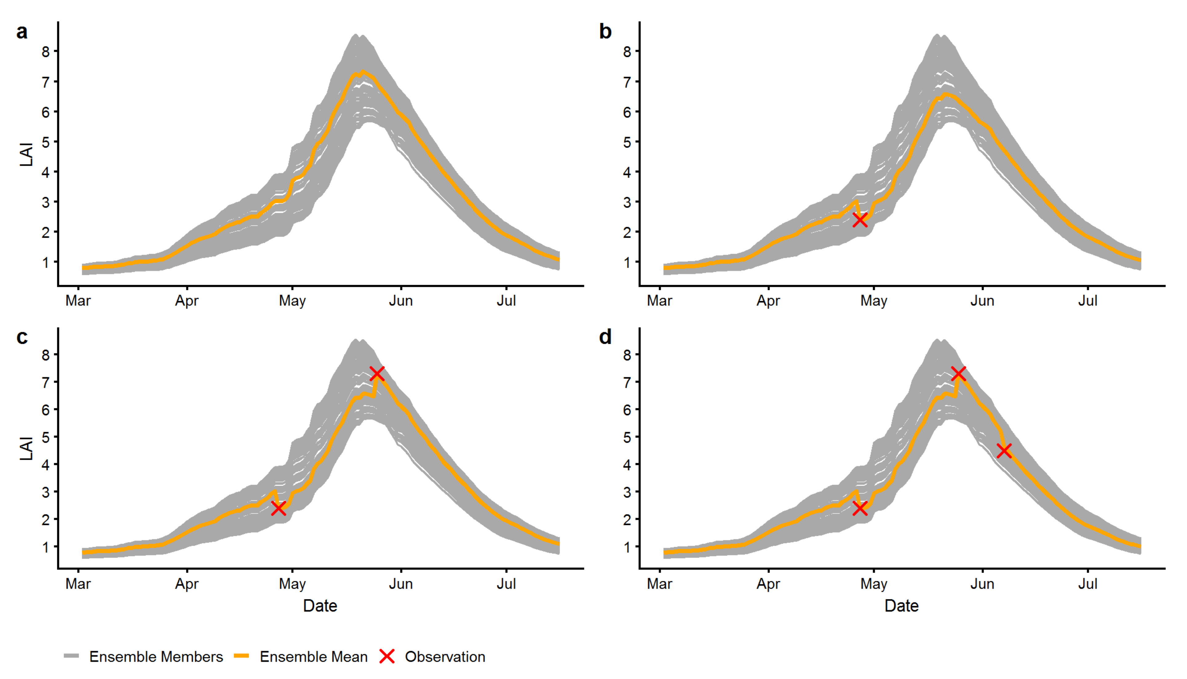
Example of Weighted Mean (WM) approach demonstrating the new ‘virtual data assimilation’ methodology. (a) An ensemble is created (orange line shows calculated mean of all ensemble members), (b) First LAI observation becomes available (red cross) and the contribution of each ensemble member to the ensemble mean is re-calculated, based on weights that depend on the proximity of the simulated value of the state variable to the observation (Equations (2) and (3)). The weights are propagated until (c) the next LAI observation becomes available, and a re-calculation of weights is triggered. (d) A third observation becomes available. No model ensemble member status variable is updated at any point in time.
Agronomy 10 00446 g001
Figure 2. 
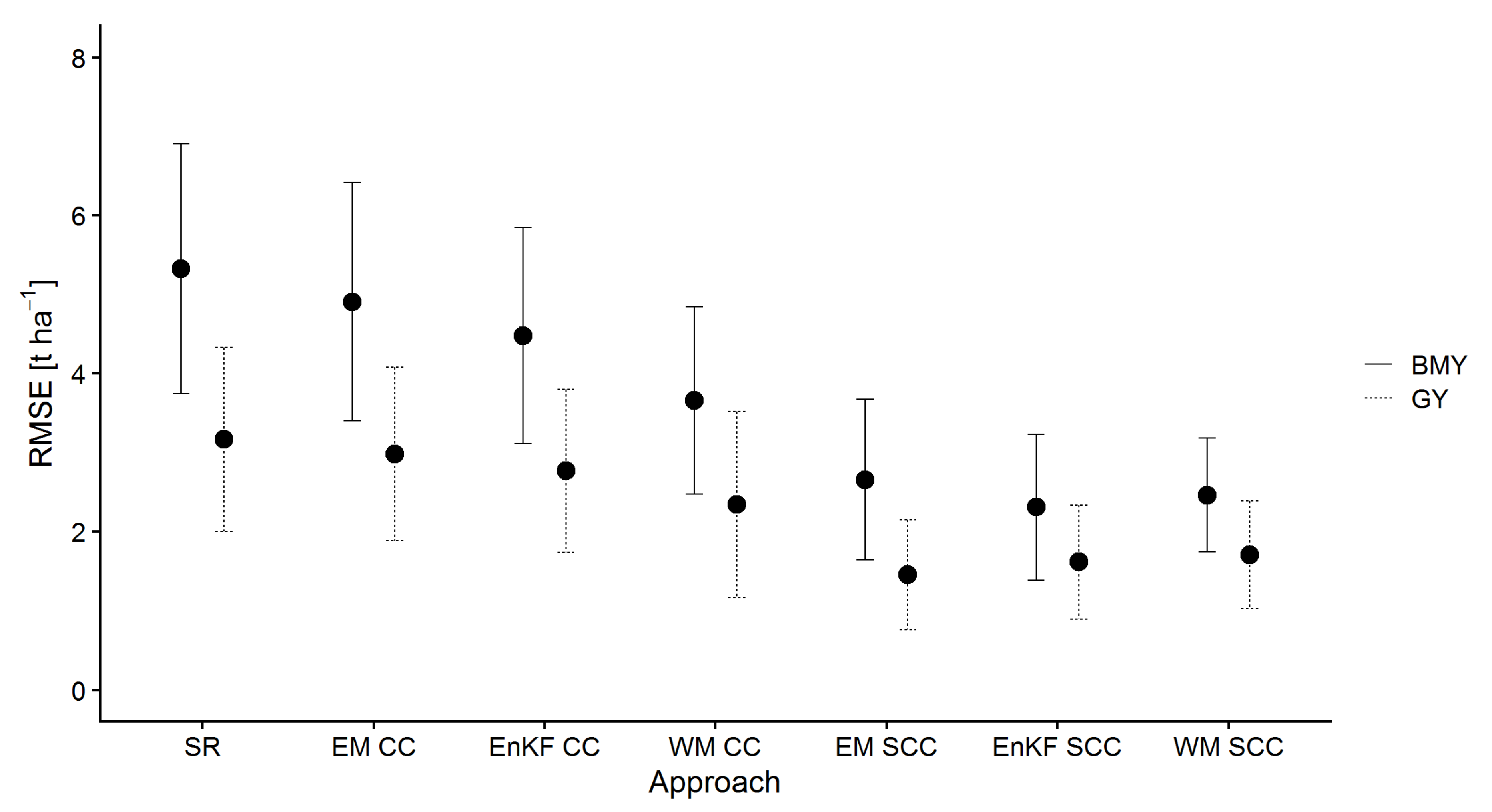
Mean and standard deviation of RMSE of total aboveground biomass yields (BMY—solid line) and grain yields (GY—dashed line) of 14 sites per approach. SR: Standard Run, EnKF: Ensemble Kalman Filter, WM: Weighted Mean, EM: Ensemble Mean, CC: Crop Component Set, SCC: Soil and Crop Component Set. All values in t ha−1.
Agronomy 10 00446 g002
Figure 3. 
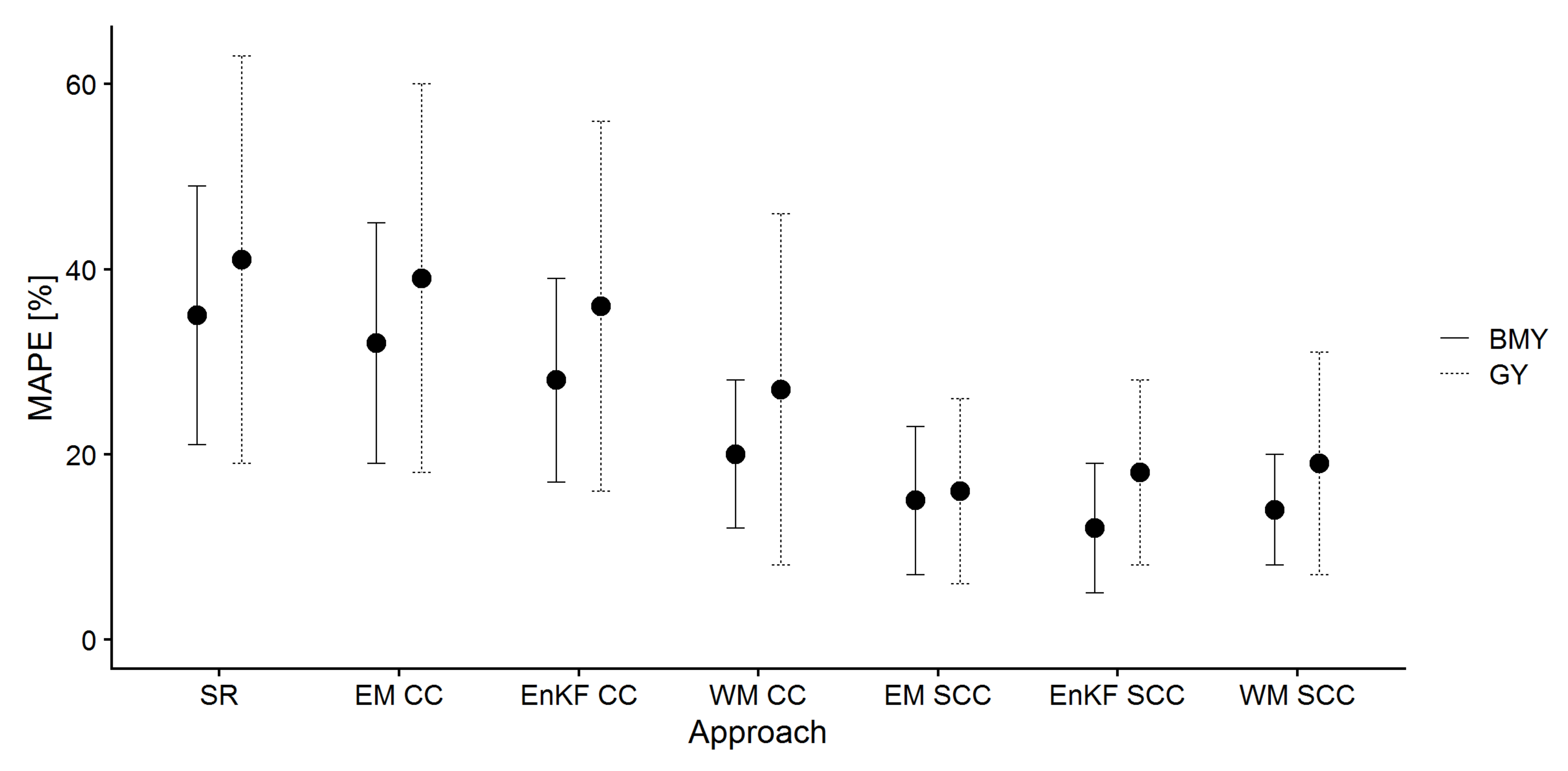
Mean and standard deviation of total aboveground biomass yields (BMY—solid line) and grain yields (GY—dashed line) mean absolute percentage error (MAPE in %) of 14 sites per approach. SR: Standard Run, EnKF: Ensemble Kalman Filter, WM: Weighted Mean, EM: Ensemble Mean, CC: Crop Component Set, SCC: Soil and Crop Component Set.
Agronomy 10 00446 g003
Figure 4. 
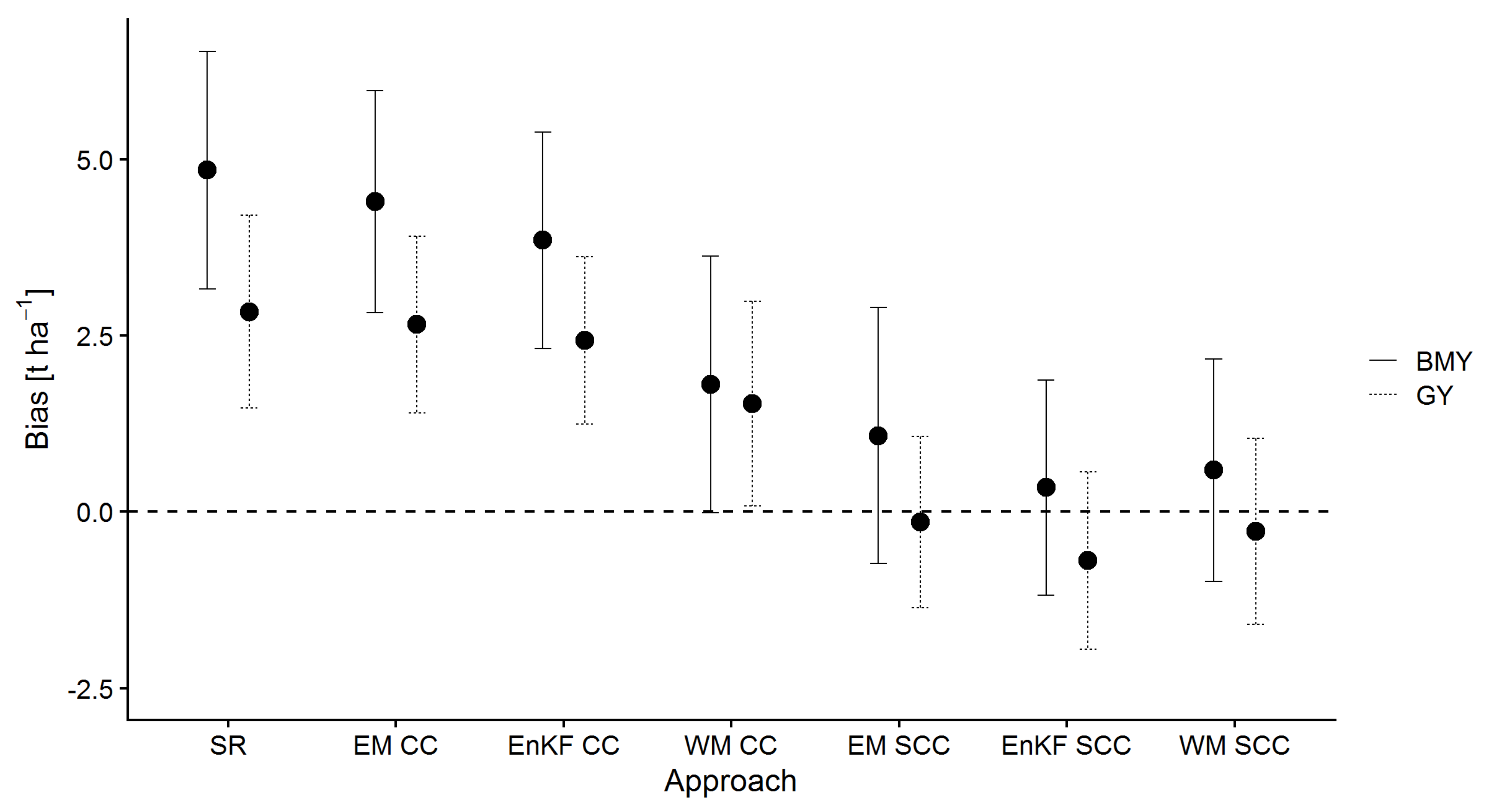
Mean and standard deviation of total aboveground biomass yield (BMY—solid line) and grain yield (GY—dashed line) bias of 14 sites per approach. SR: Standard Run, EnKF: Ensemble Kalman Filter, WM: Weighted Mean, EM: Ensemble Mean, CC: Crop Component Set, SCC: Soil and Crop Component Set. All values in t ha−1. Positive values indicate overestimation of the model, negative values indicate underestimation.
Agronomy 10 00446 g004
Table 1. List of study sites and locations. BMY: Average Total Aboveground Biomass Yield (t ha−1), GY: Average Grain Yield (t ha−1), HI: Harvest Index (HI = GY/BMY), DE: Germany, FR: France, NL: Netherlands.
CountryGrowing SeasonSiteLocationCultivar GrownPlanting DateBMYGYHI
DE2016/20171Central SaxonyBenchmark2016-10-1916.459.120.55
2016-11-30
DE2016/20172Southern Northrine-WestphaliaJonny2016-10-2514.555.970.41
DE2016/20173Northern HesseJulius2016-10-0419.5910.230.52
2016-10-28
DE2016/20174Northern BavariaRGT Reform2016-10-0517.379.050.54
2016-10-19
FR2016/20175Northwestern CharenteBologna2016-10-299.694.340.44
2016-11-15
FR2016/20176Northern OiseLyrik2016-10-0315.798.680.54
2016-10-18
NL2016/20177Eastern DrentheRGT Reform2016-10-1915.738.760.55
2016-11-03
2016-11-14
DE2017/20188Northern BavariaRGT Reform2017-11-0314.517.730.53
JB Asano
DE2017/20189RGT Reform2017-11-1616.408.090.49
JB Asano
DE2017/201810Central SaxonyRGT Reform2017-09-2118.8910.080.53
JB Asano
DE2017/201811RGT Reform2017-10-1618.829.540.50
JB Asano
DE2017/201812Central ThuringiaJB Asano2017-09-19, 2017-10-1912.425.270.42
RGT Reform
DE2017/201813Central Lower SaxonyRGT Reform2017-11-0314.518.080.55
JB Asano
DE2017/201814RGT Reform2017-10-1717.958.890.49
JB Asano
Table 2. Initial mean values for variables that were used by the Ensemble Kalman Filter (EnKF) to create a Gaussian distribution for ensemble generation, and range of values used by the Weighted Mean (WM) to create a uniform distribution for the ensemble generation. Two sets of variables were used: the crop component (CC) set or the combinational set of soil and crop components (SCC).
SetVariableEnKFWM
CCScaleFactorSLA10.75–1.25
ScaleFactorRUE10.75–1.25
RGRLAI0.008170.005–0.01134
SCCSoilWaterInit0.650.3–1
MaximalRootDepth1.250.5–2
ScaleFactorSLA1.250.75–1.25
Table 3. RMSE results for total aboveground biomass. SR: Standard Run, EnKF: Ensemble Kalman Filter, WM: Weighted Mean, EM: Ensemble Mean, CC: Crop Component Set, SCC: Soil and Crop Component Set. All values in t ha−1. DE: Germany, FR: France, NL: Netherlands.
CountrySiteSREM CCEnKF CCWM CCEM SCCEnKF SCCWM SCC
DE14.894.485.793.561.762.302.13
DE27.356.615.355.181.961.412.12
DE32.992.613.884.832.522.752.73
DE46.686.295.483.434.193.393.35
FR54.094.103.183.434.113.742.85
FR67.156.365.915.103.143.052.42
NL75.805.434.202.123.333.353.24
DE85.305.155.472.743.743.102.72
DE92.852.653.772.021.301.290.89
DE104.183.832.324.732.131.972.29
DE113.963.262.654.891.431.171.62
DE127.356.856.124.252.211.543.07
DE136.866.675.482.013.652.123.26
DE145.024.362.802.841.651.261.71
Mean5.324.904.463.652.652.322.46
SD1.581.501.341.181.010.900.71
Table 4. RMSE results for grain yields. SR: Standard Run, EnKF: Ensemble Kalman Filter, WM: Weighted Mean, EM: Ensemble Mean, CC: Crop Component Set, SCC: Soil and Crop Component Set. All values in t ha−1. DE: Germany, FR: France, NL: Netherlands.
CountrySiteSREM CCEnKF CCWM CCEM SCCEnKF SCCWM SCC
DE12.772.562.722.110.880.881.58
DE25.845.585.064.871.181.151.43
DE32.862.632.893.732.452.282.54
DE43.843.683.302.392.151.992.10
FR51.661.731.511.802.182.061.68
FR65.004.614.393.981.991.641.91
NL73.102.822.141.372.262.412.55
DE82.922.792.601.011.360.581.24
DE92.322.152.131.310.800.660.71
DE101.561.441.312.041.812.971.90
DE112.512.282.153.000.511.250.51
DE123.663.483.482.471.521.832.91
DE133.052.942.420.960.521.421.46
DE143.142.982.461.670.681.601.30
Mean3.162.982.752.341.451.621.70
SD1.161.091.031.170.690.690.68
Table 5. Mean absolute percentage (MAPE in %) results for total aboveground biomass. SR: Standard Run, EnKF: Ensemble Kalman Filter, WM: Weighted Mean, EM: Ensemble Mean, CC: Crop Component Set, SCC: Soil and Crop Component Set. DE: Germany, FR: France, NL: Netherlands.
CountrySiteSREM CCEnKF CCWM CCEM SCCEnKF SCCWM SCC
DE129263518101310
DE25146363212911
DE314121921121313
DE439363117221717
FR538393029333022
FR645403629131412
NL736332411161517
DE837363616251816
DE917162110774
DE102119112110810
DE1121171224657
DE1260564928151021
DE1348463710251221
DE1428241414868
Mean35322820151314
SD1413118866
Table 6. MAPE results for grain yields (in %, per site). EnKF: Ensemble Kalman Filter, WM: Weighted Mean, EM: Ensemble Mean, CC: Crop Component Set, SCC: Soil and Crop Component Set. DE: Germany, FR: France, NL: Netherlands.
CountrySiteSREM CCEnKF CCWM CCEM SCCEnKF SCCWM SCC
DE1302829218813
DE2100958680181720
DE327252732232124
DE442403524222121
FR532353237423933
FR659545143171316
NL734302110202225
DE83836331017615
DE929262614978
DE1014121117152615
DE11262422294124
DE1270666743243050
DE13383629951615
DE143533271551611
Mean41393527161819
SD2221201910912
Table 7. Bias results for total aboveground biomass per site. SR: Standard Run, EnKF: Ensemble Kalman Filter, WM: Weighted Mean, EM: Ensemble Mean, CC: Crop Component Set, SCC: Soil and Crop Component Set. All values in t ha−1. Positive values indicate overestimation of the model, negative values indicate underestimation. DE: Germany, FR: France, NL: Netherlands.
CountrySiteSREM CCEnKF CCWM CCEM SCCEnKF SCCWM SCC
DE14.574.125.581.960.751.76−0.40
DE27.266.515.154.441.610.870.96
DE32.562.093.513.402.022.262.16
DE45.905.424.680.872.972.142.46
FR52.112.291.621.38−2.54−2.16−0.95
FR66.055.174.713.98−0.970.24−0.33
NL74.884.403.01−1.02−1.91−2.28−2.71
DE85.054.874.82−0.373.382.132.04
DE92.772.543.36−0.071.100.00950.25
DE103.833.471.342.241.25−0.861.15
DE113.843.102.194.181.00−0.431.23
DE127.196.695.863.281.440.20−1.19
DE136.816.605.240.633.551.672.76
DE144.954.262.530.351.42−0.670.79
Mean4.844.393.831.801.070.340.58
SD1.681.571.511.821.811.531.57
Table 8. Bias results for grain yields per site. SR: Standard Run, EnKF: Ensemble Kalman Filter, WM: Weighted Mean, EM: Ensemble Mean, CC: Crop Component Set, SCC: Soil and Crop Component Set. All values in t ha−1. Positive values indicate overestimation of the model, negative values indicate underestimation. DE: Germany, FR: France, NL: Netherlands.
CountrySiteSREM CCEnKF CCWM CCEM SCCEnKF SCCWM SCC
DE12.652.412.581.33−0.120.16−0.76
DE25.775.514.974.630.950.910.57
DE32.692.442.673.132.231.992.29
DE43.192.992.620.980.35−0.060.55
FR5−0.090.240.610.19−1.75−1.62−1.25
FR64.494.073.883.35−1.24−0.41−0.96
NL72.572.221.36−0.25−1.78−2.03−2.24
DE82.912.772.520.331.330.161.09
DE92.292.122.100.940.72−0.460.57
DE101.090.940.500.43−1.39−2.74−1.34
DE112.482.242.052.76−0.11−1.190.03
DE123.553.363.392.16−1.10−1.64−2.49
DE133.002.882.260.31−0.02−1.250.23
DE143.082.902.341.12−0.11−1.41−0.19
Mean2.832.652.421.53−0.14−0.68−0.27
SD1.361.251.171.451.211.261.31

