Genetic and Environmental Predictors for Determining Optimal Seeding Rates of Diverse Wheat Cultivars


Abstract
1. Introduction
2. Materials and Methods
2.1. Site Description
2.2. Experimental Approach
2.3. Data Collection
2.4. Statistical Analyses and Modeling
3. Results
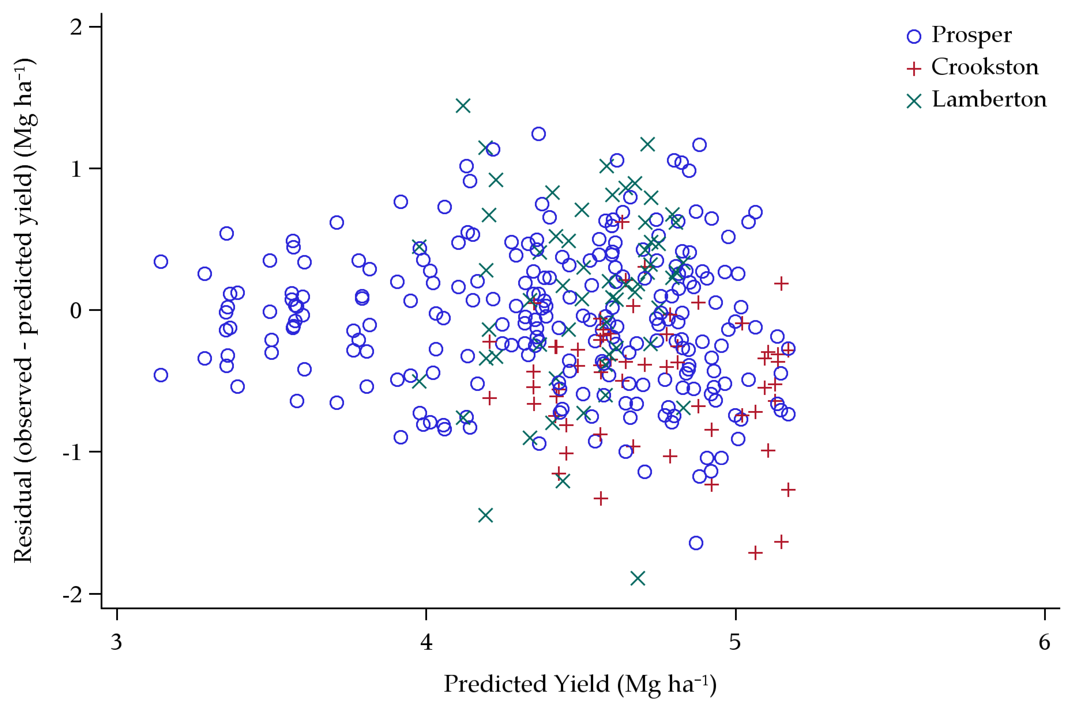
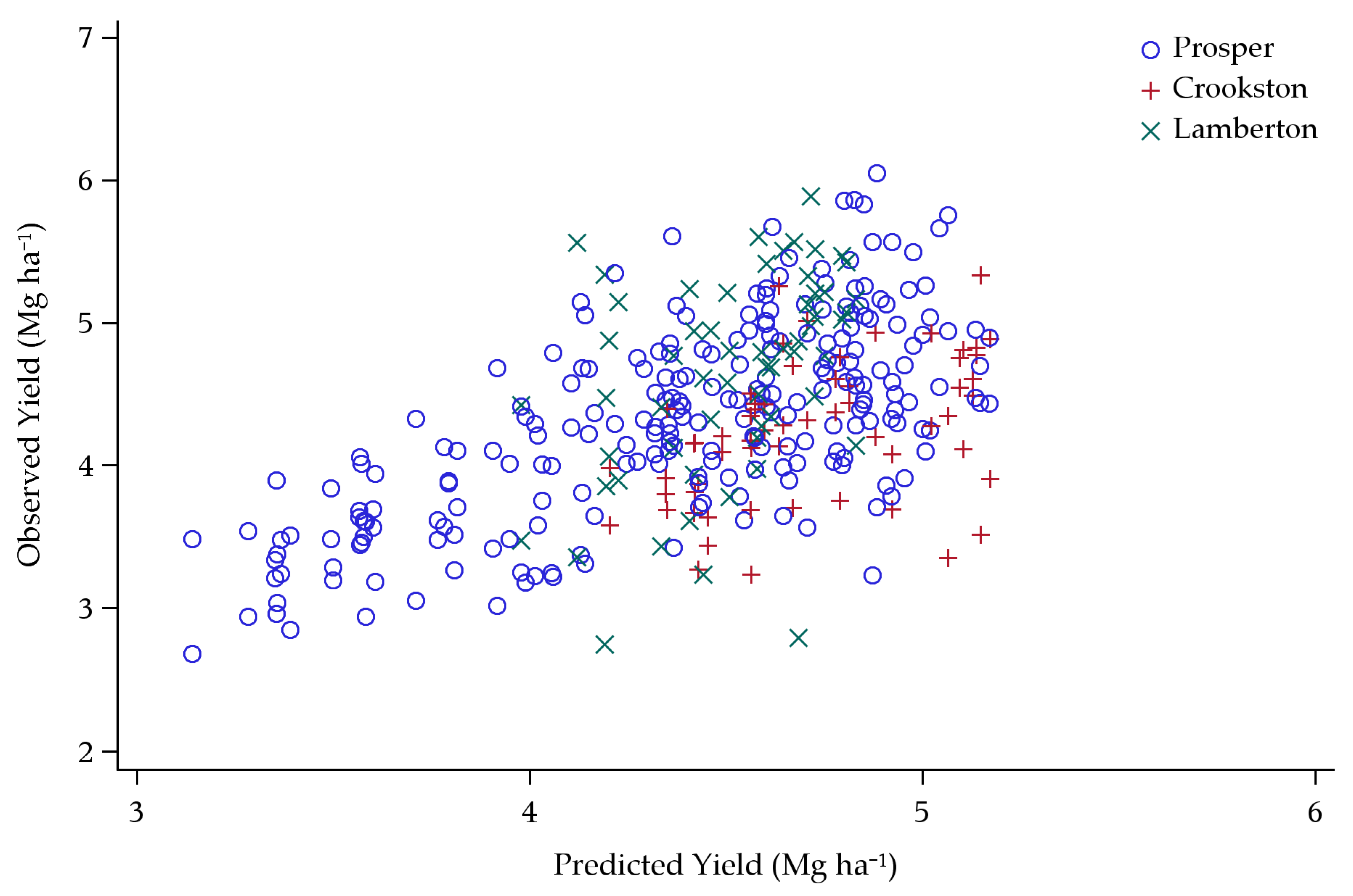
3.1. Original Yield Model
Model Predictions
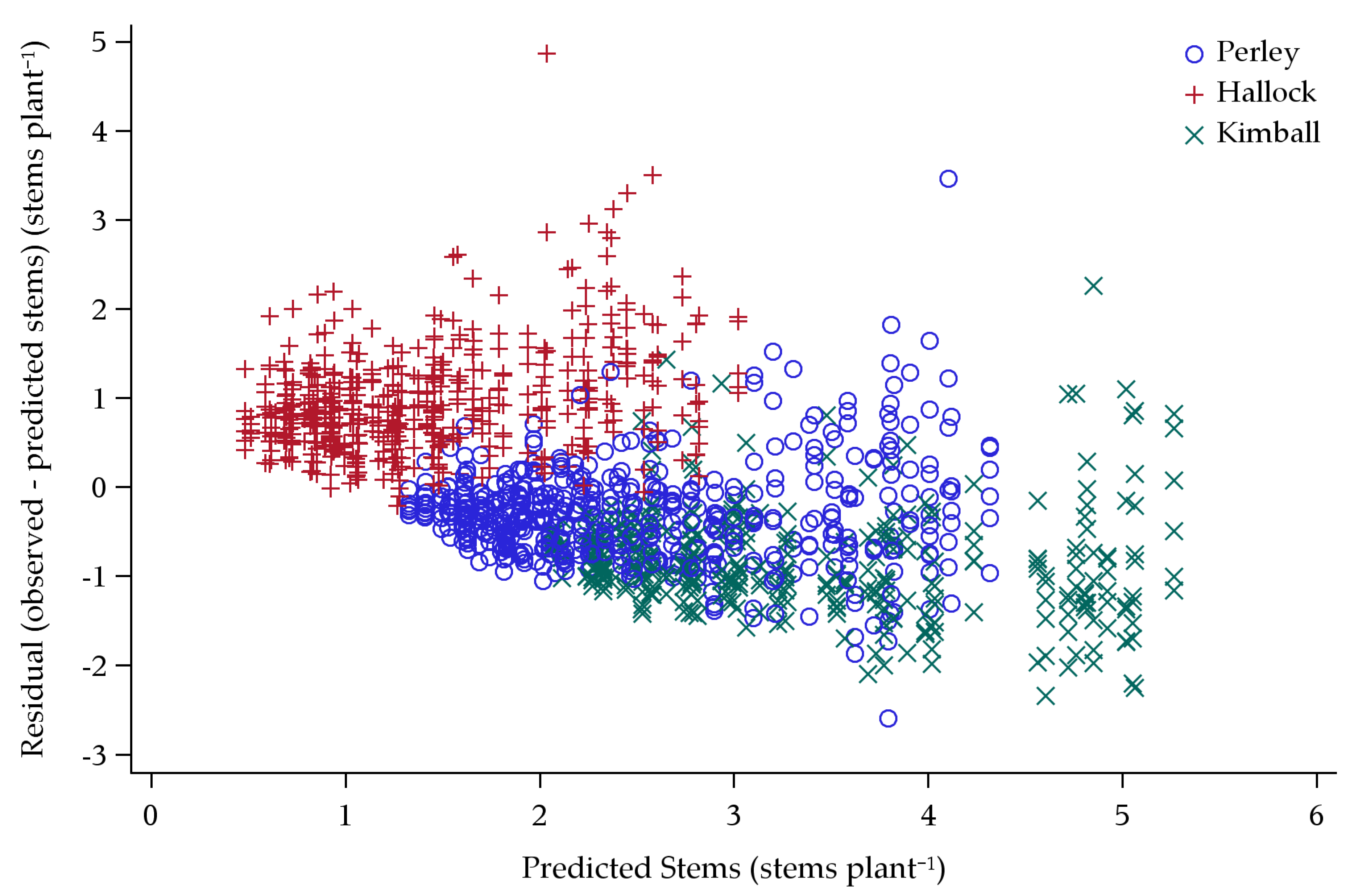
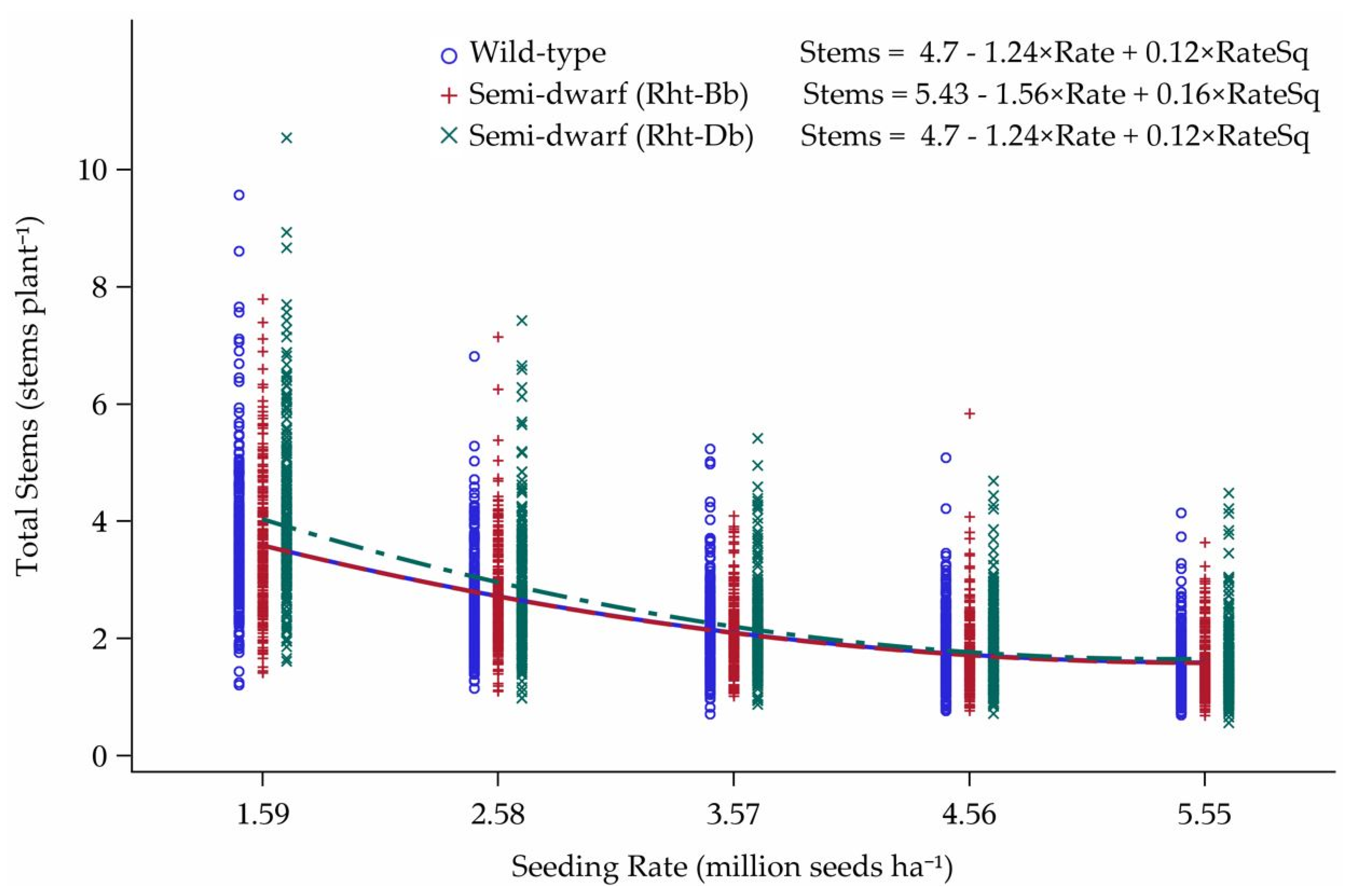
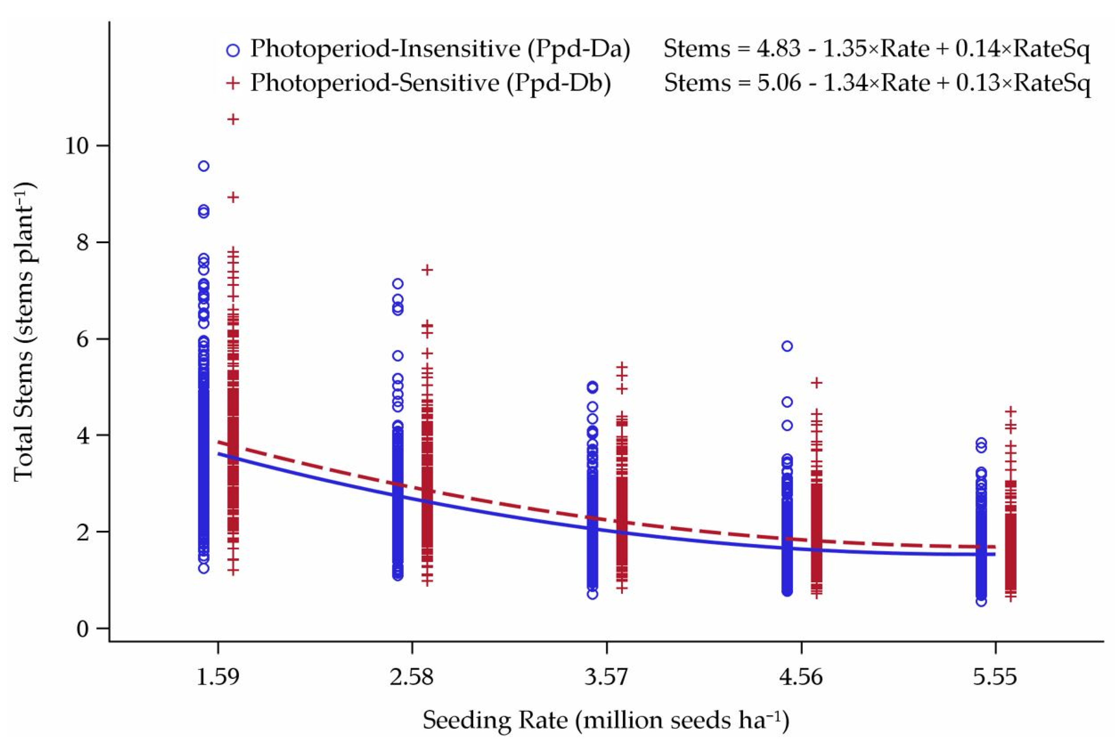
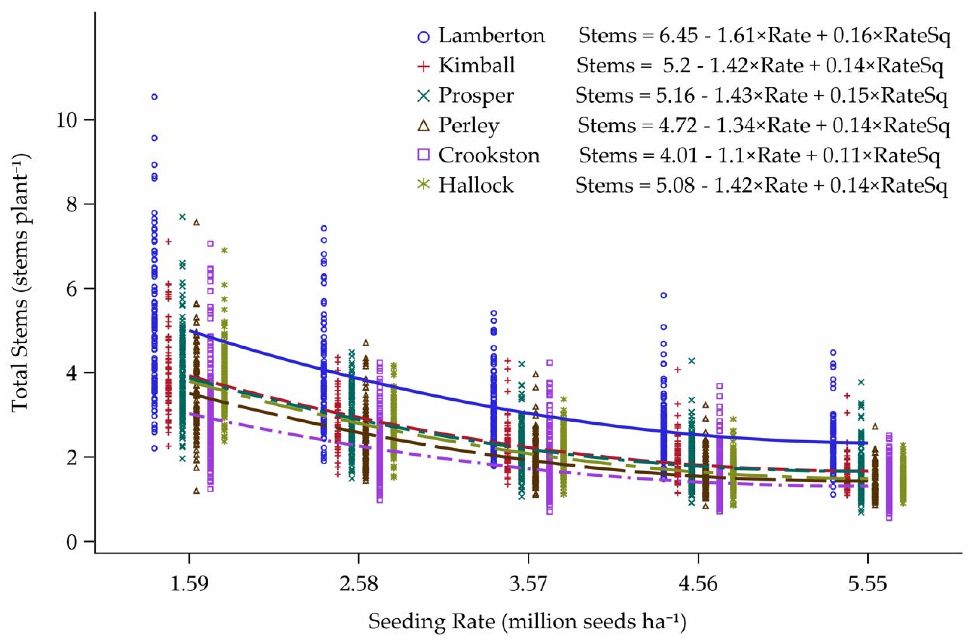
3.2. Tillering Model
Model Predictions
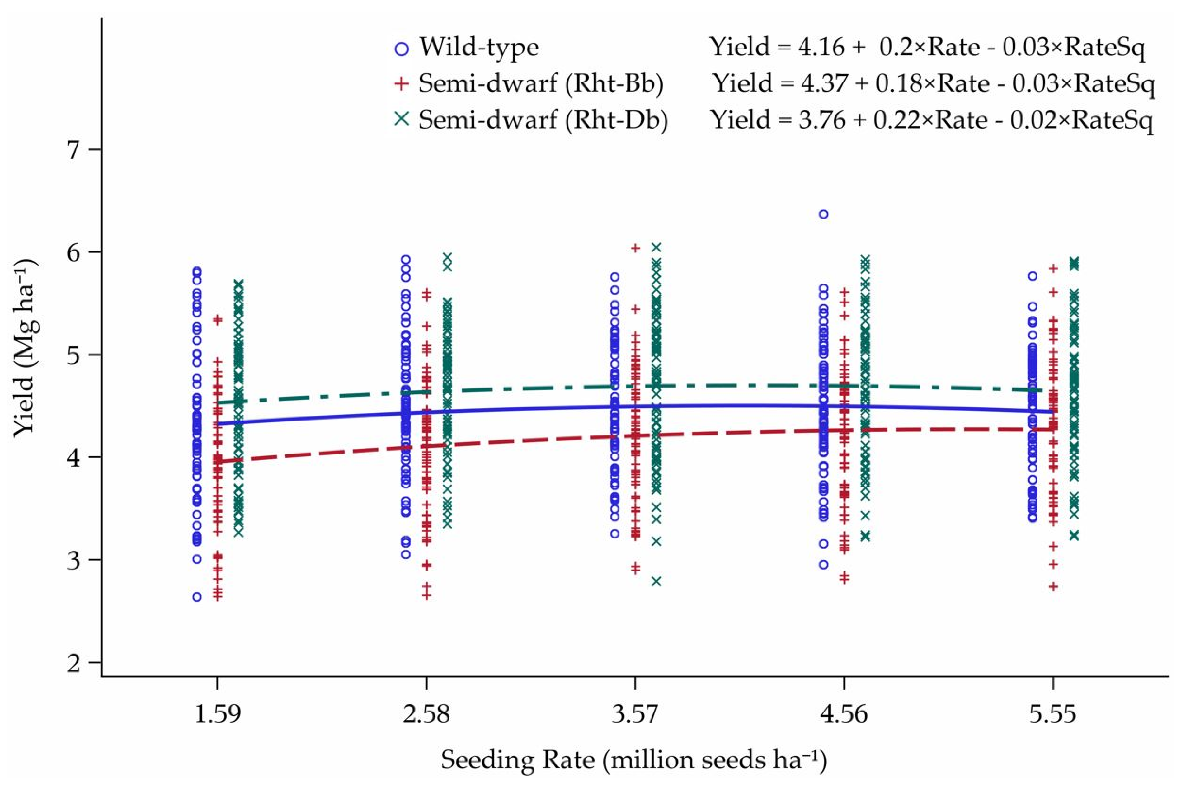
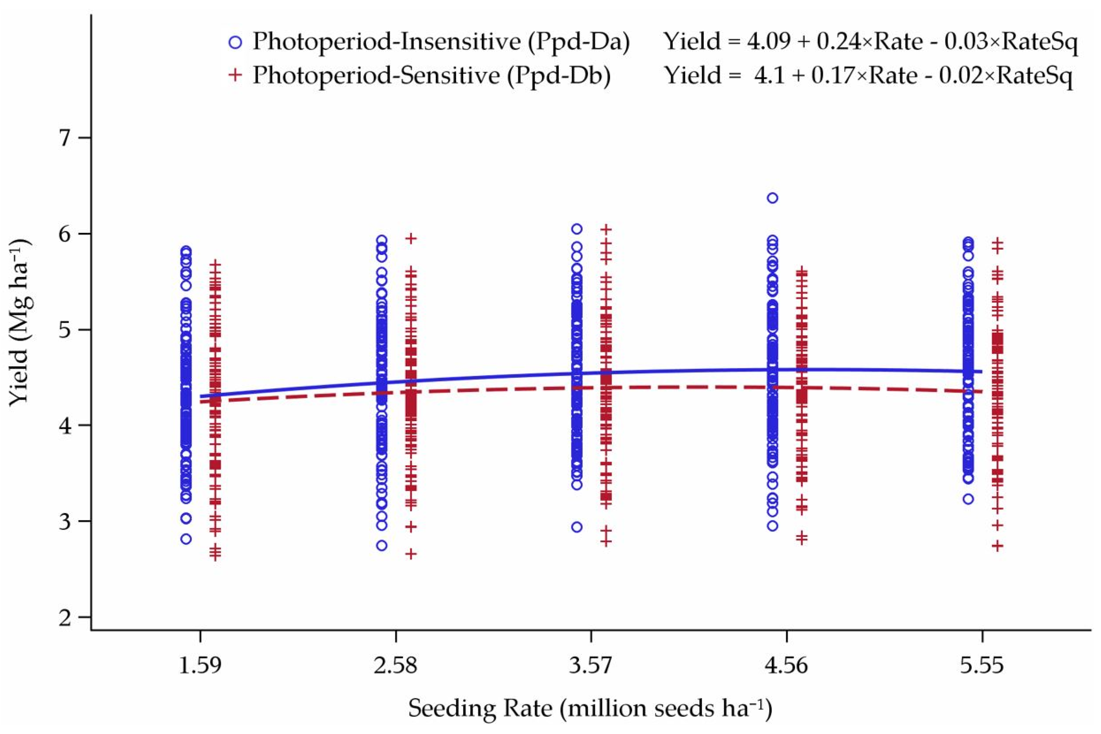
3.3. Reworked Yield Model
4. Discussion
4.1. Original Yield Model
4.2. Tillering Model
4.3. Yield Model Reworked
5. Conclusions
Author Contributions
Funding
Conflicts of Interest
References
- Baker, R.J. Effect of seeding rate on grain yield, straw yield, and harvest index of eight spring wheat cultivars. Can. J. Plant Sci. 1982, 62, 285–291. [Google Scholar] [CrossRef]
- Guitard, A.A.; Newman, J.A.; Hoyt, P.B. The influence of seeding rate on the yield and the yield components of wheat, oats, and barley. Can. J. Plant Sci. 1961, 41, 750–758. [Google Scholar] [CrossRef]
- Hanson, B.K.; Lukach, J.R. Barley response to planting rate in northeastern North Dakota. North Dakota Farm Res. North Dakota Agri. Exper. Station 1992, 14–19. [Google Scholar]
- Pendleton, J.W.; Dungan, G.H. The effect of seeding rate of nitrogen application on winter wheat cultivars with different characteristics. Agron. J. 1960, 52, 310–312. [Google Scholar] [CrossRef]
- Wiersma, J.J. Determining an optimum seeding rate for spring wheat in Northwest Minnesota. Crop. Manage. 2002, 18, 1–7. [Google Scholar] [CrossRef]
- Anderson, W.K.; Barclay, J. Evidence for differences between three wheat cultivars in yield response to plant population. Aust. J. Agric. 1991, 42, 701–713. [Google Scholar] [CrossRef]
- Briggs, K.G.; Aytenfisu, A. The effects of seeding rate, seeding date and location on grain yield, maturity, protein percentage and protein yield of some spring wheats in central Alberta. Can. J. Plant Sci. 1979, 59, 1139–1145. [Google Scholar] [CrossRef]
- Faris, D.G.; De Pauw, R.M. Effect of seeding rate on growth and yield of three spring wheat cultivars. Field Crops Res. 1981, 3, 289–301. [Google Scholar] [CrossRef]
- Kirby, E.J.M. The effect of plant density upon growth and yield of barley. Cambridge J. of Agr. Sci. 1967, 68, 317–324. [Google Scholar] [CrossRef]
- Butler, J.D.; Byrne, P.F.; Mohammadi, V.; Chapman, P.L.; Haley, S.D. Agronomic performance of Rht alleles in a spring wheat population across a range of moisture levels. Crop. Sci. 2005, 45, 939–947. [Google Scholar] [CrossRef]
- Lanning, S.P.; Martin, J.M.; Stougaard, R.N.; Guillen-Portal, F.R.; Blake, N.K.; Sherman, J.D. Evaluation of near-isogenic lines for three height-reducing genes in hard red spring wheat. Crop. Sci. 2012, 52, 1145–1152. [Google Scholar] [CrossRef]
- North Dakota State University Extension. North Dakota Hard Red Spring Wheat Variety Trial Results and Selection Guide; North Dakota State University Extension: Fargo, ND, USA, 2015; A574-15. [Google Scholar]
- Wiersma, J.J. A pilot project for determining the optimum seeding rates for individual HRSW cultivars. Minn. Wheat Res. Promot. Council Res. 2012.
- Hucl, P.; Baker, R.J. An evaluation of common spring wheat germplasm for tillering. Can. J. Plant Sci. 1988, 68, 1119–1123. [Google Scholar] [CrossRef]
- Worland, A.J. The influence of flowering time genes on environmental adaptability in European wheats. Euphytica 1996, 89, 49–57. [Google Scholar] [CrossRef]
- Friend, D.J.C. Tillering and leaf production in wheat as affected by temperature and light intensity. Can. J. Bot. 1965, 43, 1063–1076. [Google Scholar] [CrossRef]
- Li, W.L.; Nelson, J.C.; Chu, C.Y.; Shi, L.H.; Huang, S.H.; Liu, D.J. Chromosomal locations and genetic relationships of tiller and spike characters in wheat. Euphytica 2002, 125, 357–366. [Google Scholar] [CrossRef]
- Ciha, A.J. Seeding rate and seeding date effects on spring seeded small grain cultivars. Agron. J. 1983, 75, 795–799. [Google Scholar] [CrossRef]
- Baker, R.J. Agronomic performance of semi-dwarf and normal height spring wheats seeded at different dates. Can. J. Plant Sci. 1990, 70, 295–298. [Google Scholar] [CrossRef]
- Miralles, D.J.; Slafer, G.A. Yield, biomass and yield components in dwarf, semi-dwarf, and tall isogenic lines of spring wheat under recommended and late sowing dates. Plant Breed. 1995, 114, 392–396. [Google Scholar] [CrossRef]
- Borojevic, K. The transfer and history of ‘reduced height genes’ (Rht) in wheat from Japan to Europe. J. Heredity. 2005, 96, 455–459. [Google Scholar] [CrossRef]
- Gale, M.D.; Law, C.N.; Worland, A.J. Chromosomal location of a major dwarfing gene from Norin 10 in new British semi-dwarf wheats. Heredity 1975, 35, 417–421. [Google Scholar] [CrossRef]
- Gale, M.D.; Marshall, G.A. Chromosomal location of Gai-1 and Rht-1, genes for gibberellin insensitivity and semi-dwarfism, in a derivative of Norin-10 wheat. Heredity 1976, 37, 283–289. [Google Scholar] [CrossRef]
- Gale, M.D.; Law, C.N.; Marshall, G.A.; Snape, J.W.; Worland, A.J. Analysis and evaluation of semi-dwarfing genes in wheat including a major height reducing gene in variety “Sava”. IAEA-Tecdoc: Semi-dwarf Cereal Mutants Use Cross Breed. 1982, 268, 7–23. [Google Scholar]
- Scarth, R.; Law, C.N. The control of the day-length response in wheat by the group 2 chromosomes. Z Pflanzenzuchtg 1984, 92, 140–150. [Google Scholar]
- Davidson, J.L.; Christian, K.R. Flowering in wheat. In Control of Crop Productivity; Pearson, C.J., Ed.; Academic Press: Sydney, Australia, 1984; pp. 112–126. [Google Scholar]
- Busch, R.H.; Elsayed, F.A.; Heiner, R.E. Effect of daylength insensitivity on agronomic traits and grain protein in hard red spring wheat. Crop. Sci. 1984, 24, 1106–1109. [Google Scholar] [CrossRef]
- Dyck, J.A.; Matus-Cádiz, M.A.; Hucl, P.; Talbert, L.; Hunt, T.; Dubec, J.P. Agronomic performance of hard red spring wheat isolines sensitive and insensitive to photoperiod. Crop. Sci. 2004, 44, 1979–1981. [Google Scholar] [CrossRef]
- Marshall, L.; Nusch, R.; Cholick, F.; Edwards, I.; Frohberg, R. Agronomic performance of spring wheat isolines differing for daylength response. Crop. Sci. 1989, 29, 752–757. [Google Scholar] [CrossRef]
- Worland, A.J.; Appendino, M.L.; Sayers, E.J. The distribution in European winter wheats, of genes that influence ecoclimatic adaptability whilst determining photoperiodic insensitivity and plant height. Euphytica 1994, 80, 219–228. [Google Scholar] [CrossRef]
- Donald, C.M. Competition among crop and pasture plants. Adv. Agron. 1963, 15, 1–118. [Google Scholar]
- Holliday, R. Plant population and crop yield: Part I. Field Crop. Abstr. 1960, 13, 159–167. [Google Scholar]
- Hudson, H.G. Population studies with wheat: III. Seed rates in nursery and field plots. J. Agric. Sci. 1941, 31, 138–144. [Google Scholar] [CrossRef]
- Willey, R.W.; Heath, S.B. The quantitative relationships between plant population and crop yield. Adv. Agron. 1969, 21, 281–321. [Google Scholar]
- United States Department of Agriculture, Natural Resources Conservation Service. Web Soil Survey. Available online: http://websoilsurvey.nrcs.usda.gov/app/WebSoilSurvey.aspx (accessed on 13 January 2020).
- Fabrizius, E. Home Germination Testing of Wheat Seed; Kansas State Univ.: Manhattan, KS, USA; Kansas State Univ. Ext.: Manhattan, KS, USA, 2007; e-Update 98. [Google Scholar]
- Wiersma, J.J.; Ransom, J.K. The Small Grains Field Guide; North Dakota State Univ.: Fargo, ND, USA; North Dakota State Univ. Ext.: Manhattan, KS, USA, 2012; p. A-290. [Google Scholar]
- Large, E.C. Growth Stages in Cereals, Illustration of the Feekes Scale. Plant Pathol. 1954, 3, 128–129. [Google Scholar] [CrossRef]
- Ngo, T.H.D. The steps to follow in a multiple regression analysis. In Proceedings of the SAS Global Forum 2012 Conference, Orlando, FL, USA, 22–25 April 2012; SAS Institute Inc.: Cary, NC, USA, 2012. Paper 333. [Google Scholar]
- Sial, M.A.; Arain, M.A.; Javed, M.A.; Jamali, K.D. Genetic impact of dwarfing genes (Rht1 and Rht2) for improving grain yield in wheat. Asian J. Plant Sci. 2002, 1, 254–256. [Google Scholar]
- Pinthus, M.J.; Levy, A.A. The relationship between the Rht1 and Rht2 dwarfing genes and grain weight in Triticum aestivum L. spring wheat. Theor. Appl. Genet. 1983, 66, 153–157. [Google Scholar] [CrossRef] [PubMed]


| Location 1 | Year | Soil Series 2 | Soil Taxonomy 3 | Slope (%) |
|---|---|---|---|---|
| Lamberton, MN | 2014–15 | Webster | Fine-loamy, mixed, superactive, mesic Typic Endoaquolls | 0–2 |
| Normania | Fine-loamy, mixed, superactive, mesic Aquic Hapludolls | 0–2 | ||
| Kimball, MN | 2014 | Fairhaven | Fine–loamy over sandy or sandy-skeletal, mixed, superactive, mesic Typic Hapludolls | 0–2 |
| 2015 | Dakota | Fine-loamy over sandy or sandy-skeletal, mixed, superactive, mesic Typic Argiudolls | 2–6 | |
| Ridgeport | Coarse-loamy, mixed, superactive, mesic Typic Hapludolls | 2–6 | ||
| Prosper, ND | 2013–15 | Kindred-Bearden | Fine-silty, mixed, superactive, frigid Typic Endoaquolls | 0–2 |
| Perley, MN | 2013–15 | Fargo | Fine, smectitic, frigid Typic Epiaquerts | 0–1 |
| Crookston, MN | 2013, 2015 | Wheatville | Coarse-silty over clayey, mixed over smectitic, superactive, frigid Aeric Calciaquolls | 0–2 |
| Bearden-Colvin | Fine-silty, mixed, superactive, frigid Aeric Calciaquolls | 0–2 | ||
| 2014 | Wheatville | Coarse-silty over clayey, mixed over smectitic, superactive, frigid Aeric Calciaquolls | 0–2 | |
| Gunclub | Fine-silty, mixed, superactive, frigid Aeric Calciaquolls | 0–2 | ||
| Hallock, MN | 2013–15 | Northcote | Very-fine, smectitic, frigid Typic Epiaquerts | 0–1 |
| Photoperiodism | Plant Stature | |||
|---|---|---|---|---|
| Group | Cultivar | Ppd-D1 | Rht-B1 | Rht-D1 |
| 1 | Albany | b1 | b | a |
| Faller | b | b | a | |
| 2 | Knudson | a | b | a |
| Samson | a | b | a | |
| 3 | Briggs | b | a | a |
| Vantage | b | a | a | |
| 4 | Sabin | a | a | a |
| Oklee | a | a | a | |
| 5 | Kelby | a | a | b |
| Kuntz | a | a | b | |
| 6 | Marshall | b | a | b |
| Rollag | b | a | b | |
| Location | Planting Timing | Seeding Date | Harvest Date | Avg. Yield (Mg ha−1) |
|---|---|---|---|---|
| ―――――――――――――――― 2013 ―――――――――――――――― | ||||
| Crookston | Optimal | 10-May | 8-Aug | 6.14 |
| Crookston | Late | 29-May | 26-Aug | 6.38 |
| Hallock | Optimal | 16-May | 3-Sep | 7.27 |
| Perley | Optimal | 8-May | 16-Aug | 5.80 |
| Prosper | Optimal | 16-May | 22-Aug | 4.69 |
| ―――――――――――――――― 2014 ―――――――――――――――― | ||||
| Crookston | Optimal | 17-May | 27-Aug | 4.95 |
| Crookston | Late | 4-Jun | 27-Aug | 4.55 |
| Hallock | Optimal | 23-May | 6-Sep | 5.45 |
| Kimball | Optimal | 26-Apr | 14-Aug | 5.54 |
| Lamberton | Optimal | 21-Apr | 20-Aug | 5.14 |
| Perley | Optimal | 22-May | 2-Sep | 6.00 |
| Prosper | Optimal | 27-May | 3-Sep | 4.43 |
| ―――――――――――――――― 2015 ―――――――――――――――― | ||||
| Crookston | Optimal | 23-Apr | 21-Aug | 6.35 |
| Crookston | Late | 22-May | 25-Aug | 5.38 |
| Hallock | Optimal | 16-Apr | 13-Aug | 5.62 |
| Lamberton | Optimal | 4-Apr | 12-Aug | 5.62 |
| Lamberton | Late | 27-Apr | 12-Aug | 4.55 |
| Kimball | Optimal | 8-Apr | 31-Jul | 5.97 |
| Perley | Optimal | 13-Apr | 11-Aug | 7.03 |
| Prosper | Optimal | 9-Apr | 21-Aug | 4.67 |
| Prosper | Late | 22-May | 25-Aug | 3.62 |
| Gene Allele | Regression Equation 1 | Seeding Rate at Peak |
|---|---|---|
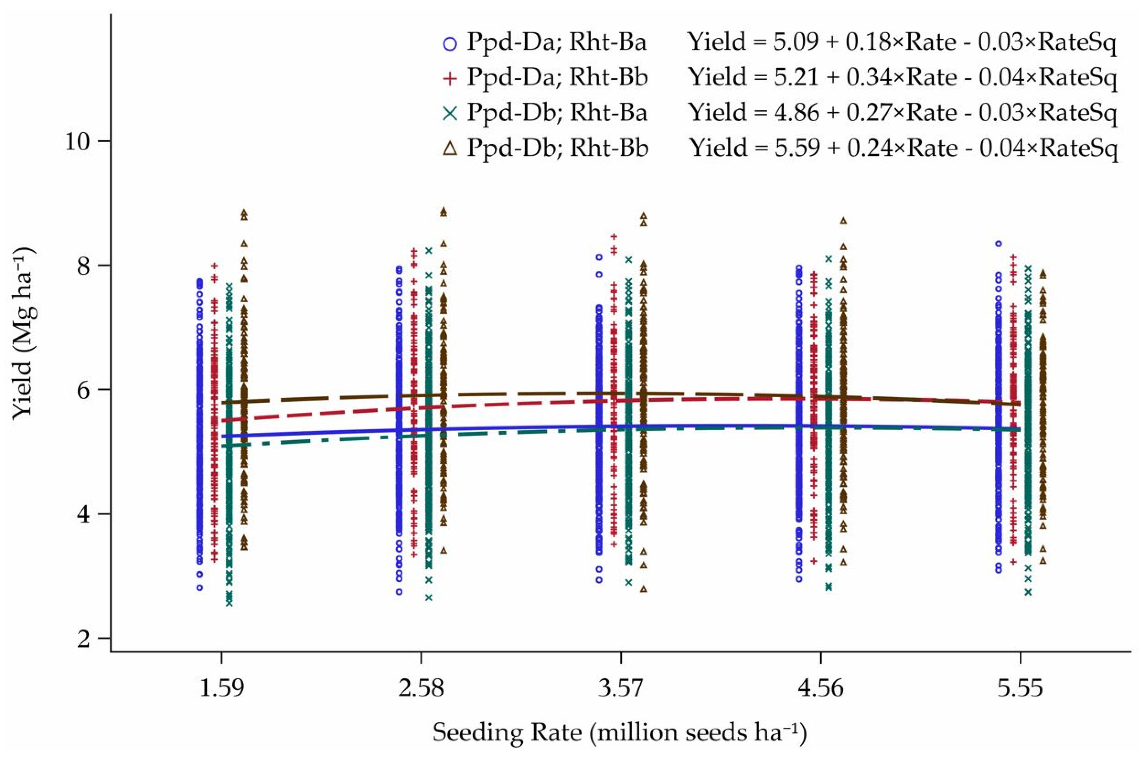
| Ppd-Da | Yield = 5.13 + 0.24×Rate – 0.03×RateSq | 3.69 million seeds ha−1 |
| Ppd-Db | Yield = 5.10 + 0.26×Rate – 0.04×RateSq | 3.59 million seeds ha−1 |
| Location | Regression Equation 1 | Seeding Rate at Peak |
|---|---|---|
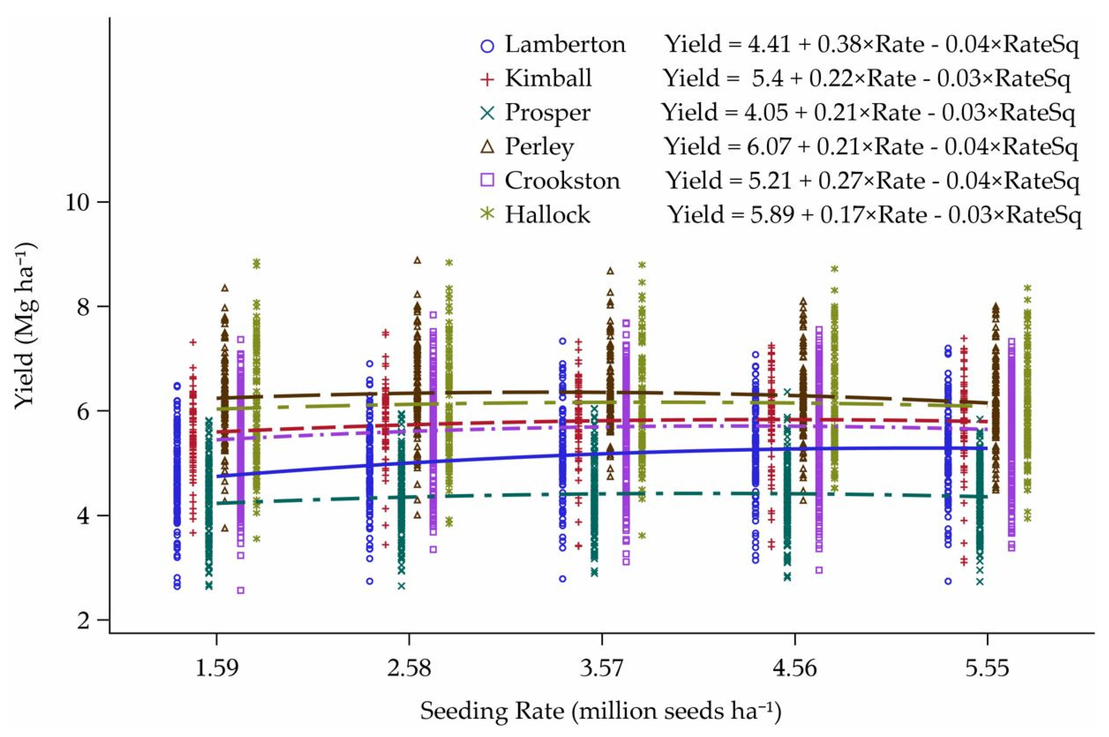
| Crookston | Yield = 5.40 + 0.29×Rate – 0.04×RateSq | 5.91 million seeds ha−1 |
| Lamberton | Yield = 4.09 + 0.24×Rate – 0.03×RateSq | 4.76 million seeds ha−1 |
| Prosper | Yield = 4.10 + 0.17×Rate – 0.02×RateSq | 3.53 million seeds ha−1 |
© 2020 by the authors. Licensee MDPI, Basel, Switzerland. This article is an open access article distributed under the terms and conditions of the Creative Commons Attribution (CC BY) license (http://creativecommons.org/licenses/by/4.0/).
Share and Cite
Mehring, G.H.; Wiersma, J.J.; Stanley, J.D.; Ransom, J.K. Genetic and Environmental Predictors for Determining Optimal Seeding Rates of Diverse Wheat Cultivars. Agronomy 2020, 10, 332. https://doi.org/10.3390/agronomy10030332
Mehring GH, Wiersma JJ, Stanley JD, Ransom JK. Genetic and Environmental Predictors for Determining Optimal Seeding Rates of Diverse Wheat Cultivars. Agronomy. 2020; 10(3):332. https://doi.org/10.3390/agronomy10030332
Chicago/Turabian StyleMehring, Grant H., Jochum J. Wiersma, Jordan D. Stanley, and Joel K. Ransom. 2020. "Genetic and Environmental Predictors for Determining Optimal Seeding Rates of Diverse Wheat Cultivars" Agronomy 10, no. 3: 332. https://doi.org/10.3390/agronomy10030332
APA StyleMehring, G. H., Wiersma, J. J., Stanley, J. D., & Ransom, J. K. (2020). Genetic and Environmental Predictors for Determining Optimal Seeding Rates of Diverse Wheat Cultivars. Agronomy, 10(3), 332. https://doi.org/10.3390/agronomy10030332