Abstract
The carbon footprint and energy cost of irrigation are increasing due to the modernization of irrigation systems, which also necessitates highly efficient use of water resources. Alternatives to conventional energy sources to power irrigation systems are renewable sources, primarily photovoltaic energy. Photovoltaic energy has the main disadvantage of producing a highly variable amount of energy, which affects the irrigation uniformity. Modeling irrigation systems in an integrated manner generates useful information about system performance for technicians that helps in the decision-making process. The EVASOR (EVAluation of SOlar iRrigation systems) model integrates different modules to simulate the whole solar irrigation system using a holistic approach: (1) I-Solar, which simulates the instantaneous power generated by the photovoltaic system, (2) AS-Solar, which simulates the variable speed pumping system, (3) Solar-Net, which simulates the hydraulic performance of the water distribution network, and (4) PRESUD-Irregular, which determines the discharge and pressure of all the emitters of the subunits together with irrigation quality parameters (coefficient of uniformity (CU), emission uniformity (EU), and coefficient of variation of the emitter discharge in the subunit (CVq) for any pressure at the subunit inlet. The integrated model EVASOR determines the irrigation quality parameters of complex irrigation systems with information on irradiance, air temperature, wind speed, and water table level for any combination of open subunits. To validate the model, results are presented regarding a case study located in southeast Spain.
1. Introduction
Two of the main challenges that humanity has to face are climate change and food security, which are linked. Agriculture plays a major role in facing these challenges. The demand for enough high-quality food for the world’s population has brought about changes in food production systems, wherein irrigation plays a key role. Irrigated agriculture produces 40% of food but represents only 18% of cultivated area [1], and has a significant impact on water resources. It represents 67% of the extraction of fresh water and 87% of the consumptive use of water [2]. Irrigated agriculture increased in area by 480% during the last century, and it is estimated that it will increase by another 30% by 2030 [3].
The lack of water resources is one of the main handicaps for agriculture in many areas in the world that face serious drought conditions. Besides the lack of water resources, the progressive increase in energy prices—about 3% per year since 2008 [4]—as well as the low price of harvests in the international market, are affecting the profitability of farms. The modernization of irrigation systems has led to an increase in energy efficiency, but also a linked increase in energy demand [5]. In pressurized networks, the energy consumed is a factor to be considered in terms of cost, which represents a high percentage of the total management, operation, and maintenance costs [6], as well as in terms of greenhouse gas emissions [7]. These aspects are especially important in areas where water is extracted from an aquifer, where extraction can account for up to 70% of the total energy demand on the irrigation scheme [8].
In this context, renewable energy—primarily solar energy—can supply long-term solutions, with very low greenhouse gas emissions [9]. Solar pumping systems offer several advantages [10] and are already being used in many regions of the world, such as the USA [11], India [12], Turkey [13], regions of Spain [5,14], and even in remote areas [15]. There are no data, at least not in Spain, that show the area irrigated with solar systems; however, the continuous increase in energy cost and the decrease in photovoltaic technology cost are driving factors behind the high interest of farmers in using this technology.
There is a need to develop management models that consider the highly variable energy production throughout the day, and the day of the year. Furthermore, the presence of clouds affects the continuity of energy production and, therefore, the irrigation uniformity.
Great effort has been made in the generation of photovoltaic simulation models [9,16,17,18,19,20], including energy generation forecasts [21]. Furthermore, there are many models for the hydraulic modeling of irrigation systems [5,22,23,24,25,26], large-scale water distribution networks [5,24,27,28,29] and pumping systems [6,30,31,32]. Several models that integrate water delivery systems with photovoltaic modeling have also been developed [9,33,34,35,36,37], as well as control algorithms for the integrated management of photovoltaic and hydraulic models [38]. However, there are no integrated models that permit the management—in an integrated manner—of complex irrigation systems energized with photovoltaic energy. Those models should accurately simulate the photovoltaic system, the irrigation system, the water distribution network, and the pumping system as an integrated scheme.
The main objective of an integrated solar pumping model is to determine the irrigation quality parameters, i.e., the coefficient of uniformity (CU), emission uniformity (EU), and coefficient of variation of the emitter discharge in the subunit (CVq), depending on the energy produced by the power generator in real time. Thus, a key issue is to simulate, in an accurate manner, the performance of the irrigation systems under different head pressures. To this end, [39] has developed the tool PRESUD-irregular, which performs hydraulic and energy analyses of drip and solid set irrigation systems for any shape of plot and topography, determining the discharge and pressure of all the emitters for any pressure at the subunit inlet. With these data, quality parameters of the irrigation events can be accurately determined. Advances linking the irrigation systems with the pumping system in integrated models have also been developed [26]. However, those models were based on an invariable energy supply. In the case of solar pumping systems, further developments must be made to accurately simulate the integrated systems, including the solar generator and its variable production. Furthermore, the performance of the pumping system is highly variable because it incorporates a variable frequency drive, in which the frequency is determined by the available power at the inlet of the system.
The objective of this work is the development and validation of an integrated solar pumping model, named EVASOR (EVAluation of SOlar iRrigation systems), to simulate complex irrigation systems with highly variable energy production. The model considers all the elements of the irrigation system, such as the photovoltaic generator, the pumping system, the water distribution networks, and the irrigation system in the plot. To validate the EVASOR model, intensive monitoring of the main electrical and hydraulic parameters was performed in a case study with a complex irrigation infrastructure.
2. Materials and Methods
In this work, a simulation model named EVASOR has been developed in MATLAB® (Mathworks Inc., Massachusetts, MA, USA). This model integrates the hydraulic and energy analysis of irrigation subunits, the hydraulic performance of the water distribution network, the performance of the pumping system, and the photovoltaic generator. Thus, it is an integrated simulation model used to perform the hydraulic and energy analysis of complex irrigation systems. These models are needed to perform high-quality irrigation in cases in which the energy production is highly variable, such as with solar pumping systems.
The EVASOR model is composed of four interconnected modules:
- I-Solar, the module of photovoltaic generators [40], which simulates the power generated in real time instead of the energy generated in a particular time interval.
- PRESUD-Irregular [39], the module to perform hydraulic analyses of irrigation systems in-plot.
- Solar-Net, the module to simulate water distribution networks, based on the EPANET engine, which implements a novel methodology to simulate the pressure and discharge at the head of the irrigation subunits.
- AS-Solar [41], which determines the performance of the variable speed pumping system. It also implements a novel methodology to perform a calibration process of the model using monitoring data.
2.1. I-Solar Module to Estimate the Solar Power Generated
The I-Solar module [40] permits accurate estimation of the generated photovoltaic power in real time from irradiance, temperature, and wind speed values. The Direct Insolation Simulation Code (DISC) [42], improved by [43], was implemented in this module for estimating the irradiance in inclined planes from irradiances in the horizontal plane. I-Solar integrates different algorithms to estimate AC power from irradiance on inclined planes. The main advantages it has over the existing models are:
- It determines the cell temperature using the air temperature, irradiance, and wind speed [44].
- It determines energy losses produced in the cables of the photovoltaic generator, the cable from the photovoltaic generator to the variable frequency drive, and from the variable frequency drive to the pump.
- The implementation of an algorithm of control that considers that the modules work on the point of maximum power, except when the generated power is higher than the demanded power, which makes the system move out of the point of maximum power. That is especially important when the photovoltaic generator is oversized, as in the “Peruelos” case study.
- It considers module aging using the linear method based on data supplied by the manufacturers.
- It characterizes in an accurate manner the performance of the variable frequency drive based on measured data, instead of data supplied by the manufacturer, which are usually too optimistic.
2.2. PRESUD-Irregular Module for Irrigation System Analysis
With the PRESUD-Irregular module [39], the hydraulic calculation of the irrigation subunit is performed. It allows for determining the discharge of every emitter for any pressure at the subunit inlet. With the value of discharge for all the emitters, it is possible to calculate the irrigation quality parameters. To perform the hydraulic analysis, the general emitter equation [45] is incorporated into the model, which can be supplied by the manufacturer or measured, as in this case study. PRESUD-Irregular uses the EPANET library [46] to perform the hydraulic calculation of the subunit, which has as many nodes as emitters. The elevation of each emitter is automatically obtained from the DEM generated with a drone, as described in the case study section. Head losses (hf) for PVC and LDPE are calculated using the Darcy–Weisbach equation (Equation (1)):
where hf is the pipe head loss (m), f is the friction factor, D is the internal pipe diameter (m), Q is the flow rate (m3 s−1), and L is the pipe length (m).
hf = 0.0826·f·D−5·Q2·L,
With this module, the following parameters can be estimated from any pressure at the subunit inlet: maximum, minimum, and average pressure; maximum, minimum, and average emitter discharge, total discharge in the subunit, and water velocity in pipes. With these data it is possible to determine irrigation quality parameters such as the coefficient of uniformity (CU, %), the total coefficient of variation of the emitter discharge in the subunit (CVq, %), and the emission uniformity (EU, %).
CU is calculated with Equation. (2) [47]:
where qi is the discharge of each emitter, qah is the mean of all emitter flow rate values due to variations in pressure (l h−1), and n is the number of emitters of the subunit.
CVq is calculated with Equation (3) [48]:
where Dq is the standard deviation of emitter discharge due to pressure variations and qah = average emitter discharge in the subunit due to pressure variation.
The emission uniformity (EU, %) [45] was modified by substituting the minimum discharge by the average discharge of the 25% of the drippers with lower discharge. This change was performed because, in subunits with a high variation in the elevation of drippers, EU is drastically decreased even when there are very few emitters with very low discharge.
where EU is the emission uniformity, e is the number of emitters per plant, CVqmf is the coefficient of variation of the emitters’ manufacturer, qm25% is the average of the 25% of the emitters with lower discharge values, and qah is the mean of all emitter discharge values due to variations in pressure (l h−1).
This irrigation quality parameter assumes normal distribution of the discharges in the subunit. This assumption is far from reality when the subunit is highly irregular in shape and is established in an irregular topography terrain. However, this irrigation quality parameter is widely used in the analysis of irrigation systems [25,49].
2.3. Module of Water Distribution Simulation, Solar-Net
To perform the hydraulic and energy analysis of the water distribution network, the Solar-Net module utilizes the EPANET library [46] and has been modified to allow hydraulic calculation with different discharge equations in the different nodes.
The general emitter equation [45] can be considered for each emitter in the different subunit of the irrigation system:
where qh = emission rate; K = emission coefficient; x = emission exponent; he = inlet pressure head of the emitter.
EPANET permits modifying the emission coefficient value, but it considers it to be the same for all the nodes. It allows for the inclusion of a different emission exponent for any node. The modification performed allows for introducing any emission coefficient for any node to EPANET, which makes it possible to simulate the network with different discharge equations in every node.
Once we have characterized all the subunits with the different nodes in EPANET, it would be possible to link all the subunits through the drawing of the irrigation network and simulate the complete hydraulic system. However, the inclusion of thousands of nodes makes the hydraulic calculation too computationally expensive and, in most cases, hydraulic convergence is not reached. To solve this problem, the discharge equations of the subunits are calculated by determining the total discharge of the subunit for different pressures at the subunit inlet. With the discharge equation of the subunit, the irrigation network is hydraulically analyzed thanks to the modification of EPANET described above.
Once the water distribution model has been characterized for any pressure at the head of the network and combination of open subunits, it is possible to determine the pressure at the origin of the open subunits and—with the results of PRESUD-Irregular—to determine the irrigation quality parameters in each subunit.
To calibrate the hydraulic model of the water distribution network, pressure values at strategic points of the networks were measured, and the roughness coefficient was calibrated, as described in [29].
2.4. Module of Pumping Systems Simulation, AS-Solar
AS-Solar [41] performs the hydraulic and energy simulation of pumping systems that abstract groundwater from wells. It incorporates the simulation of variable frequency drives, as in the case of solar pumping. To do so, the model implements the affinity laws (Equations (6) and (7)):
where Hvs is the pumping head at a variable speed (m); ηvs is the pump efficiency at a variable speed (%); and α is the ratio between the speed of the variable frequency drive and the maximum speed as a fixed frequency drive.
The main novelty of the model is the development of a calibration process that considers hydraulic, electrical, and pumping-related aspects. This process simulates the wear of the different elements of the pumping system. Impeller wear is simulated as an impeller cutting (Equations. (8) and (9)). A low value of λ means high wear on the impeller and a high value of λ means low wear.
where λ is the impeller diameter cut divided by the original impeller diameter (λ = Dr/Do).
Coefficient “C” of the Hazen–Williams equation (Equation (10)) is utilized to calibrate the hydraulics of the piping system [29,50]. A high value of C means low friction losses and a low value of C means high friction losses.
The electrical component is calibrated by including a term in the efficiency of the pumping system (ηelec) that considers the remaining components of the efficiency of the pumps (Equsation (11)). A low value of ηelec could mean an electrical problem.
With the proposed calibration procedure in the “Peruelos” case study, and the monitoring data described in Section 2.2, the impeller cutting resulted in λ = 0,9998, coefficient C = 65, and ηelec = 0.83. That means that the impellers are not worn out (λ value close to 1). The pumping pipe has a low value of C, compared with the theoretical value of 100 for steel, because the local losses are integrated in this coefficient [29] and because of possible decreases in the pipe diameter due to sedimentation [50]. The ηelec value integrates possible decreases in motor efficiency owing to the heating of the pump and other electrical losses.
With the calibrated model, accurate characteristic and efficiency curves can be obtained for any electrical frequency. Thus, depending on the electrical power available and considering the system curve obtained with Solar-Net, the working point is obtained using an iterative process that fits the power of the working point to the available power of the photovoltaic system.
Thus, with the EVASOR model we can determine the irrigation quality parameters, using the irradiance, temperature, and wind speed, for any combination of open subunits. This would permit the optimization of the management of the irrigation infrastructure powered with solar system.
2.5. The Case Study
To validate the EVASOR model, the irrigation infrastructure of the “Peruelos” farm was characterized. This farm is located in southeast Spain. The irrigated area is approximately 90 ha, and almond trees in a 7 × 7 m2 spacing are established. The irrigation system in the plot was subsurface drip irrigation. The area is divided into 20 irrigation subunits, with a highly irregular shape and topography (Table 1). Groundwater is extracted from a well approximately 215 m deep; the water level suffers extreme variations depending on the day of the year and the discharge of the system. The maximum discharge of the well is 7.5 L s−1.

Table 1.
Main characteristics of the subunits of the “Peruelos” case study.
A GNSS-RTK system Leica 1200 (Leica Geosystems AG, Heerbrugg, Switzerland) was utilized to measure the start and end of each irrigation lateral, valves, and other single elements. Thus, the irrigation system and the water distribution network were characterized. The estimated accuracy of global navigation satellite system-real time kinematic (GNSS-RTK) system is 0.02 m in planimetry and 0.03 m in altimetry. To characterize the topography of the whole area, a digital elevation model (DEM) was generated using a drone md4-200 (Microdrones, Inc., Kreuztal, Germany). By implementing the photogrammetry process [51], an accurate orthoimage and a DEM was obtained, with an accuracy in elevation of 0.07 m and a mesh of 0.05 m.
The pipe material of the water distribution network is PVC, with diameters ranging from 75 to 160 mm (Figure 1) of 0.6 MPa. In the case of the irrigation system in the plot, the material is PE for a diameter of 50 mm and PVC for a diameter of 63 mm, both of 0.6 MPa, and low-density polyethylene (LDPE) for a diameter of 32 mm. Lateral pipes are LDPE of 16 mm of 0.35 MPa.
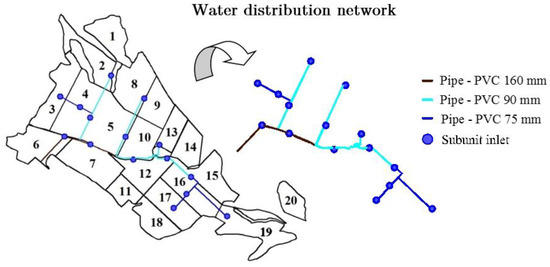
Figure 1.
Shape of the farm, localization of the sectors and scheme of the water distribution network.
The irrigation laterals integrate pressure-compensating drippers manufactured by John Deere (Deere and Company, Illinois, IL, USA), model HYDRO PCND, to a 1 m spacing. The pressure-compensating discharge of the drippers stated by the manufacturers is 1.75 l h−1. However, testing of the discharge curve (Figure 2) was performed following the standards ISO/FDIS 9261:2003(E) y ASAE STANDARDS 2004. A total of 24 drippers were evaluated at pressures from 50 to 300 kPa in steps of 50 kPa, the results of which are shown in Figure 2.
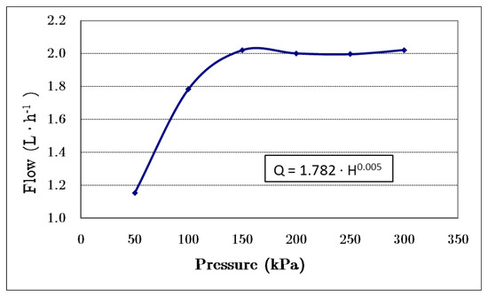
Figure 2.
Discharge curve of the dripper installed at the “Peruelos” farm.
The static water table level is around 130 m with a dynamic water table level during pumping of 190 m. A submersible pump DBM (DIBOMUR S.L., Murcia, Spain), model DX6-30 29-6 is installed 215 m deep, with a steel pumping pipe of 90 mm.
The photovoltaic generator is composed by 152 polycrystalline silicon modules (Table 2) Astronergy, model ASM6610P 265 (Astronergy/Chint Solar, Frankfurt, Germany), with eight lines and 19 modules per line. The total installed power is 40 kWp. The nominal power of the variable frequency drive is 30 kW. The generator is oriented south with a slope of 8.5°.
Table 2.
Characteristics of the photovoltaic module.
The variable frequency drive is 3G3RX-A4220-E1F (Omron Europe B.V., Hoofddorp, The Netherlands), with a nominal current of 57 and a maximum voltage of 800 V.
2.6. Monitoring System
The electrical, hydraulic, and energy parameters (Table 3) of the system were monitored every 10 min to calibrate and validate the model for the case study described above. Generated power in direct current (DC) was measured using an electrical network analyzer PEL 103 (Chauvin Arnoux, Paris, France). Transformed alternate current (AC) after the variable frequency drive was measured using an electrical network analyzer AR5 (CIRCUTOR, Barcelona, Spain). Both analyzers have an accuracy better than 1.5%. With this information, the efficiency of the variable frequency drive could be obtained for any generated power [32].
Table 3.
Main parameters for calibration and validation.
The main climatic parameters were horizontal plane irradiance (W m−2), measured with a Middleton EP07/134 calibrated pyranometer (Middleton Solar, Melbourne, Australia), and temperature (°C) and wind speed (m s−1), measured with an agroclimatic station SICO WS-600 (SICO Control Systems, Madrid, Spain).
The discharge of the pumping system was measured with a Woltman flowmeter WST-SB (Arad Group, Dalia, Israel), calibrated using a General Electric PT878 ultrasound flowmeter (General Electric Company, Boston, MA, USA). Pressure at the head of the irrigation network was measured using a WIKA pressure transducer, in the range 0–1 MPa (Instrumentos WIKA, S.A.U, Barcelona, Spain). The water table level was measured using a microtube and an air compressor.
The main parameters used for calibration and validation are shown in Table 3.
3. Results and Discussion
To showcase the applicability and validate the EVASOR model, it was applied to the “Peruelos” case study, utilizing the monitoring data described in the methodology. The results of the hydraulic analysis of the irrigation subunits and water distribution networks are presented and discussed, as well as the integration of the real-time solar power simulation and the performance of the pumping system. At the end of this section, the results of the integrated models are presented and discussed.
3.1. Hydraulic and Energy Analysis of Irrigation Subunits and Water Distribution Network
With PRESUD-Irregular, a hydraulic and energy analysis was performed for all the subunits, determining the discharge and pressure for all the emitters for any pressure at the subunit inlet. Thus, irrigation quality parameters were obtained. Owing to the high variability of the power generated by solar systems, a high variability in pressures at the subunit inlets appears during the irrigation events. With PRESUD-Irregular, a hydraulic and energy analysis for pressures at the subunit inlet from 1 m to the maximum working pressure of the pipes in the subunit was generated. As an example, Table 4 shows the results for subunits 1 and 10 of the case study. These two subunits are quite similar in area, but highly different in shape and topography (Table 1). In subunit 1, the maximum difference in elevation is equal to 19.3 m, while in subunit 10 it is 8.5 m. The hydrant of subunit 1 is located far from the subunit inlet, in the low elevation part of the subunit. The subunit 10 hydrant is located inside the subunit and in the high elevation part.
Table 4.
Hydraulic analysis results for subunits 1 and 10 under different pressures at the hydrant inlet.
A minimum value of EU = 85% was established to ensure the high quality of the irrigation event. Although these two subunits have a similar area, the differences found in shape and topography meant that in subunit 1, the minimum pressure to reach a EU = 85% was 344 kPa, with an average emitter discharge of 1.9 l h−1, while in the case of subunit 10, the minimum pressure was 37 kPa, with an average emitter discharge of 1.25 l h−1. For the same EU value, the average discharge can be different, which has a high impact on the irrigation time required to apply the required volume. Thus, the database generated with PRESUD-Irregular is useful in determining the proper management of the irrigation events, accounting for the time of irrigation and resultant quality. Furthermore, as shown in Figure 3, the discharge of all the emitters can be obtained for any pressure at the subunit inlet. This can help the managers of the irrigation systems to detect areas with systematic hydraulic problems and improve the system design so as to avoid them. Furthermore, the total volume of water applied to each area of the plot can be quantified if the pressure head is monitored at the subunit inlet.
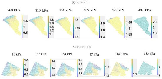
Figure 3.
Discharge distribution in subunit 1 and 10 for different values of pressure at the subunit inlet.
Table 5 shows the results of the hydraulic analysis of the 20 subunits that comprise the case study of the pressure at the subunit inlet that ensures an EU = 85%. Furthermore, it shows the pressure at the subunit inlet that ensures all the drippers are compensating (discharge 2 L h−1 and CVq = 0). The required pressure at the subunit inlet that ensures an EU = 85% is different for each subunit, from 37 kPa in subunit 10 to 346 kPa in subunit 18. These differences are due to differences in size, varying elevations of the drippers, and lateral lengths, among other factors. Without PRESUD-Irregular, it would be impossible to determine these pressure values and the irrigation quality parameters described in Table 5. There is a set of subunits with required pressure lower than 100 kPa (3, 5, and 10), and others with required pressure higher than 300 kPa (1, 6, 7, 11, and 18).
Table 5.
Results of the hydraulic performance and quality irrigation parameters for the different subunit of the case study for an EU = 85% and minimum compensating pressure.
The Solar-Net module objectivizes the analysis of the performance of the water distribution network and obtains the system curve for any combination of open subunits and any water lift in the well. The Solar-Net module requires the discharge equation of each subunit as an input (Figure 4), assuming that the whole subunit performs as one emitter. Using PRESUD-Irregular, the total discharge of the subunits can be obtained for any pressure at the subunit inlet, as in Table 4. Thus, the irrigation network is composed of 20 nodes, one for each subunit, and the linking pipes. For each node, a discharge equation is calculated with PRESUD-Irregular and introduced in Solar-Net. Then, using the modified EPANET software, which permits performing the hydraulic calculation considering nodes with different discharge equations, and given a set of open subunits, the pressure at the inlet of each open subunit can be obtained for any pressure at the head of the irrigation network. With the pressure at the subunit inlet and PRESUD-Irregular results, the irrigation quality parameters of the irrigation events can be determined. Figure 4 shows an example of the discharge equation for subunits 1 and 10, obtained with PRESUD-Irregular and introduced in Solar-Net to perform a hydraulic analysis of the water distribution network.
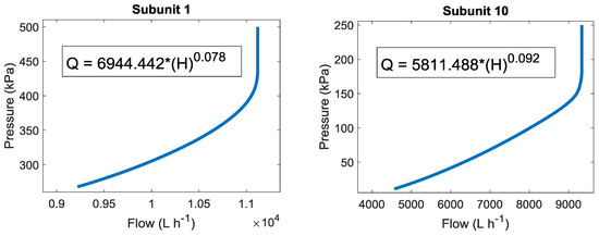
Figure 4.
Discharge equation of subunits 1 and 10.
The main purpose of the Solar-Net module is the generation of the system curve for any combination of open subunits and for any water table level. As an example, Figure 5 shows the system curves for different water table levels and when subunit 1 (a) and subunit 10 (b) are operating alone. Subunit 1 has a higher energy demand than subunit 10, because the subunit inlet elevations are 532.1 m and 519.5 m, respectively (Table 1). Furthermore, subunit 1 has a total discharge of 11,119 L h−1 (Table 4) at compensating pressure (437 kPa), while subunit 10 has 9336 L h−1 (at 183 kPa). Solar-Net is also able to determine the system curve for any combination of open subunits.
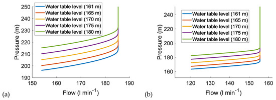
Figure 5.
System curves for different water table levels when subunit 1 (a) and subunit 10 (b) are open alone.
Once the system curve is obtained with the joint use of PRESUD-Irregular and Solar-Net, the working point for any rotation speed of the pump can be determined. It is determined as the crossing point of the characteristic curve, obtained with AS-Solar, and the system curve obtained with Solar-Net and PRESUD-Irregular. An iterative process is performed to fit the power supplied by the power generator, obtained with I-Solar, and the power required in the working point of pump and pipe system. To do so, the EVASOR model integrates all the modules and performs the energy and hydraulic analysis of the whole system.
3.2. Energy and Hydraulic Performance of the Whole System Using the EVASOR Model
To showcase the usefulness of the EVASOR model, it was applied for power values available at the pump inlet between 10 and 27 kW in steps of 1 kW in the case of: 1) subunit 3 in the open position and 2) subunits 3 and 11 in the open position. The hydraulic and energy characteristics of the subunits, pump efficiency and irrigation quality parameters are described in Table 6, Table 7 and Table 8. In the case that only subunit 3 is open, the system is not able to apply water up to 12 kW. Furthermore, to obtain an acceptable irrigation quality (EU = 85%), the power at the pump inlet should reach at least 14 kW. The increase in irrigation quality parameters in this subunit demands a high increase in the available power because of its large size and elevation (Table 1). Pressure compensation is given for a power of 21 kW. Increasing the power over 25 kW would exceed the working pressure limit of the pipe (588 kPa); at 26 kW, the subunit inlet pressure is 622 kPa. Thus, this subunit demands high power to irrigate with high quality, but care should be paid to not exceed the pipe’s working pressure, which results in a very low range of power for which this subunit could be activated alone without any problem. To avoid low quality parameters, this subunit should be activated when high power (high irradiance) is available; however, to avoid problems of limited pipe working pressure, at high power it should be opened jointly with another subunit. To evaluate this fact, Table 6 shows the performance of subunit 3 when it is activated jointly with subunit 11.
Table 6.
Hydraulic and energy conditions for different powers at pump inlet when subunit 3 is open.
Table 7.
Hydraulic and energy conditions of subunit 3 for different powers at pump inlet when subunits 3 and 11 are open.
Table 8.
Hydraulic and energy conditions of subunit 11 for different powers at pump inlet when subunits 3 and 11 are open.
The results regarding subunit 3 when open simultaneously with subunit 11 show that the minimum power for the pump inlet to irrigate is 16 kW (Table 7), as opposed to 12 kW when subunit 3 is activated alone (Table 6). Furthermore, to reach a minimum EU of 85%, the required power is 19 kW instead of 14 kW, and it is not possible to reach the compensating pressure and, therefore, the maximum discharge. However, when subunit 3 is activated together with subunit 11, there is no problem of limited pipe working pressure, because the maximum pressure at the subunit inlet is 213 kPa.
The results regarding the performance of subunit 11 when subunits 3 and 11 are open show that the pressure at the subunit inlet is higher than in the case of subunit 3, because the elevation of the subunit inlet is much lower (Table 1). The total discharge of subunit 11 suffered lower variations in power than subunit 3, because the subunit size is much smaller (2.2 ha for subunit 11, and 5.2 for subunit 3). Furthermore, because of the smaller size of subunit 11 compared to subunit 3, a decrease in CVq—when the generated power was increased to a higher rate—resulted in better quality parameters for medium-to-high power available at the pump inlet. The compensating pressure for subunit 11 was reached for a pump power of 25 kW, without any problem of pipe breaking. In no case was the maximum discharge of the well reached. If this were to happen, the model would reflect that.
Thus, EVASOR determined the power intervals for the proper performance of each subunit, and combinations of subunits open simultaneously. This permits technicians to determine the appropriate combination of open subunits depending on irradiance, temperature, and wind speed, together with the value of water lift in the well.
Further research and innovation actions needed for the implementation of this type of management tool are: (1) integrating the tool in automatic management tools to determine, in real time, the best combinations of subunits to irrigate depending on the above mentioned variables; (2) developing web-based tools to facilitate the access to the model to final users; (3) to implement the developed model in different sites all around the world, to showcase the usability of the model and to evaluate the water and energy savings obtained.
4. Conclusions
An innovative and intuitive model has been generated that accurately simulates the hydraulic and energy performance of complex irrigation systems energized with photovoltaic energy. It visualizes the pressure and discharge distribution in the irrigation subunit for any hydraulic condition, which permits detecting areas with irrigation problems and, therefore, helps with finding solutions.
EVASOR is an integrated model that analyzes the hydraulic and energy performance of the water distribution system as a whole, from the photovoltaic modules to the emitter. It is composed of four modules that—although able to work in an isolated manner—when integrated in EVASOR generate a powerful model able to accurately simulate the hydraulic and energy performance of complex irrigation systems.
The application to the “Peruelos” case study showcases the utility of this model, but also shows the necessity of the calibration of the different modules to perform accurate simulations of the system. Proper monitoring of the different components of the irrigation system is required to calibrate the simulation model, but the calibrated model also permits us to exploit the monitoring systems—going beyond the simple variable’s visualization functionality. The results obtained with EVASOR will permit us to determine the adequate irrigation quality parameters (knowing the amount and uniformity of irrigation water actually applied) for highly variable irrigation systems, determining the range of hours that each subunit or combination of subunits should be activated for. Furthermore, the results can be integrated into monitoring systems to perform semi-automatic subunit activations, depending on the historical data, the probability of the subunit being open, and the volume to apply.
Author Contributions
Conceptualization, J.C.-G., J.M.T. and M.A.M.; Data curation, J.C.-G., J.M., A.d.C. and M.A.M.; Formal analysis, J.C.-G., J.M. and M.A.M.; Funding acquisition, J.M.T. and M.A.M.; Investigation, J.C.-G., J.M. and M.A.M.; Methodology, J.C.-G., J.M. and M.A.M.; Project administration, M.A.M.; Resources, J.M., J.M.T. and M.A.M.; Software, J.C.-G., A.d.C. and M.A.M.; Supervision, J.M., J.M.T. and M.A.M.; Validation, J.C.-G. and J.M.; Visualization, J.C.-G., J.M. and M.A.M.; Writing—original draft, J.C.-G., J.M. and M.A.M.; Writing—review & editing, J.C.-G., J.M., J.M.T. and M.A.M. All authors have read and agreed to the published version of the manuscript.
Funding
This research was funded by the Spanish Ministry of Education and Science (MEC) NAME OF FUNDER, grant number AGL2017-82927-C3-2-R (Co-funded by FEDER) and the PRIMA program, supported under Horizon 2020 of the EU, grant number PRIMA-EU GA-1813.
Acknowledgments
We would like to thank Juan José Toboso, the owner of the Peruelos farm, for his unlimited help to us when carrying out this work. We would also like to thank the U.S. Sandia National Laboratories and the U.S. National Renewable Energy Laboratory (NREL) for their support and information, which made it possible to develop these models.
Conflicts of Interest
The authors declare no conflict of interest.
References
- Rockström, J.; Lannerstad, M.; Falkenmark, M. Assessing the water challenge of a new green revolution in developing countries. Proc. Natl. Acad. Sci. USA 2007, 104, 6253–6260. [Google Scholar] [CrossRef] [PubMed]
- Doll, P.; Siebert, S. Global modeling of irrigation water requirements. Water Resour. Res. 2002, 38, 1–10. [Google Scholar] [CrossRef]
- FAO; FIDA; PMA. El estado de la Inseguridad Alimentaria en el Mundo 2015; FAO: Rome, Italy, 2015; ISBN 9789253069279. [Google Scholar]
- European Commission. Energy Prices and Costs in Europe; European Commission: Brussels, Belgium, 2019. [Google Scholar]
- Tarjuelo, J.M.; Rodriguez-Diaz, J.A.; Abadía, R.; Camacho, E.; Rocamora, C.; Moreno, M.A. Efficient water and energy use in irrigation modernization: Lessons from Spanish case studies. Agric. Water Manag. 2015, 162, 67–77. [Google Scholar] [CrossRef]
- Moreno, M.A.; Ortega, J.F.; Córcoles, J.I.; Martínez, A.; Tarjuelo, J.M. Energy analysis of irrigation delivery systems: Monitoring and evaluation of proposed measures for improving energy efficiency. Irrig. Sci. 2010, 28. [Google Scholar] [CrossRef]
- Perry, C. Water footprints: Path to enlightenment, or false trail? Agric. Water Manag. 2014, 134, 119–125. [Google Scholar] [CrossRef]
- Córcoles, J.I.; de Juan, J.a.; Ortega, J.F.; Tarjuelo, J.M.; Moreno, M.a. Evaluation of Irrigation Systems by Using Benchmarking Techniques. J. Irrig. Drain. Eng. 2012, 138, 225–234. [Google Scholar] [CrossRef]
- Chandel, S.; Naik, M.; Energy, R.C.-R. Review of solar photovoltaic water pumping system technology for irrigation...: Heriot-Watt University Library Resources. Elsevier Renew. Sustain. Energy Rev. 2015, 49, 1084–1099. [Google Scholar] [CrossRef]
- Dursun, M.; Özden, S. Optimization of soil moisture sensor placement for a PV-powered drip irrigation system using a genetic algorithm and artificial neural network. Electr. Eng. 2017, 99, 407–419. [Google Scholar] [CrossRef]
- Vick, B.; Neal, B.; Clark, R.; Holman, A. Water Pumping with AC Motors and Thinfilm Solar Panels. In Proceedings of the Solar 2003 Conference; America’s Secure Energy: Austin, TX, USA, 2003; pp. 21–26. [Google Scholar]
- Pande, P.C.; Singh, A.K.; Ansari, S.; Vyas, S.K.; Dave, B.K. Design development and testing of a solar PV pump based drip system for orchards. Renew. Energy 2003, 28, 385–396. [Google Scholar] [CrossRef]
- Senol, R. An analysis of solar energy and irrigation systems in Turkey. Energy Policy 2012, 47, 478–486. [Google Scholar] [CrossRef]
- Reca, J.; Torrente, C.; López-Luque, R.; Martínez, J. Feasibility analysis of a standalone direct pumping photovoltaic system for irrigation in Mediterranean greenhouses. Renew. Energy 2016, 85. [Google Scholar] [CrossRef]
- Bouzidi, B. Viability of solar or wind for water pumping systems in the Algerian Sahara regions-Case study Adrar. Renew. Sustain. Energy Rev. 2011, 15, 4436–4442. [Google Scholar] [CrossRef]
- Aguilar, J.; Pérez-Higueras, P.; Almonacid, G. Average power of a photovoltaic grid-connected system. In Proceedings of the World Renewable Energy Congress IX, Florence, Italy, 19–25 August 2006. [Google Scholar]
- Jain, A.; Kapoor, A. A new method to determine the diode ideality factor of real solar cell using Lambert W-function. Sol. Energy Mater. Sol. Cells 2005, 85, 391–396. [Google Scholar] [CrossRef]
- Bellia, H.; Youcef, R.; Fatima, M. A detailed modeling of photovoltaic module using MATLAB. NRIAG J. Astron. Geophys. 2014, 3, 53–61. [Google Scholar] [CrossRef]
- Chouder, A.; Silvestre, S.; Sadaoui, N.; Rahmani, L. Modeling and simulation of a grid connected PV system based on the evaluation of main PV module parameters. Simul. Model. Pract. Theory 2012, 20, 46–58. [Google Scholar] [CrossRef]
- Ibrahim, I.A.; Khatib, T.; Mohamed, A.; Elmenreich, W. Modeling of the output current of a photovoltaic grid-connected system using random forests technique. Energy Explor. Exploit. 2018, 36, 132–148. [Google Scholar] [CrossRef]
- Antonanzas, J.; Osorio, N.; Escobar, R.; Urraca, R.; Martinez-de-Pison, F.J.; Antonanzas-Torres, F. Review of photovoltaic power forecasting. Sol. Energy 2016, 136, 78–111. [Google Scholar] [CrossRef]
- González Perea, R.; Camacho Poyato, E.; Montesinos, P.; Rodríguez Díaz, J.a. Critical points: interactions between on-farm irrigation systems and water distribution network. Irrig. Sci. 2014, 32, 255–265. [Google Scholar] [CrossRef]
- González Perea, R.; Camacho Poyato, E.; Montesinos, P.; Rodríguez Díaz, J.A. Prediction of irrigation event occurrence at farm level using optimal decision trees. Comput. Electron. Agric. 2019, 157, 173–180. [Google Scholar] [CrossRef]
- Díaz, J.A.R.; Poyato, E.C.; Pérez, M.B. Evaluation of water and energy use in pressurized irrigation networks in Southern Spain. J. Irrig. Drain. Eng. 2011, 137, 644–650. [Google Scholar] [CrossRef]
- Carrión, F.; Tarjuelo, J.M.; Carrión, P.; Moreno, M.a. Low-cost microirrigation system supplied by groundwater: An application to pepper and vineyard crops in Spain. Agric. Water Manag. 2013, 127, 107–118. [Google Scholar] [CrossRef]
- Carrión, F.; Sanchez-Vizcaino, J.; Corcoles, J.I.; Tarjuelo, J.M.; Moreno, M.A. Optimization of groundwater abstraction system and distribution pipe in pressurized irrigation systems for minimum cost. Irrig. Sci. 2016, 34, 145–159. [Google Scholar] [CrossRef]
- Fernández García, I.; González Perea, R.; Moreno, M.A.; Montesinos, P.; Camacho Poyato, E.; Rodríguez Díaz, J.A. Semi-arranged demand as an energy saving measure for pressurized irrigation networks. Agric. Water Manag. 2017, 193, 22–29. [Google Scholar] [CrossRef]
- González Perea, R.; Camacho, E.; Montesinos, P.; Rodríguez Díaz, J.A. Optimisation of water demand forecasting by artificial intelligence with short data sets. Biosyst. Eng. 2018, 1–8. [Google Scholar] [CrossRef]
- Moreno, M.A.; Planells, P.; Ortega, J.F.; Tarjuelo, J.M. Calibration of On-Demand Irrigation Network Models. J. Irrig. Drain. Eng. 2008, 134, 36–42. [Google Scholar]
- Izquiel, A.; Ballesteros, R.; Tarjuelo, J.M.; Moreno, M.A. Optimal reservoir sizing in on-demand irrigation networks: Application to a collective drip irrigation network in Spain. Biosyst. Eng. 2016, 147. [Google Scholar] [CrossRef]
- Jackson, T.M.; Khan, S.; Hafeez, M. A comparative analysis of water application and energy consumption at the irrigated field level. Agric. Water Manag. 2010, 97, 1477–1485. [Google Scholar] [CrossRef]
- Moreno, M.A.; Carrión, P.A.; Planells, P.; Ortega, J.F.; Tarjuelo, J.M. Measurement and improvement of the energy efficiency at pumping stations. Biosyst. Eng. 2007, 98, 479–486. [Google Scholar] [CrossRef]
- Zerhouni, F.Z.; Zerhouni, M.H.; Zegrar, M.; Benmessaoud, M.T.; Stambouli, A.B.; Midoun, A. Proposed methods to increase the output efficiency of a photovoltaic (PV) system. Acta Polytech. Hungarica 2010, 7, 55–70. [Google Scholar]
- Shen, C.; He, Y.L.; Liu, Y.W.; Tao, W.Q. Modelling and simulation of solar radiation data processing with Simulink. Simul. Model. Pract. Theory 2008. [Google Scholar] [CrossRef]
- Poompavai, T.; Kowsalya, M. Control and energy management strategies applied for solar photovoltaic and wind energy fed water pumping system: A review. Renew. Sustain. Energy Rev. 2019, 108–122. [Google Scholar] [CrossRef]
- Li, G.; Jin, Y.; Akram, M.W.; Chen, X. Research and current status of the solar photovoltaic water pumping system—A review. Renew. Sustain. Energy Rev. 2017, 79, 440–458. [Google Scholar] [CrossRef]
- Aliyu, M.; Hassan, G.; Said, S.A.; Siddiqui, M.U.; Alawami, A.T.; Elamin, I.M. A review of solar-powered water pumping systems. Renew. Sustain. Energy Rev. 2018, 87, 61–76. [Google Scholar] [CrossRef]
- González Perea, R.; Mérida García, A.; Fernández García, I.; Camacho Poyato, E.; Montesinos, P.; Rodríguez Díaz, J.A. Middleware to Operate Smart Photovoltaic Irrigation Systems in Real Time. Water 2019, 11, 1508. [Google Scholar] [CrossRef]
- Moreno, M.A.; del Castillo, A.; Montero, J.; Tarjuelo, J.M.; Ballesteros, R. Optimisation of the design of pressurised irrigation systems for irregular shaped plots. Biosyst. Eng. 2016, 151. [Google Scholar] [CrossRef]
- Cervera, J.; Del Castillo, A.; Montero, J.; Laserna, S.; Tarjuelo, J.M.; Moreno, M.A. Modelo de cálculo de la irradiancia solar semi-horaria sobre superficie inclinada para instalaciones fotovoltaicas. In Proceedings of the 20th International Congress on Project Management and Engineering, Cartagena, Colombia, 13–15 July 2016. [Google Scholar]
- Cervera, J.; del Castillo, A.; Montero, J.; Tarjuelo, J.M.; Moreno, M.Á. Calculation model for solar-powered drip irrigation management. In Proceedings of the 22th International Congress on Project Management and Engineering, Madrid, Spain, 11–13 July 2018. [Google Scholar]
- Maxwell, E.L. A quasi-physical model for converting hourly Global Horizontal to Direct Normal Insolation. Sol. Energy Res. Inst. 1987. [Google Scholar]
- Perez, R.R.; Ineichen, P.; Maxwell, E.L.; Seals, R.D.; Zelenka, A. Dynamic Global-to-Direct Irradiance Conversion Models; Ashrae Transactions: Baltimore, MD, USA, 1992. [Google Scholar]
- King, D.L.; Kratochvil, J.a.; Boyson, W.E. Photovoltaic array performance model. Online 2004. [Google Scholar] [CrossRef]
- Keller, J.; Bliesner, R.D. Sprinkle and Trickle Irrigation; Van Nostrand Reinhold: New York, NY, USA, 1990. [Google Scholar]
- Rossman, L. a EPANET 2: users manual. Cincinnati US Environ. Prot. Agency Natl. Risk Manag. Res. Lab. 2000, 38, 200. [Google Scholar] [CrossRef]
- Christiansen, J.E. Irrigation by Sprinkling; ISBN University of California Agricultural Experiment Station Bulletin 670; University of California: Auckland, CA, USA, 1942. [Google Scholar]
- Bralts, V.F.; Edwards, D.M.; Wu, L.-P. Drip irrigation design and evaluation based on the statistical uniformity concept. Adv. Irrig. 1987, 4, 67–117. [Google Scholar]
- Carrión, F.; Tarjuelo, J.M.; Hernández, D.; Moreno, M.a. Design of microirrigation subunit of minimum cost with proper operation. Irrig. Sci. 2013, 31, 1199–1211. [Google Scholar] [CrossRef]
- Abadía, R. Optimización del Diseño y gestión de Redes Colectivas de Distribución de Agua para Riego por Goteo de Cultivos Leñosos; Aplicación al regadío de Mula (Murcia), Universidad Miguel Hernández: Elche, Spain, 2003. [Google Scholar]
- Ballesteros, R.; Ortega, J.F.; Hernández, D.; Moreno, M.A. Applications of georeferenced high-resolution images obtained with unmanned aerial vehicles. Part I: Description of image acquisition and processing. Precis. Agric. 2014, 15. [Google Scholar] [CrossRef]


© 2020 by the authors. Licensee MDPI, Basel, Switzerland. This article is an open access article distributed under the terms and conditions of the Creative Commons Attribution (CC BY) license (http://creativecommons.org/licenses/by/4.0/).