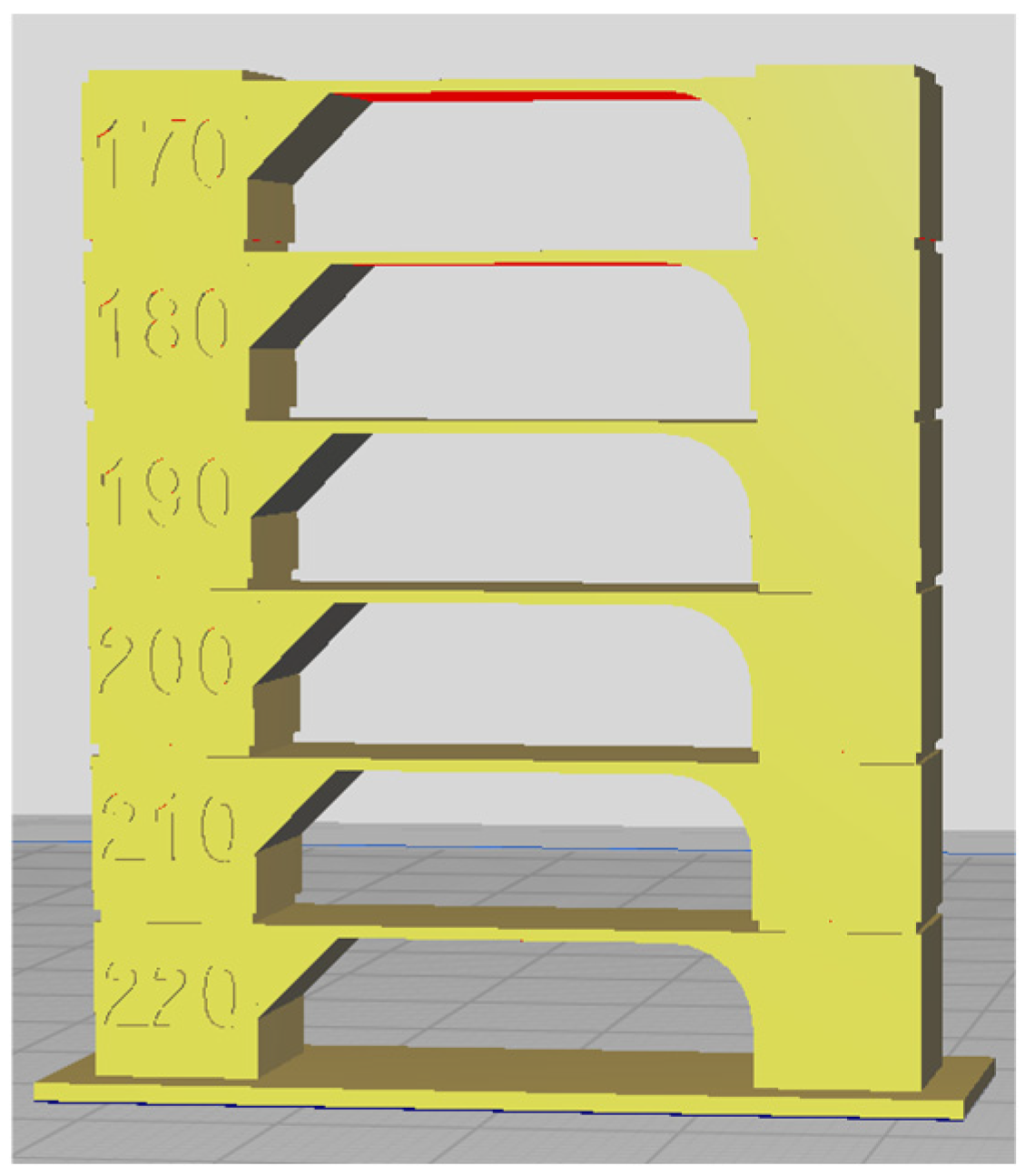
Figure 1.
Temperature tower for optimal 3D printing temperature determination—slicer-designed model for 3D printing.
Figure 1.
Temperature tower for optimal 3D printing temperature determination—slicer-designed model for 3D printing.
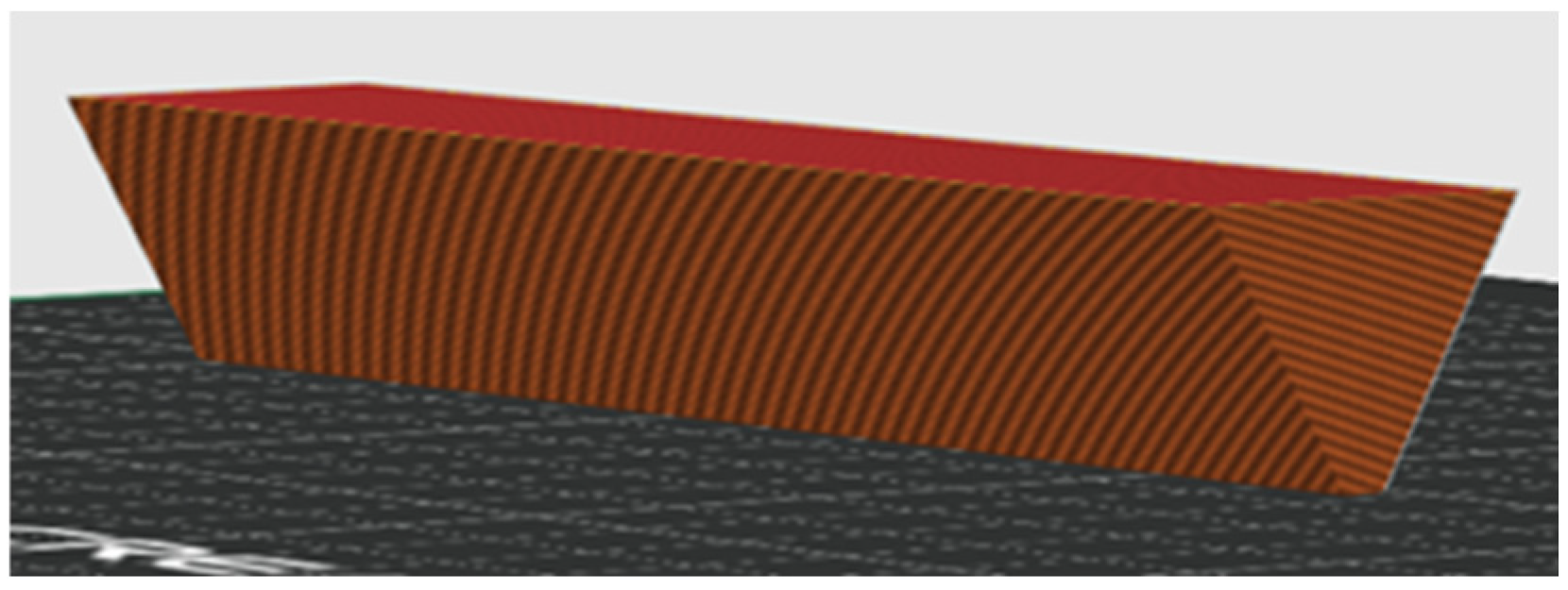
Figure 2.
Triangular prism for warping test A—slicer model for 3D printing.
Figure 2.
Triangular prism for warping test A—slicer model for 3D printing.
Figure 3.
(a) Slicer models of 3D-printed samples in square and rectangular shape from (a) top view and (b) side view (to show increase in thickness) and (c–e) conditions for composting test according to experiment arrangement.
Figure 3.
(a) Slicer models of 3D-printed samples in square and rectangular shape from (a) top view and (b) side view (to show increase in thickness) and (c–e) conditions for composting test according to experiment arrangement.
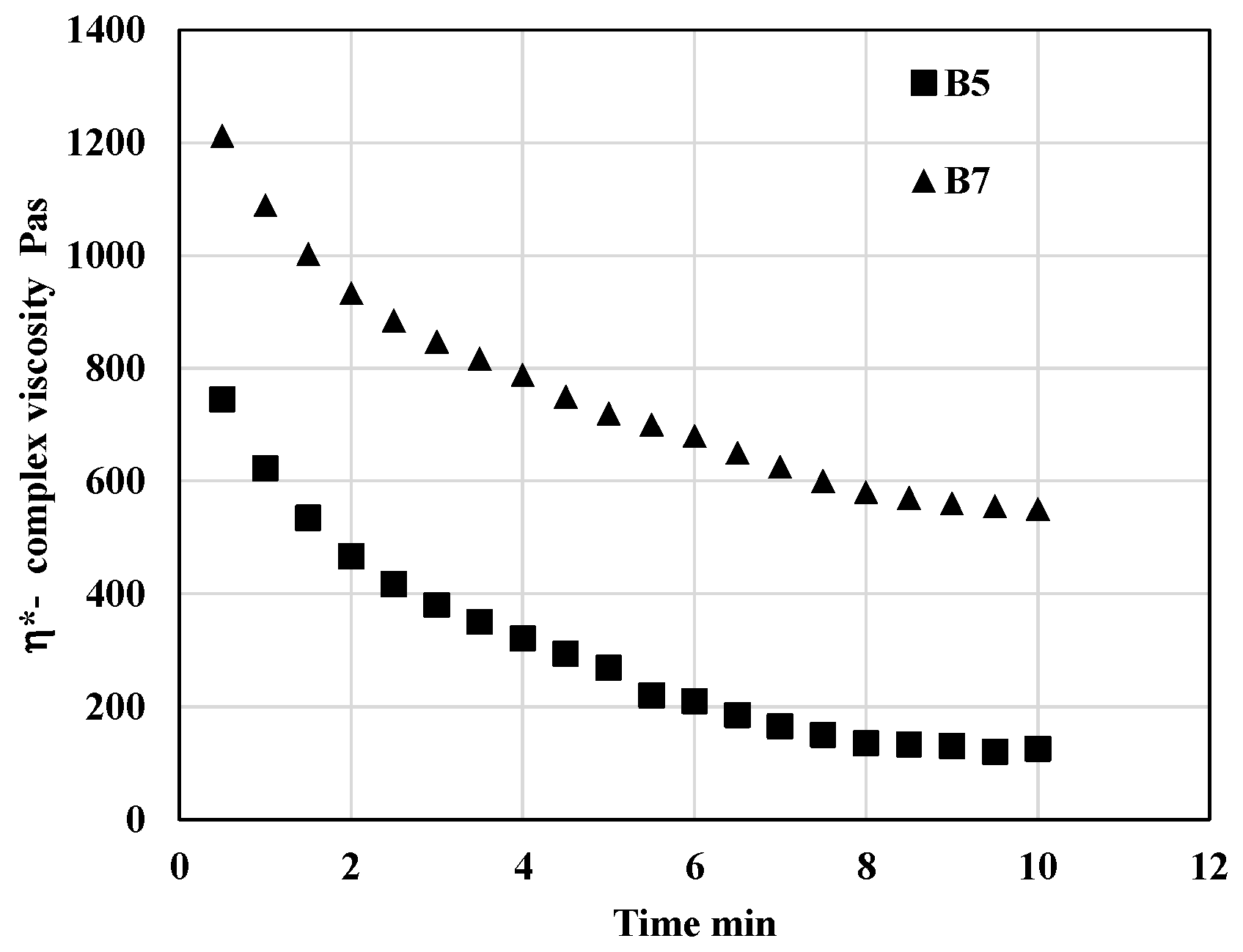
Figure 4.
Typical flow curves of prepared blends expressed in terms of the dependency of the (a) complex viscosity, (b) plastic part of viscosity, and (c) elastic part of viscosity at 160 °C for PLA, B5, and B7 blends.
Figure 4.
Typical flow curves of prepared blends expressed in terms of the dependency of the (a) complex viscosity, (b) plastic part of viscosity, and (c) elastic part of viscosity at 160 °C for PLA, B5, and B7 blends.
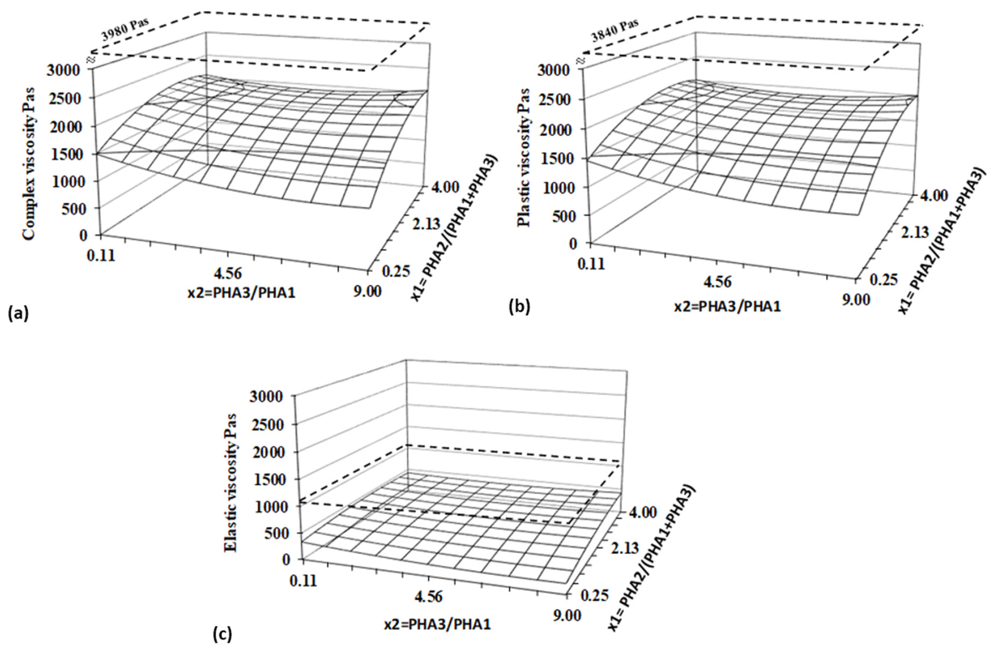
Figure 5.
Response surfaces for (a) complex, (b) elastic, and (c) plastic viscosity evaluated for a shear rate of 15 s−1 and a temperature of 160 °C. Dashed planes represent values for PLA.
Figure 5.
Response surfaces for (a) complex, (b) elastic, and (c) plastic viscosity evaluated for a shear rate of 15 s−1 and a temperature of 160 °C. Dashed planes represent values for PLA.
Figure 6.
Dependency of complex viscosity on time during thermo-mechanical loading in oscillatory rheometer at 200 °C.
Figure 6.
Dependency of complex viscosity on time during thermo-mechanical loading in oscillatory rheometer at 200 °C.
Figure 7.
Response surfaces for complex viscosity after 4 min of thermo-mechanical loading of blend in oscillatory rheometer at 200 °C. The results of the regression and statistical analysis indicate that the ratio of the two crystalline PHAs (PHA3/PHA1) has a significant effect on degradation during processing at the printing temperature. Specifically, a higher proportion of PHA1 (corresponding to a lower value of the x2 factor) leads to a markedly more stable blend compared to those with a higher content of PHA3. In contrast, the concentration of the amorphous PHA2 appears to have a negligible influence on the processing stability of the studied PHA-based blends. Despite the noticeable effect of blend composition on degradation at 200 °C, all formulations were successfully processed using 3D printing. This is attributed to the short exposure time to elevated temperature during printing, typically on the order of seconds, which was insufficient to allow significant thermal degradation to occur.
![Polymers 17 01477 g007]()
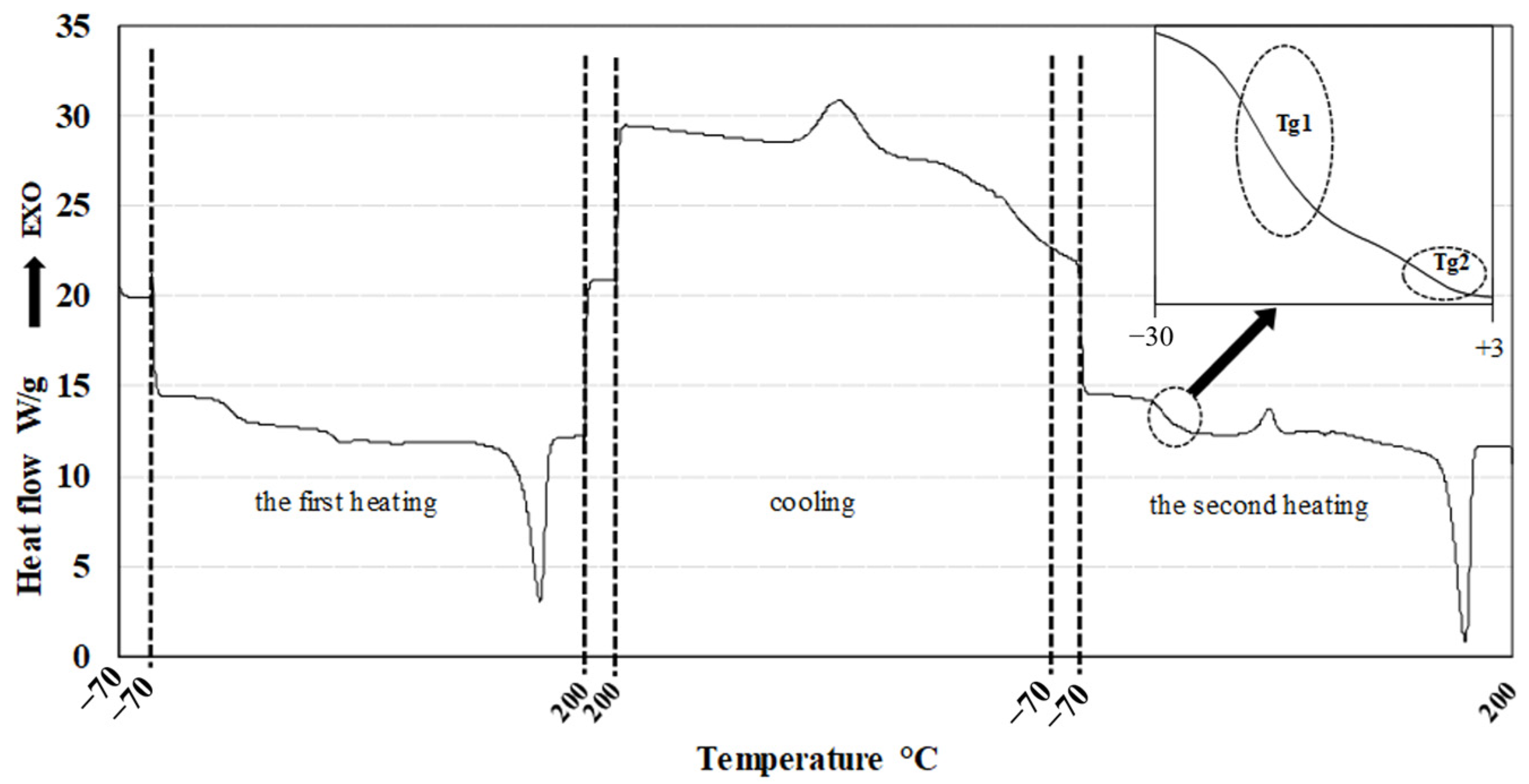
Figure 8.
Typical DSC record of PHA blends.
Figure 8.
Typical DSC record of PHA blends.
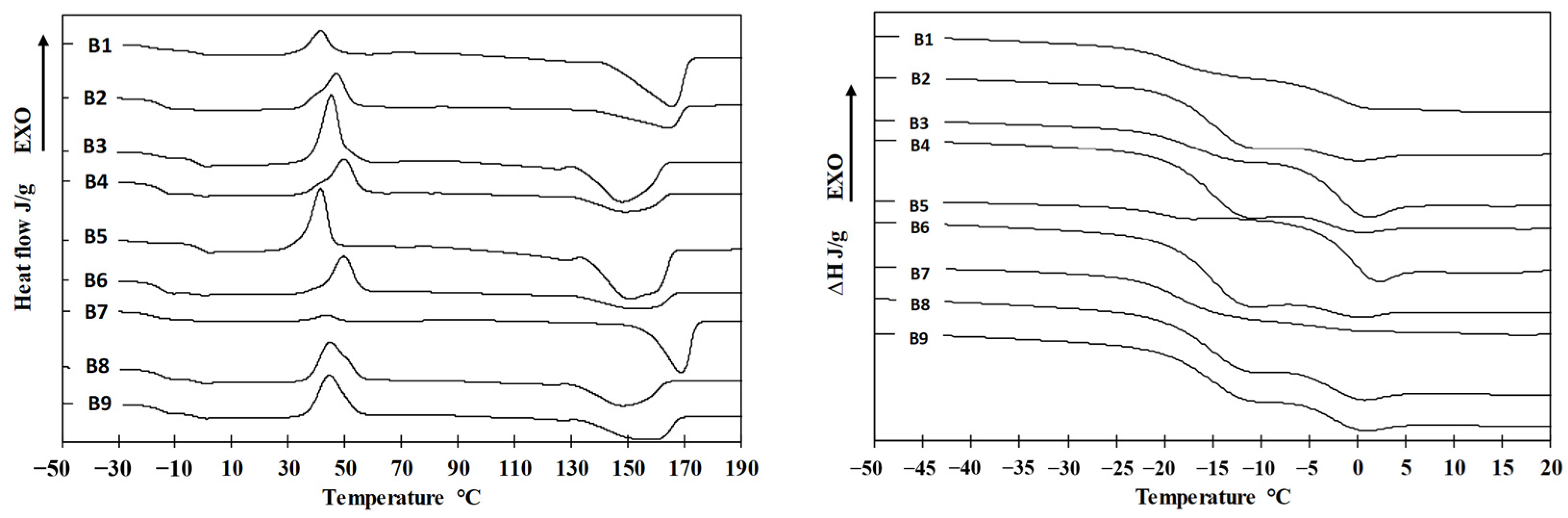
Figure 9.
Overall DSC 2nd heating records (left side) and magnification for Tg region (right side) for blends B1–B9.
Figure 9.
Overall DSC 2nd heating records (left side) and magnification for Tg region (right side) for blends B1–B9.
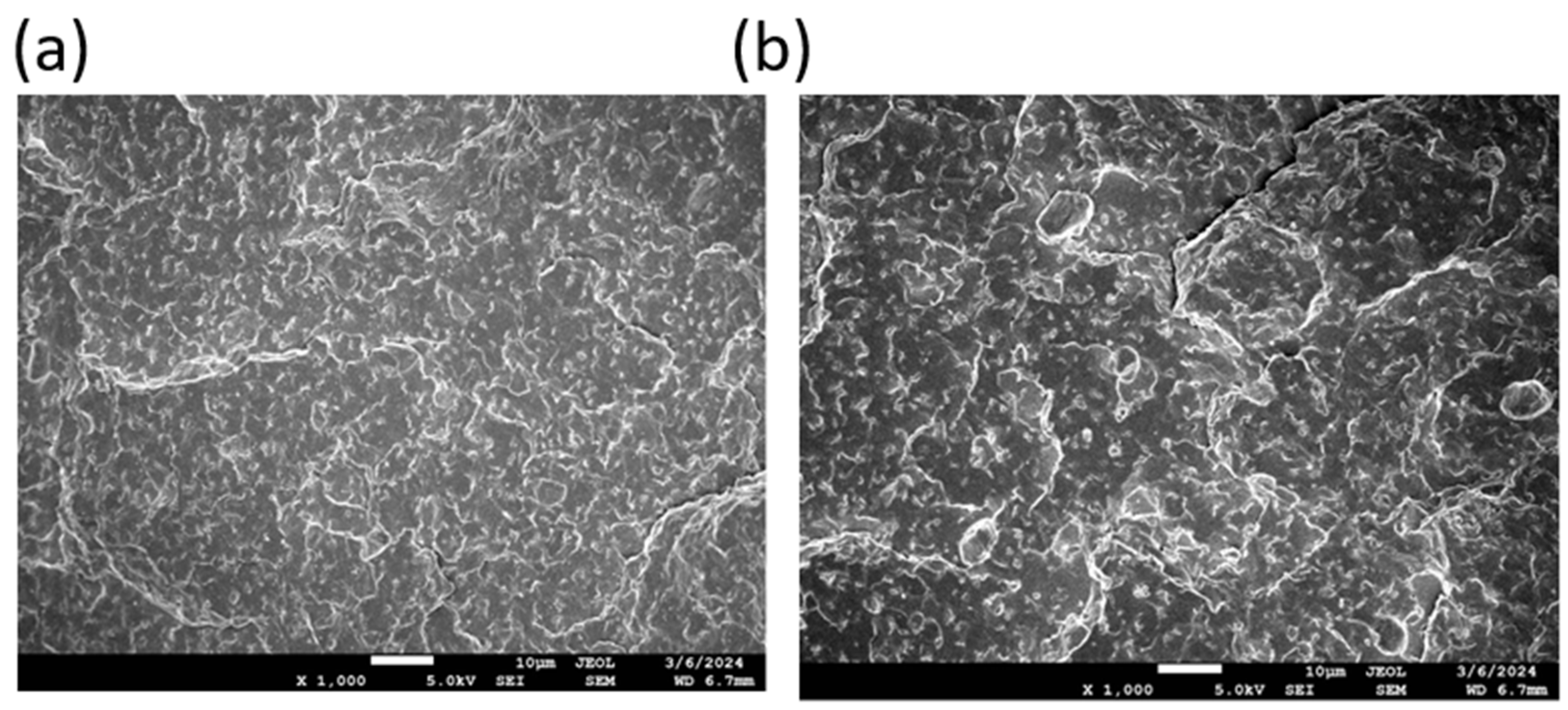
Figure 10.
SEM photos of (a) for the samples B1)= and (b) for the sample B2, showing the fracture surface of filaments at 1000× magnification.
Figure 10.
SEM photos of (a) for the samples B1)= and (b) for the sample B2, showing the fracture surface of filaments at 1000× magnification.
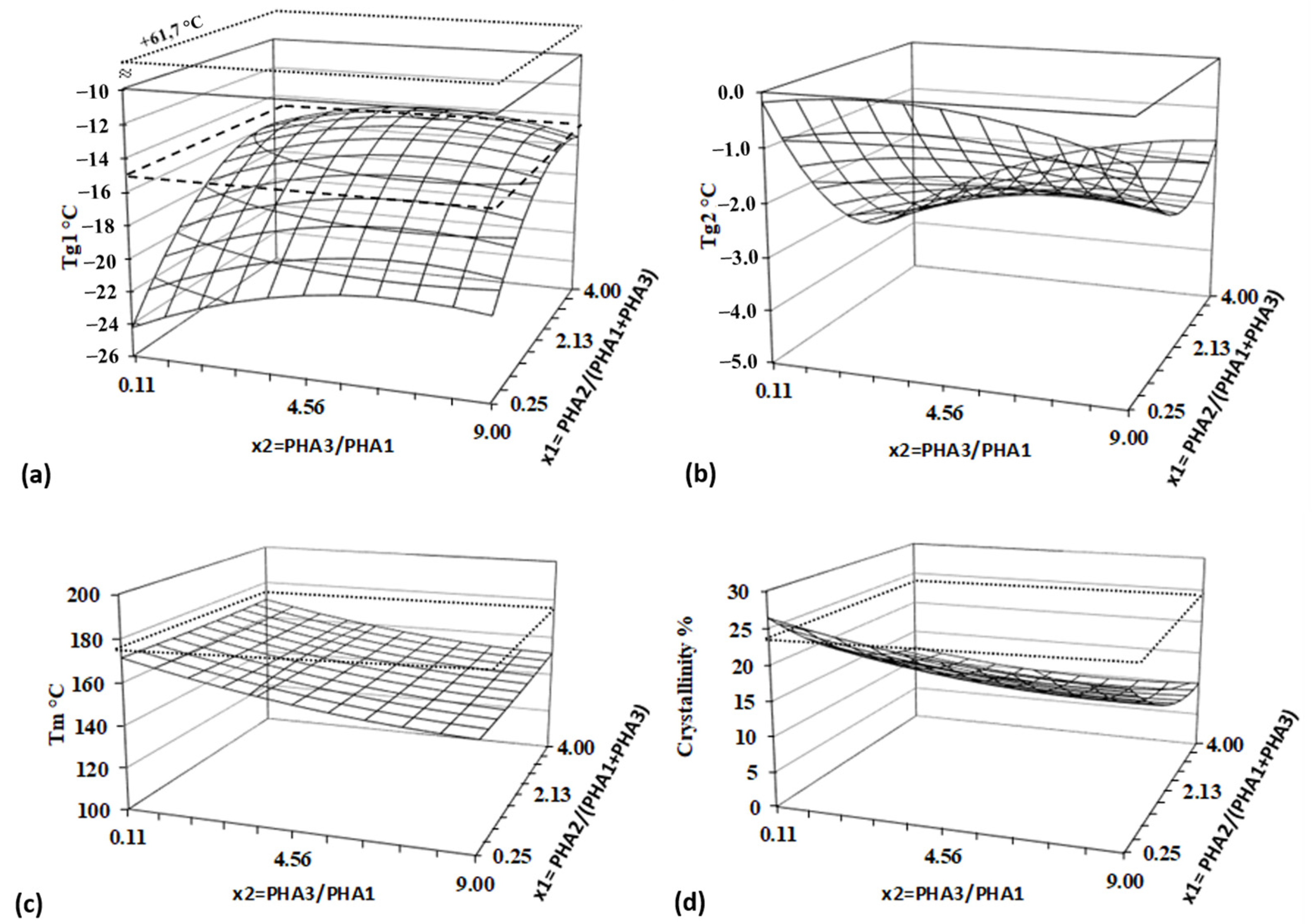
Figure 11.
Response surfaces for thermal properties and crystallinity—(a) lower Tg 1, (b) higher Tg, (c) melting temperature, and (d) crystallinity. Dashed line represents value for PHA2, and dotted lines represent values for PLA. Regression and statistical analysis of the Tg values further confirm strong physical interactions between PHA polymers in the blend. A significant non-linear deviation from the original Tg of PHA2 (−14.9 °C) is observed for Tg1, which originally belongs to PHA2. Additionally, the two Tg values corresponding to PHA1 (+5.1 °C) and PHA3 (+2.4 °C) disappear from the DSC curves, replaced by a single Tg2, which does not exceed 0 °C.
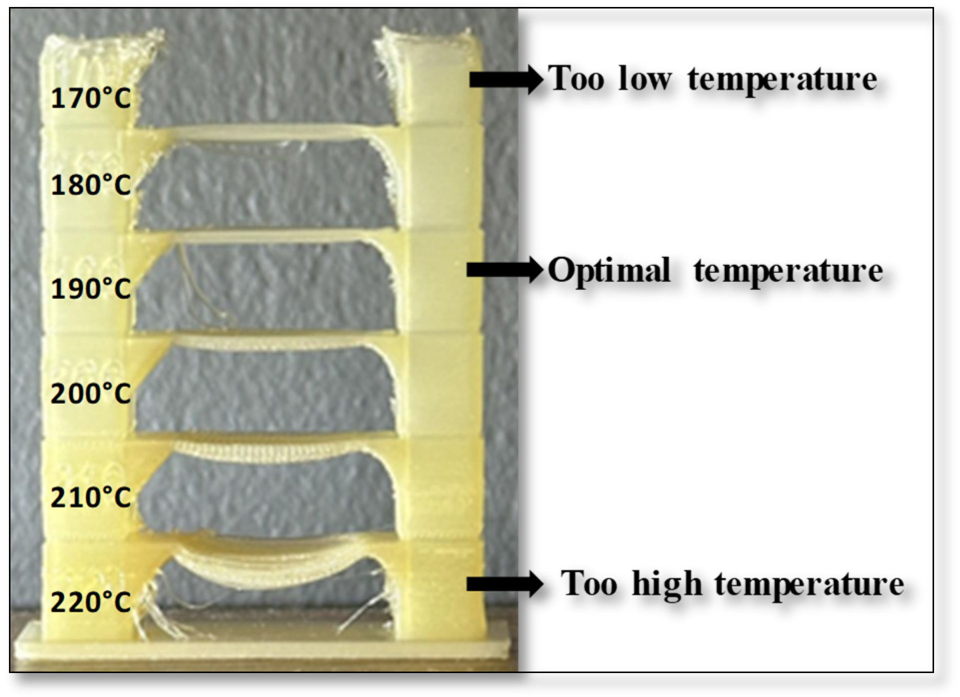
Figure 12.
The 3D-printed temperature tower for sample B8 in temperature range from 170 °C to 220 °C.
Figure 12.
The 3D-printed temperature tower for sample B8 in temperature range from 170 °C to 220 °C.
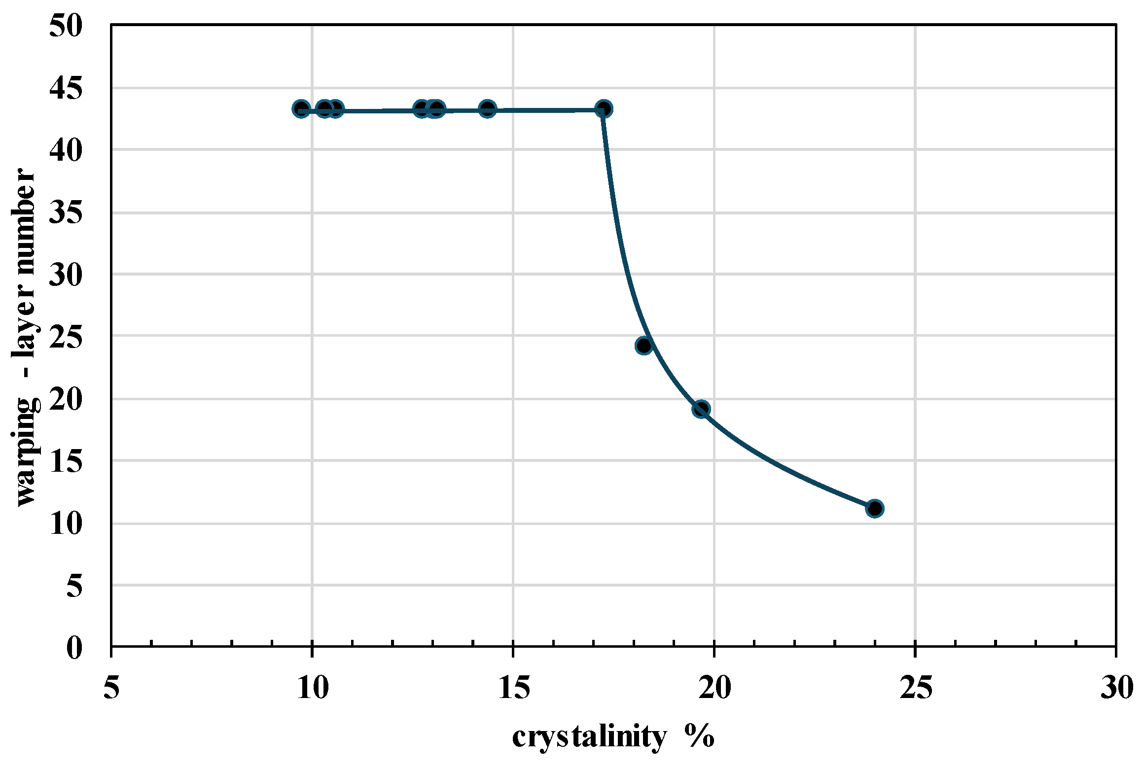
Figure 13.
Dependency of warping effect expressed as layer number when detachment from bed appears on crystallinity. Value 43 for the warping layer number indicates no warping effect.
Figure 13.
Dependency of warping effect expressed as layer number when detachment from bed appears on crystallinity. Value 43 for the warping layer number indicates no warping effect.
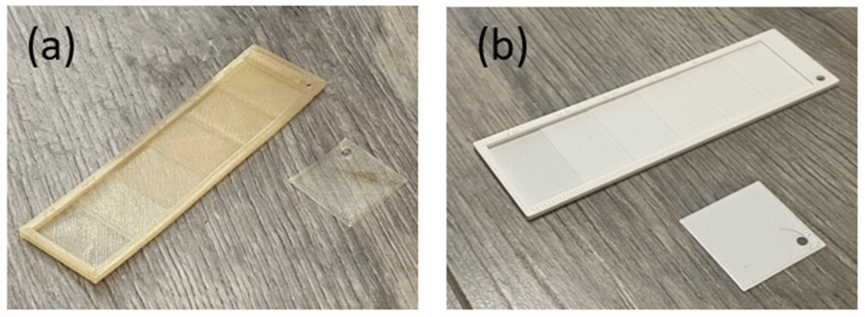
Figure 14.
Typical structure of FDM 3D-printed (a) PHA-based blends (for sample B8) and (b) PLA sample in rectangular stair-shaped design.
Figure 14.
Typical structure of FDM 3D-printed (a) PHA-based blends (for sample B8) and (b) PLA sample in rectangular stair-shaped design.
Figure 15.
Response surfaces for tensile properties measured on 3D filaments (left side); (a) young modulus, (c) yield strength, (e) tensile strength at break, (g) elongation at break and on 3D-printed specimens (right side), (b) young modulus, (d) yield strength, (f) tensile strength at break. Dashed lines represent values for PLA.
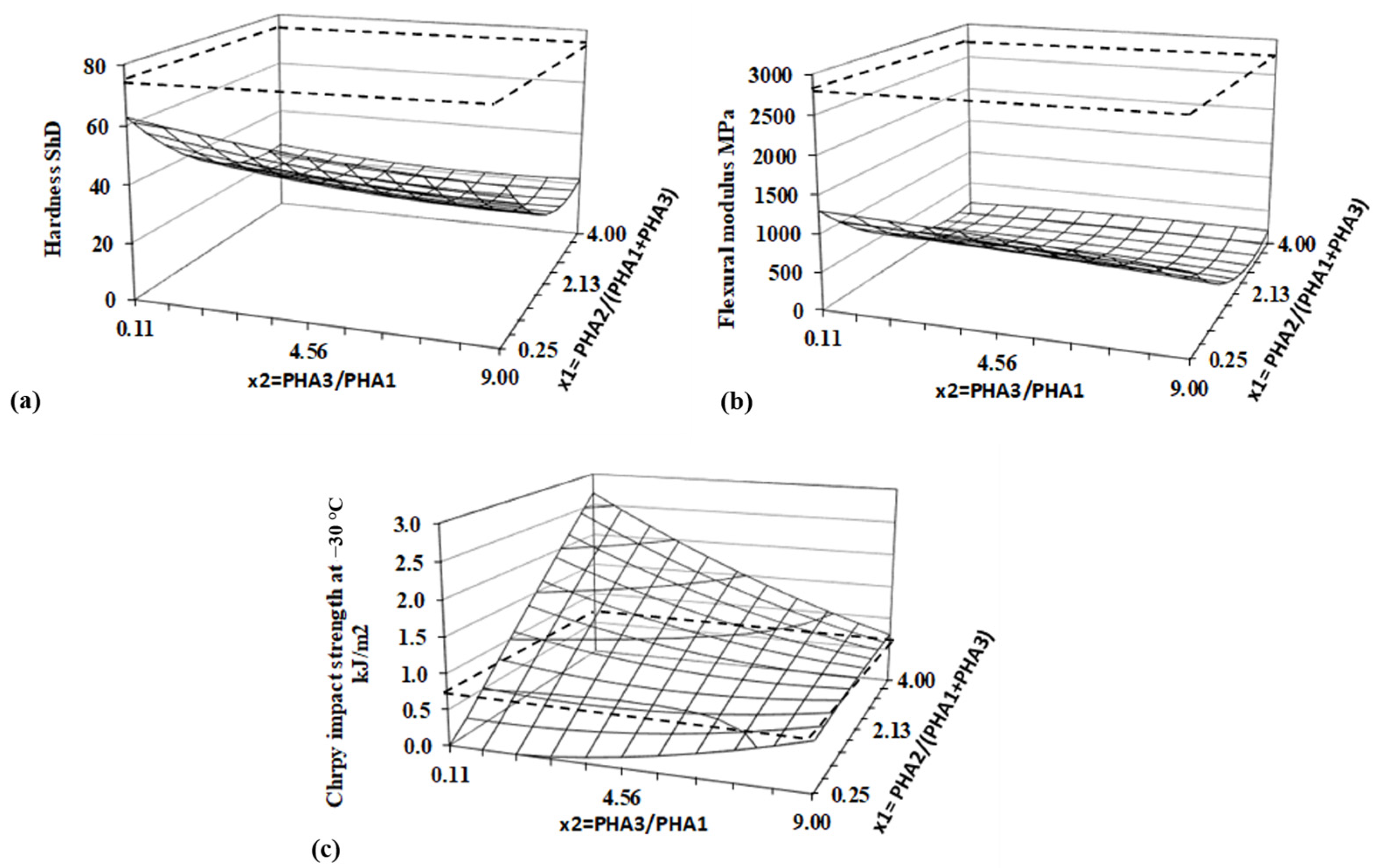
Figure 16.
Response surfaces for (a) hardness, (b) flexural modulus, and (c) impact strength. Dashed lines represent values for PLA.
Figure 16.
Response surfaces for (a) hardness, (b) flexural modulus, and (c) impact strength. Dashed lines represent values for PLA.
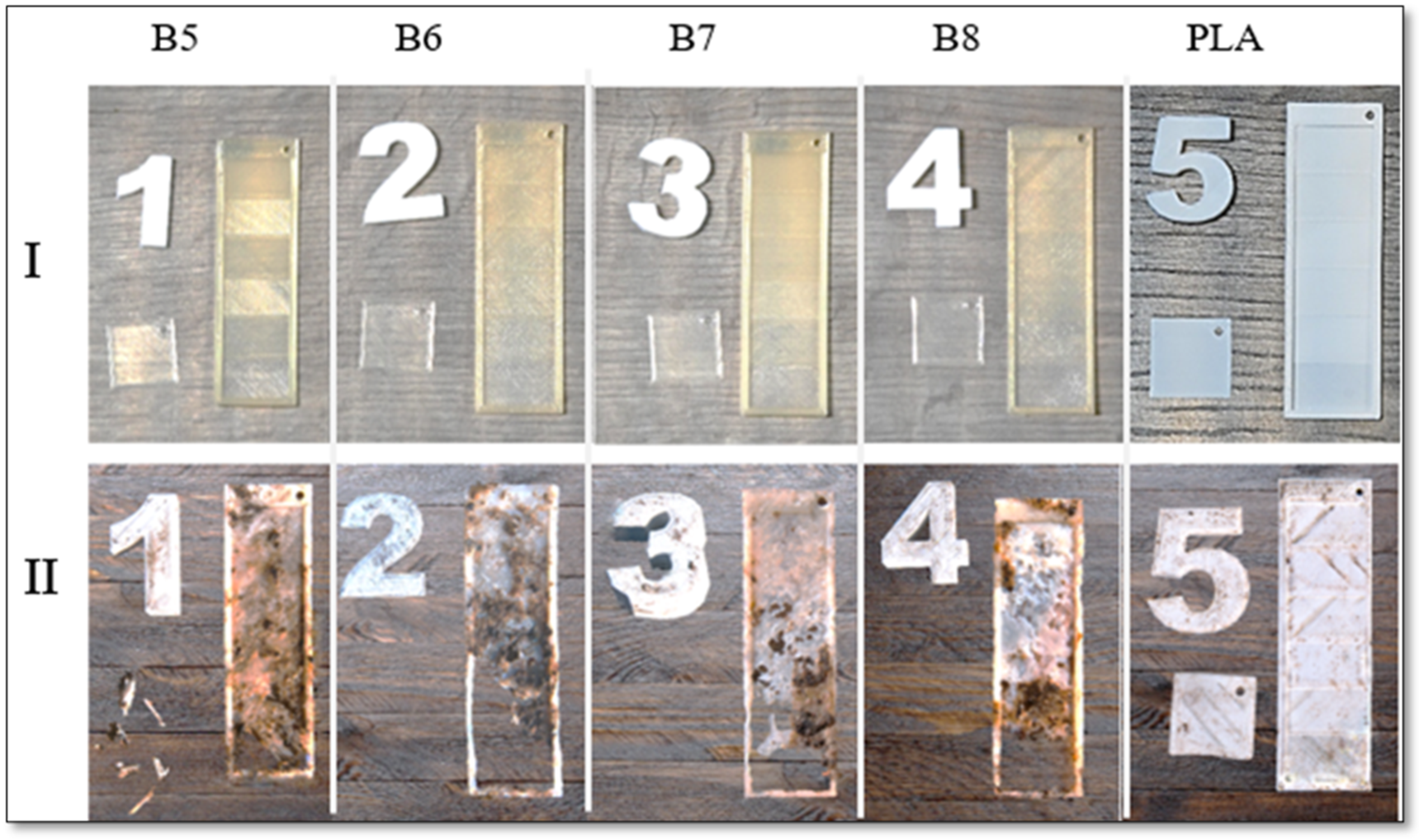
Figure 17.
Visual inspection of composting of 3D-printed samples: (I) before composting and (II) after 2 months of home composting for samples of B5, B6, B7, B8, and PLA with crystallinity values of 24.1, 10.4, 18.3. 13.1, and 25%, respectively.
Figure 17.
Visual inspection of composting of 3D-printed samples: (I) before composting and (II) after 2 months of home composting for samples of B5, B6, B7, B8, and PLA with crystallinity values of 24.1, 10.4, 18.3. 13.1, and 25%, respectively.
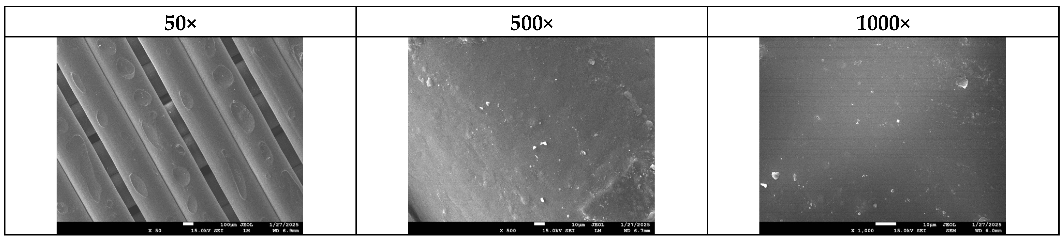
Figure 18.
Typical SEM photos of surfaces of sample B5 before composting in different magnifications.
Figure 18.
Typical SEM photos of surfaces of sample B5 before composting in different magnifications.
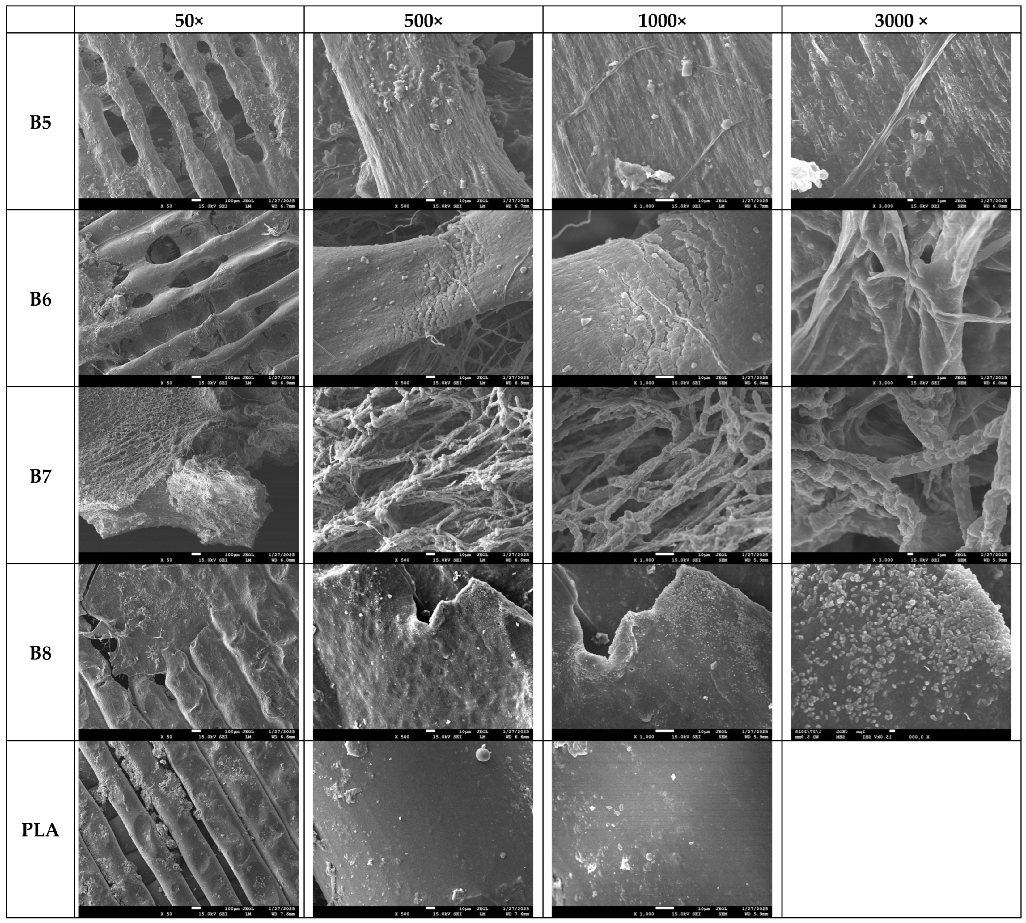
Figure 19.
SEM photos of surfaces of samples B5–B8 and PLA after composting (the magnification is given in the first row).
Figure 19.
SEM photos of surfaces of samples B5–B8 and PLA after composting (the magnification is given in the first row).
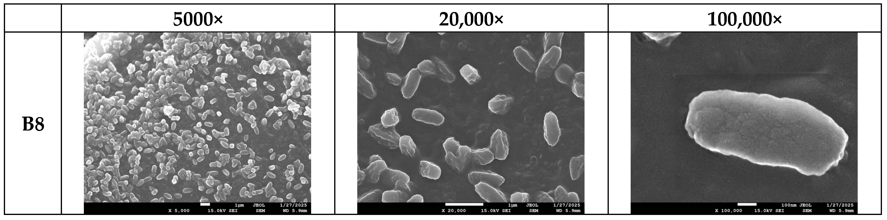
Figure 20.
SEM photos for identification of bacteria colony on sample B8’s surface in different magnifications (the magnification is given above the photo).
Figure 20.
SEM photos for identification of bacteria colony on sample B8’s surface in different magnifications (the magnification is given above the photo).
Figure 21.
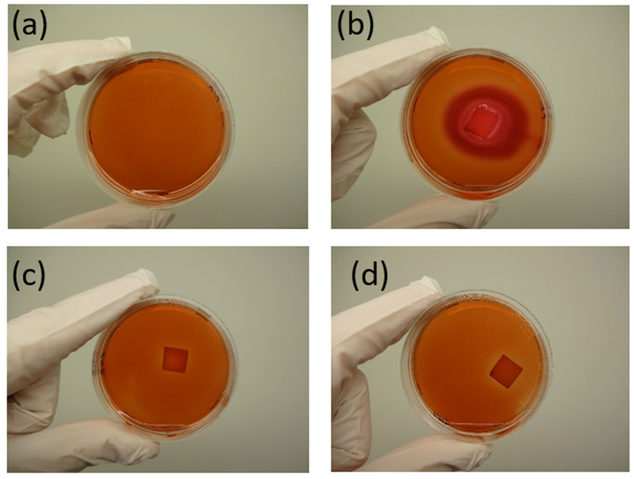
Results of the agar diffusion test for sample B5. (a) Negative control (only cells) (A (0/0), (b) positive control (gauze moistened with SDS) (B (4/4)), (c) sample B5 (C (0/0)), and (d) sample B8 (D (0/0)). The response index (zone/lysis) is indicated in parentheses.
Figure 21.
Results of the agar diffusion test for sample B5. (a) Negative control (only cells) (A (0/0), (b) positive control (gauze moistened with SDS) (B (4/4)), (c) sample B5 (C (0/0)), and (d) sample B8 (D (0/0)). The response index (zone/lysis) is indicated in parentheses.
Figure 22.
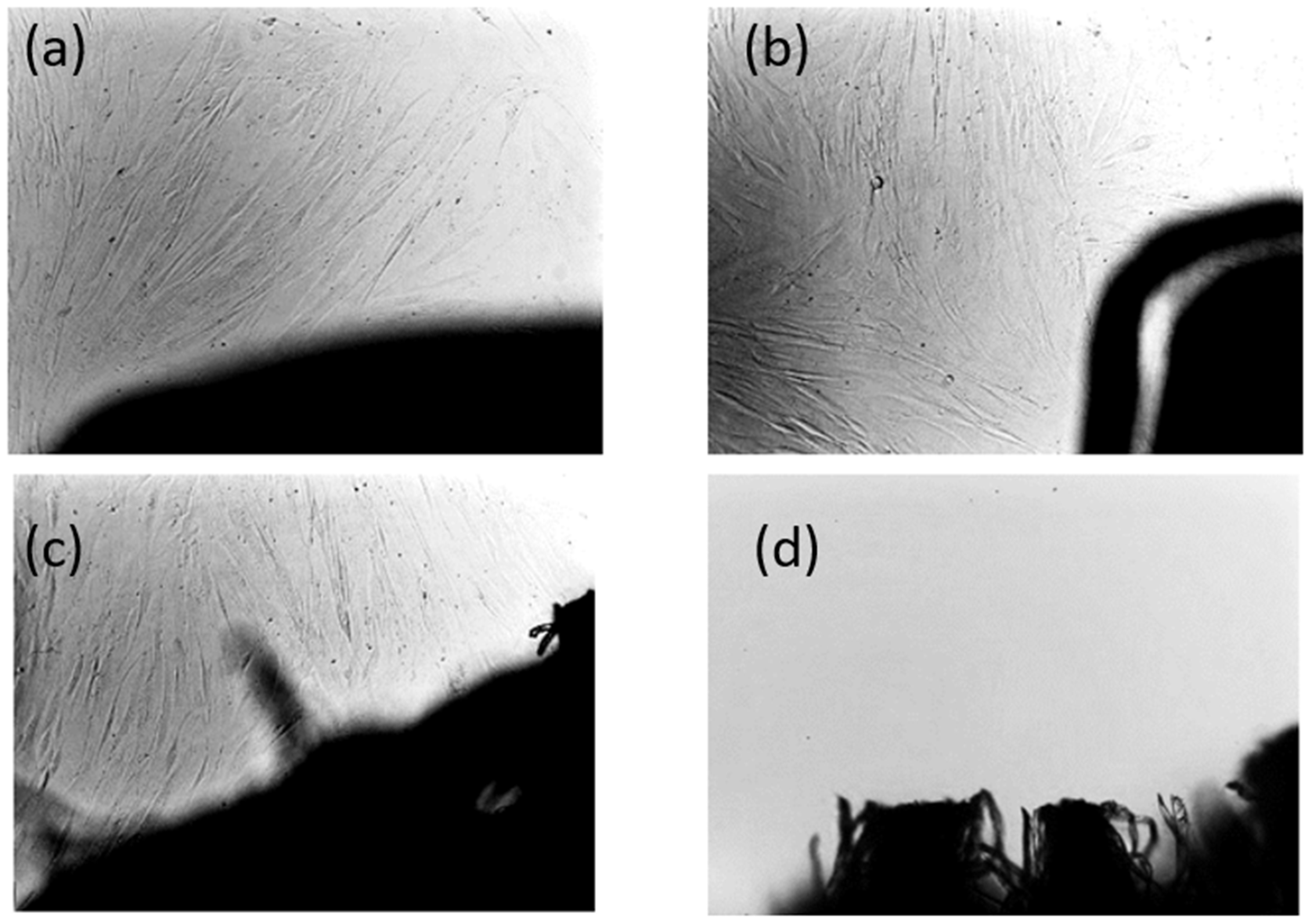
Microscopic images of cells cultivated in the presence of samples B5 (a) and B8 (b), alongside negative ((c)—gauze) and positive ((d)—gauze moistened with SDS) controls, after 72 h of the in vitro contact toxicity test (Magnification 10×).
Figure 22.
Microscopic images of cells cultivated in the presence of samples B5 (a) and B8 (b), alongside negative ((c)—gauze) and positive ((d)—gauze moistened with SDS) controls, after 72 h of the in vitro contact toxicity test (Magnification 10×).
Figure 23.
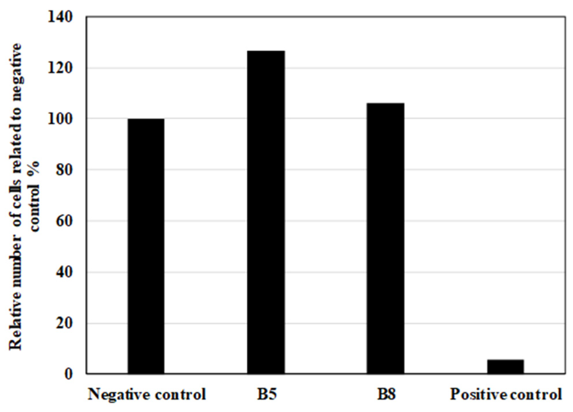
Cell proliferation after 72 h of in vitro contact toxicity test expressed in relative number (%) related to negative control with sterile gauze (100%).
Figure 23.
Cell proliferation after 72 h of in vitro contact toxicity test expressed in relative number (%) related to negative control with sterile gauze (100%).
Table 1.
Conditions of experiment.
Table 1.
Conditions of experiment.
| | Coded Levels | | | | | | |
|---|
| | −1.141 | −1 | 0 | 1 | 1.414 | | |
| Factor | Real values | | | | | Central value | step |
| x1 | 0.25 | 0.80 | 2.13 | 3.45 | 4 | 2.13 | 1.33 |
| x2 | 0.11 | 1.412 | 4.56 | 7.70 | 9 | 4.56 | 3.14 |
Table 2.
Composition of the blends in the DoE experiment.
Table 2.
Composition of the blends in the DoE experiment.
| Samples | Coded Values | Real Values |
|---|
| x1 | x2 | x1 | x2 |
|---|
| PHA2/(PHA1+PHA3) | PHA3/PHA1 | PHA2/(PHA1+PHA3) | PHA3/PHA1 |
|---|
| B1 | −1 | −1 | 0.80 | 1.412 |
| B2 | +1 | −1 | 3.45 | 1.412 |
| B2 | −1 | +1 | 0.80 | 7.7 |
| B4 | +1 | +1 | 3.45 | 7.7 |
| B5 | −1.414 | 0 | 0.25 | 4.56 |
| B6 | +1.414 | 0 | 4 | 4.56 |
| B7 | 0 | −1.414 | 2.13 | 0.11 |
| B8 | 0 | +1.414 | 2.13 | 9 |
| B9 | 0 | 0 | 2.13 | 4.56 |
| B10 | 0 | 0 | 2.13 | 4.56 |
| B11 | 0 | 0 | 2.13 | 4.56 |
| B12 | 0 | 0 | 2.13 | 4.56 |
| B13 | 0 | 0 | 2.13 | 4.56 |
Table 3.
Regression and statistical parameters evaluated for viscosity. (Values significant at 95% probability (α=0.05) are in bold.)
Table 3.
Regression and statistical parameters evaluated for viscosity. (Values significant at 95% probability (α=0.05) are in bold.)
| | Fcrit 0.05 | Complex Viscosity | Plastic Viscosity | Elastic Viscosity |
|---|
| F1 | 6.9 | 88.5 | 91.2 | 52.8 |
| F2 | 6.6 | 23.0 | 23.4 | 18.5 |
| FLF | 6.6 | 1.0 | 1.0 | 0.9 |
| | sE+/− | 62 | 59 | 17 |
| | sLF+/− | 61 | 60 | 16 |
| | b0 | 1817 | 1781 | 361 |
| | b1 | 278 | 272 | 55 |
| | b2 | −81 | −77 | −25 |
| | b11 | −160 | −156 | −34 |
| | b12 | 54 | 51 | 18 |
| | b22 | 81 | 77 | 25 |
Table 4.
Regression and statistical parameters evaluated for complex viscosity in 4th minute. (Values significant at 95% probability (α = 0.05) are in bold).
Table 4.
Regression and statistical parameters evaluated for complex viscosity in 4th minute. (Values significant at 95% probability (α = 0.05) are in bold).
| | Fcrit 0.05 | Complex Viscosity in 4th min |
|---|
| F1 | 6.9 | 121.4 |
| F2 | 6.6 | 76.7 |
| FLF | 6.6 | 22.7 |
| | sE+/− | 18.2 |
| | sLF+/− | 22.7 |
| | b0 | 366.8 |
| | b1 | 2.9 |
| | b2 | −100.4 |
| | b11 | −21.8 |
| | b12 | 32.3 |
| | b22 | 95.9 |
Table 5.
Tg, Tm, ΔHm, and crystallinity values of prepared blends and their components.
Table 5.
Tg, Tm, ΔHm, and crystallinity values of prepared blends and their components.
| Sample | Tg 1 (°C) | Tg 2 (°C) | Tm (°C) | ΔHm (J/g) | 1 Crystallinity (%) |
|---|
| PHA1 | 5.1 | - | 166.7 | 75.9 | 52.0 |
| PHA2 | −14.9 | - | - | - | - |
| PHA3 | 2.4 | - | 148.6 | 52.8 | 36.2 |
| B1 | −19.7 | −1.1 | 166.3 | 28.9 | 19.8 |
| B2 | −14.2 | −2.7 | 165.4 | 15.5 | 10.6 |
| B3 | −18.6 | −1.7 | 151.2 | 25.3 | 17.3 |
| B4 | −14.5 | −2.1 | 151.2 | 14.3 | 9.8 |
| B5 | −21.7 | 0.3 | 156.9 | 35.1 | 24.07 |
| B6 | −14.6 | −2.6 | 157.3 | 15.1 | 10.4 |
| B7 | −18.9 | −3.4 | 170.4 | 26.7 | 18.3 |
| B8 | −15.7 | −2.1 | 149.9 | 19.1 | 13.1 |
| B9 | −14.5 | −1.3 | 157.8 | 19.1 | 13.1 |
| B10 | −15.2 | −2.4 | 153.3 | 18.7 | 12.8 |
| B11 | −15.6 | −2.6 | 163.0 | 21.1 | 14.4 |
| B12 | −15.2 | −2.6 | 155.7 | 19.2 | 13.1 |
| B13 | −15.6 | −2.8 | 153.2 | 19.2 | 13.1 |
| PLA ref. | 61.16 | - | 151.8 | 23.4 | 25.0 |
Table 6.
Regression and statistical parameters evaluated for thermal properties and crystallinity. Values significant at 95% probability (α = 0.05) are in bold.
Table 6.
Regression and statistical parameters evaluated for thermal properties and crystallinity. Values significant at 95% probability (α = 0.05) are in bold.
| | Fcrit 0.05 | Tg1 | Tg2 | Tm | Crystallinity |
|---|
| F1 | 6.9 | 154.72 | 154.72 | 12.36 | 212.69 |
| F2 | 6.6 | 26.51 | 26.51 | 0.48 | 13.35 |
| FLF | 6.6 | 7.17 | 7.17 | 0.01 | 9.43 |
| | sE+/− | 0.41 | 0.41 | 4.1 | 0.64 |
| | sLF+/− | 1.10 | 1.10 | 0.4 | 1.98 |
| | b0 | −15.24 | −15.24 | 156.6 | 13.31 |
| | b1 | 2.46 | 2.46 | 0.0 | −4.50 |
| | b2 | 0.68 | 0.68 | −7.1 | −1.33 |
| | b11 | −1.20 | −1.20 | 0.3 | 1.43 |
| | b12 | −0.34 | −0.34 | 0.3 | 0.41 |
| | b22 | −0.79 | −0.79 | 1.8 | 0.67 |
Table 7.
Values of optimal printing temperature as well as values of warping effect.
Table 7.
Values of optimal printing temperature as well as values of warping effect.
| | Warping | Optimal Printing Temperature |
|---|
| Sample | (Layer Number) | (°C) |
|---|
| B1 | 19 | 200 |
| B2 | 43 | 200 |
| B3 | 43 | 200 |
| B4 | 43 | 205 |
| B5 | 11 | 200 |
| B6 | 43 | 210 |
| B7 | 24 | 200 |
| B8 | 43 | 200 |
| B9 | 43 | 200 |
| B10 | 43 | 200 |
| B11 | 43 | 205 |
| B12 | 43 | 200 |
| B13 | 43 | 205 |
| PLA | 43 | 210 |
Table 8.
Regression and statistical parameters evaluated for tensile properties of 3D filaments and 3D-printed specimens. Values significant at 95% probability (α = 0.05) are in bold.
Table 8.
Regression and statistical parameters evaluated for tensile properties of 3D filaments and 3D-printed specimens. Values significant at 95% probability (α = 0.05) are in bold.
| | | 3D Filaments | 3D-Printed Specimens |
|---|
| | Fcrit 0.05 | σY
1 | σB
2 | εB
3 | σY | σB | εB |
|---|
| F1 | 6.9 | 260.6 | 26.7 | 30.9 | 230.6 | 170.8 | 2.9 |
| F2 | 6.6 | 49.5 | 4.6 | 5.1 | 42.6 | 76.2 | 0.6 |
| FLF | 6.6 | 7.4 | 8.5 | 0.4 | 2.1 | 95.9 | 0.5 |
| | sE+/− | 0.77 | 1.4 | 420 | 0.79 | 0.58 | 348 |
| | sLF+/− | 2.09 | 4.0 | 249 | 1.15 | 5.69 | 240 |
| | b0 | 9.89 | 14.0 | 2662 | 7.64 | 4.14 | 610 |
| | b1 | −6.20 | −3.5 | 1158 | −5.96 | −3.78 | 289 |
| | b2 | −0.02 | −0.2 | −142 | −0.30 | −0.35 | −60 |
| | b11 | 3.42 | 1.6 | −623 | 3.35 | 2.99 | −90 |
| | b12 | −1.00 | −1.1 | −8 | −0.17 | 0.72 | −44 |
| | b22 | −0.14 | −0.5 | −94 | 0.09 | −0.96 | 136 |
Table 9.
Regression and statistical parameters evaluated for hardness, flexural modulus, and impact strength according to the Charpy unnotched method at −30 °C. (Values significant at 95% probability (α=0.5) are in bold.)
Table 9.
Regression and statistical parameters evaluated for hardness, flexural modulus, and impact strength according to the Charpy unnotched method at −30 °C. (Values significant at 95% probability (α=0.5) are in bold.)
| | Fcrit 0.05 | Hardness | Flexural Modulus | Impact Strength at −30 °C |
|---|
| F1 | 6.9 | 210.2 | 367.0 | 43.1 |
| F2 | 6.6 | 29.3 | 79.6 | 6.3 |
| FLF | 6.6 | 3.4 | 11.8 | 3.3 |
| | sE+/− | 1.7 | 37 | 0.17 |
| | sLF+/− | 3.1 | 126 | 0.30 |
| | b0 | 26.6 | 290 | 0.89 |
| | b1 | −11.8 | −351 | 0.50 |
| | b2 | −41 | −0.22 | |
| | b11 | 5.9 | 210 | −0.02 |
| | b12 | 1.0 | 36 | −0.34 |
Table 10.
Selected samples for home compostability testing.
Table 10.
Selected samples for home compostability testing.
| Sample Number in Compost | Sample Number in DoE | Sample Description |
|---|
| 1 | B5 | Sample with the lowest PHA2 amorphous PHA content at medium PHA3/PHA1 ratio |
| 2 | B6 | Sample with the highest PHA2 amorphous PHA content at medium PHA3/PHA1 ratio |
| 3 | B7 | Sample with lowest PHA3/PHA1 ratio at medium PHA2 content |
| 4 | B8 | Sample with highest PHA3/PHA1 ratio at medium PHA2 content |
| 5 | PLA | Commercial PLA sample |


 ,
, 


