
Macroscopic Stress-Strain Response and Strain-Localization Behavior of Biopolymer-Treated Soil


Abstract

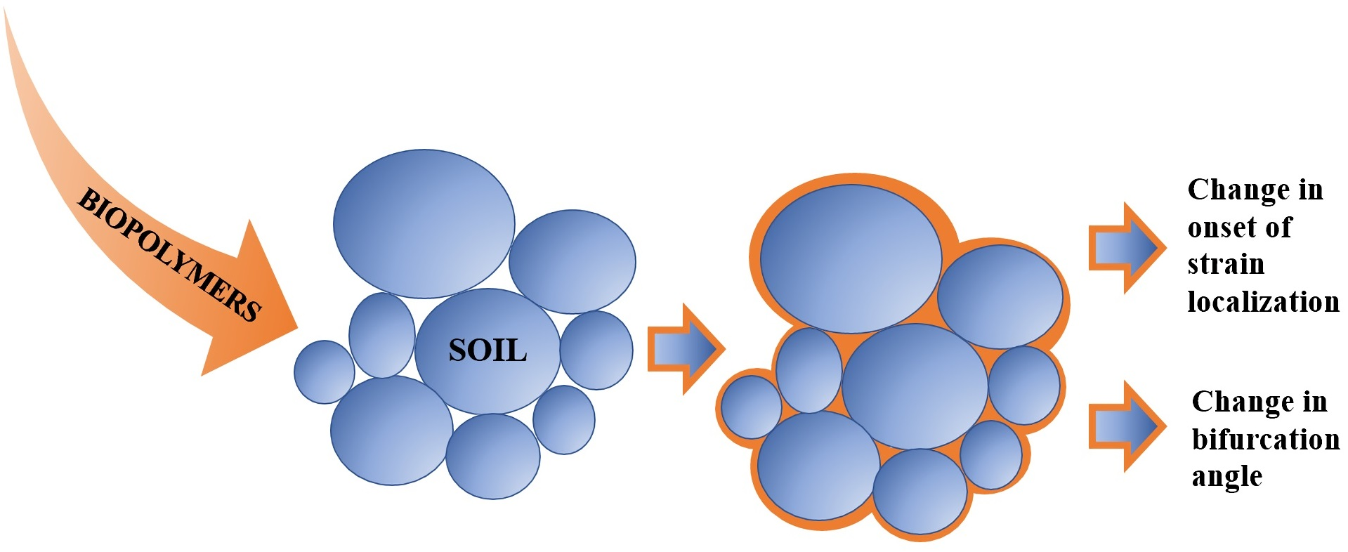
1. Introduction
2. Experimental Research
2.1. Soil
2.2. Biopolymers
2.2.1. Xanthan Gum
2.2.2. Guar Gum
2.2.3. Beta-Glucan
2.2.4. Specimen Preparation
2.2.5. Mechanical Testing
2.2.6. Digital Image Acquisition and Processing
3. Numerical Modeling
3.1. Stress-Strain Relationship
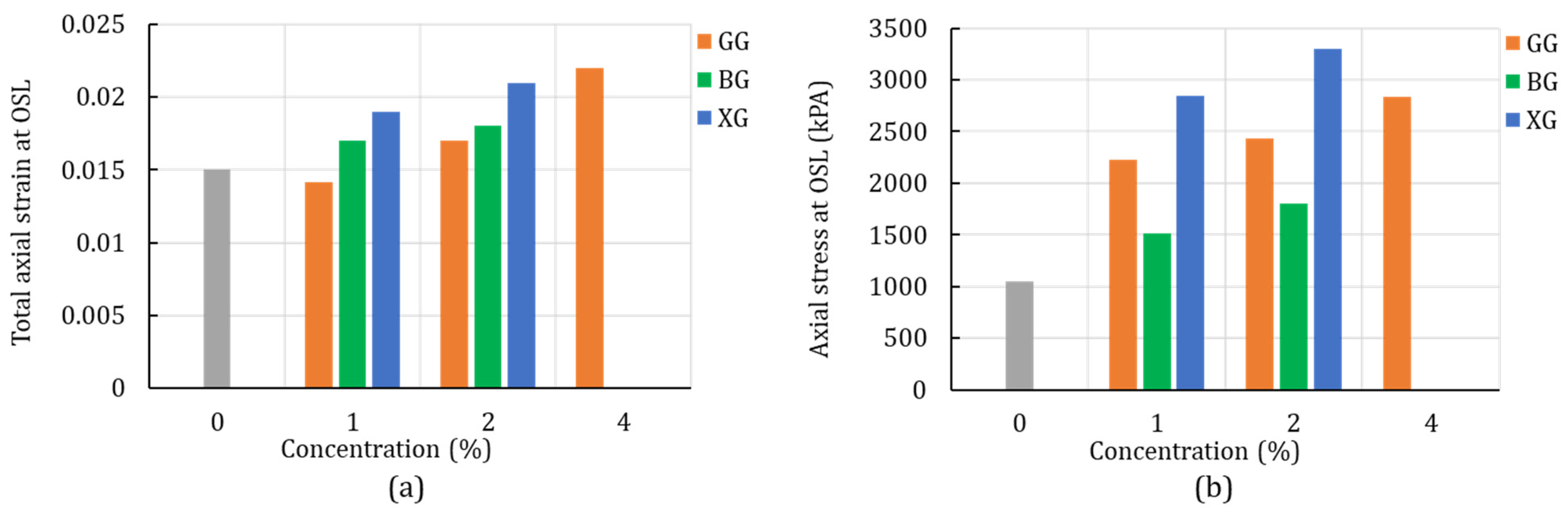
3.2. Onset of Strain Localization
3.3. Application to Drucker–Prager Model
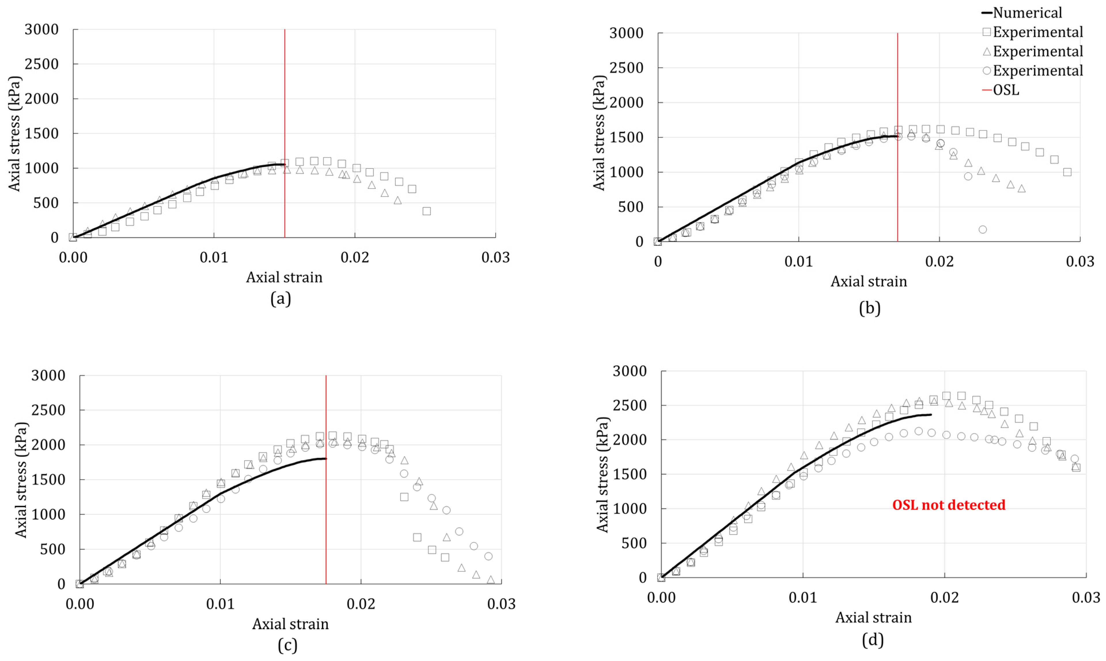
3.4. Numerical Simulation
3.5. Calibration of Constitutive Model
4. Results
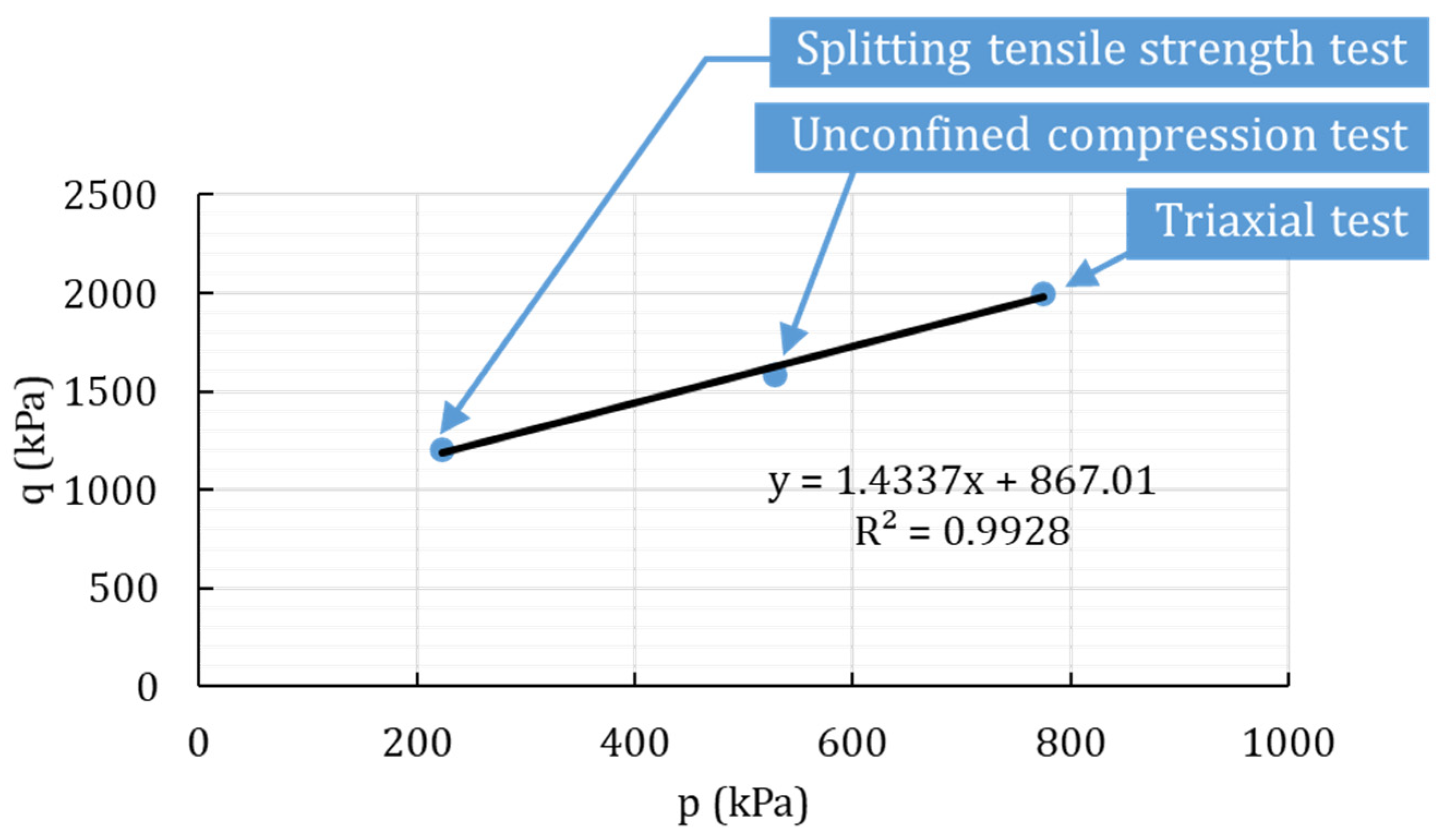
4.1. Unconfined Compression Test
4.2. Unconsolidated-Undrained Triaxial Test
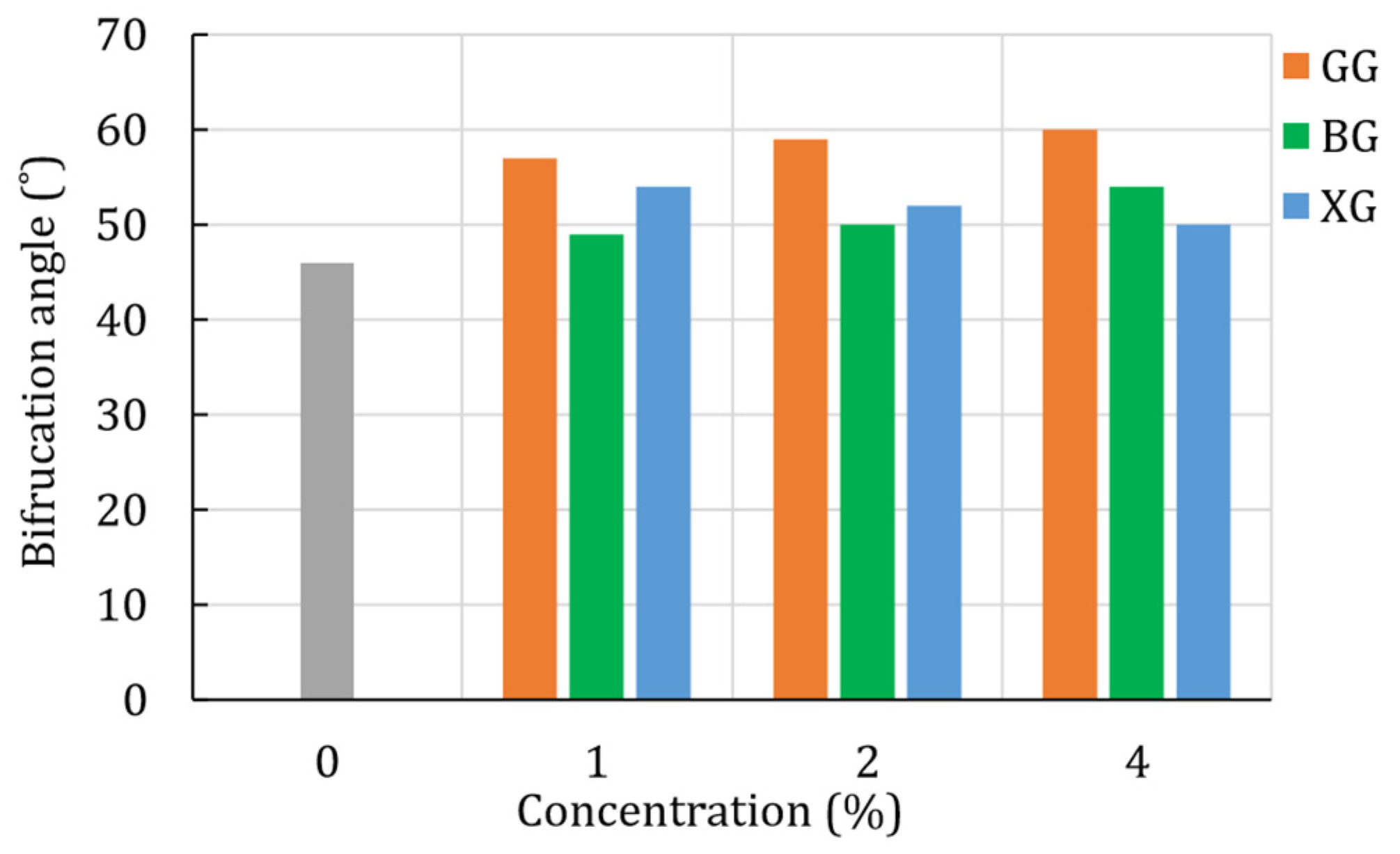
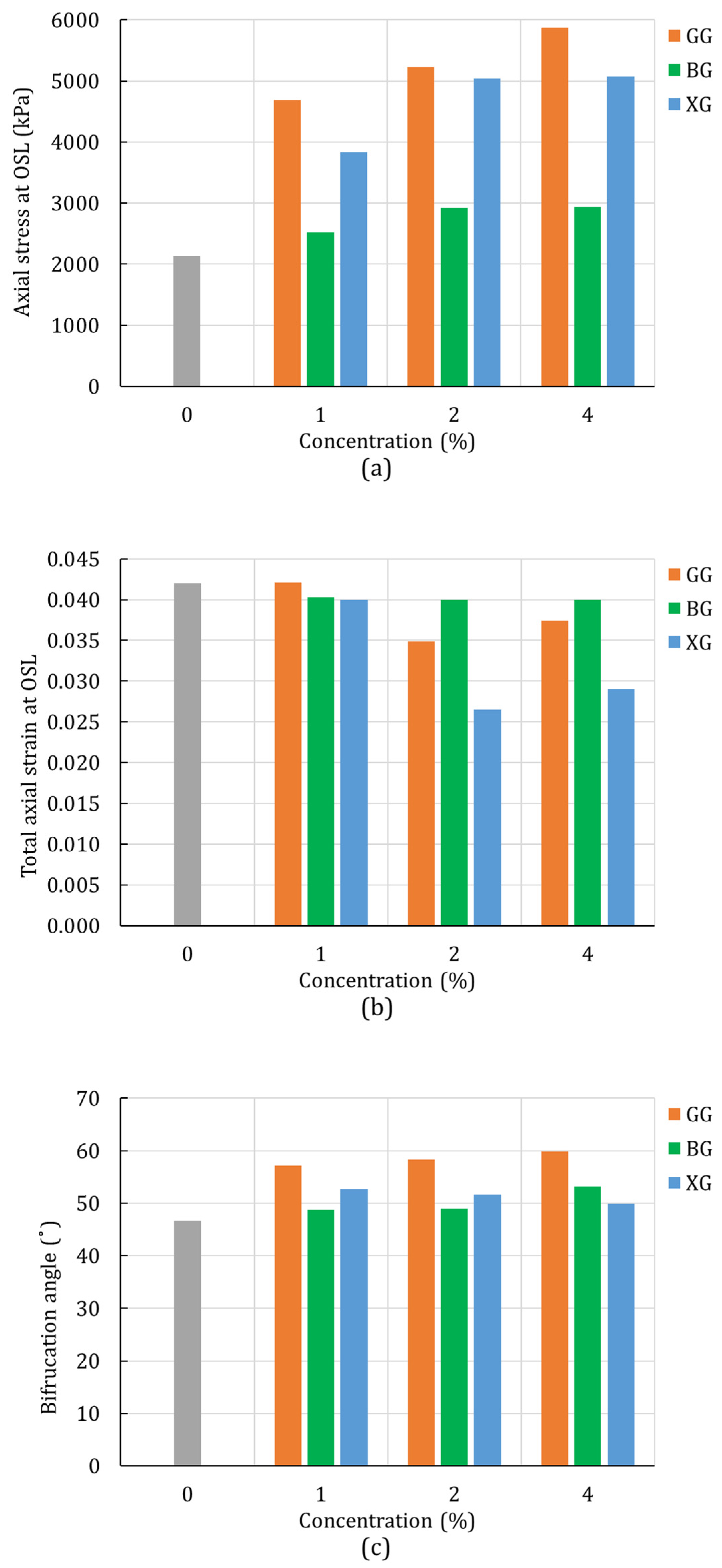
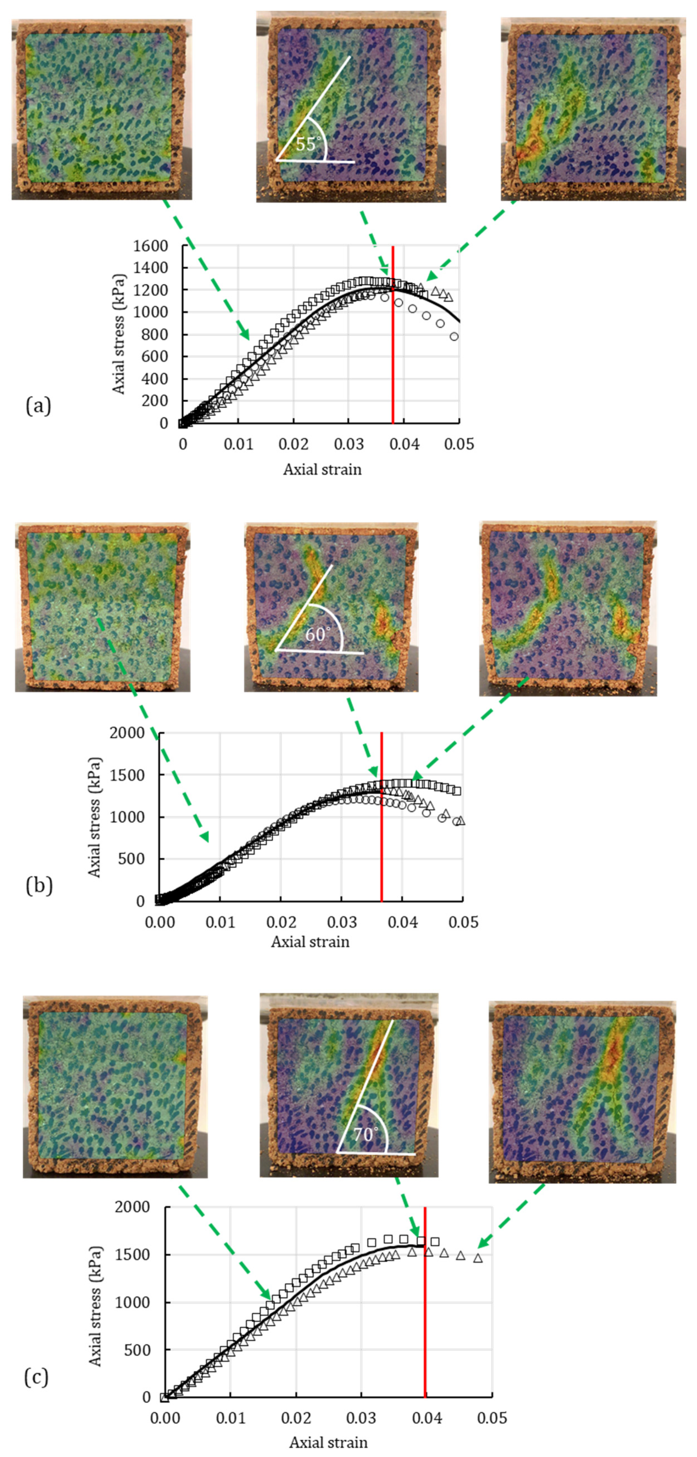
4.3. Digital Image Correlation
5. Conclusions
Author Contributions
Funding
Data Availability Statement
Conflicts of Interest
References
- Holtz, R.D.; Kovacs, W.D.; Thomas, C.; Sheahan, T.C. An Introduction to Geotechnical Engineering; Englewood Cliffs: Prentice-Hall, NJ, USA, 1981; Volume 733. [Google Scholar]
- Hinchee, R.E.; Lawrence, A.S. In Situ Thermal Technologies for Site Remediation; CRC Press: Boca Raton, FL, USA, 1992. [Google Scholar]
- Umar, M.; Kassim, K.A.; Ping Chiet, K.T. Biological process of soil improvement in civil engineering: A review. J. Rock Mech. Geotech. Eng. 2016, 8, 767–774. [Google Scholar] [CrossRef]
- Ashraf, M.S.; Azahar, S.B.; Yusof, N.Z. Soil Improvement Using MICP and Biopolymers: A Review. IOP Conf. Ser. Mater. Sci. Eng. 2017, 226, 012058. [Google Scholar] [CrossRef]
- Andrew, R.M. Global CO2 emissions from cement production. Earth Syst. Sci. Data 2018, 10, 195–217. [Google Scholar]
- DeJong, J.T.; Mortensen, B.M.; Martinez, B.C.; Nelson, D.C. Bio-mediated soil improvement. Ecol. Eng. 2010, 36, 197–210. [Google Scholar] [CrossRef]
- Chang, I.; Im, J.; Cho, G.-C. Introduction of Microbial Biopolymers in Soil Treatment for Future Environmentally-Friendly and Sustainable Geotechnical Engineering. Sustainability 2016, 8, 251. [Google Scholar] [CrossRef]
- Choi, S.-G.; Wang, K.; Chu, J. Properties of biocemented, fiber reinforced sand. Constr. Build. Mater. 2016, 120, 623–629. [Google Scholar] [CrossRef]
- Li, L.; Cetin, B.; Yang, X. Proceedings of the GeoShanghai 2018 International Conference: Ground Improvement and Geosynthetics; Springer: Berlin/Heidelberg, Germany, 2018. [Google Scholar]
- Katzbauer, B. Properties and applications of xanthan gum. Polym. Degrad. Stab. 1998, 59, 81–84. [Google Scholar] [CrossRef]
- Lee, K.Y.; Mooney, D.J. Alginate: Properties and biomedical applications. Prog. Polym. Sci. 2012, 37, 106–126. [Google Scholar] [CrossRef]
- Gombotz, W.R.; Wee, S.F. Protein release from alginate matrices. Adv. Drug Deliv. Rev. 2012, 64, 194–205. [Google Scholar] [CrossRef]
- Thombare, N.; Jha, U.; Mishra, S.; Siddiqui, M.Z. Guar gum as a promising starting material for diverse applications: A review. Int. J. Biol. Macromol. 2016, 88, 361–372. [Google Scholar] [CrossRef]
- Chang, I.; Im, J.; Prasidhi, A.K.; Cho, G.-C. Effects of Xanthan gum biopolymer on soil strengthening. Constr. Build. Mater. 2015, 74, 65–72. [Google Scholar] [CrossRef]
- Aguilar, R.; Nakamatsu, J.; Ramírez, E.; Elgegren, M.; Ayarza, J.; Kim, S.; Pando, M.A.; Ortega-San-Martin, L. The potential use of chitosan as a biopolymer additive for enhanced mechanical properties and water resistance of earthen construction. Constr. Build. Mater. 2016, 114, 625–637. [Google Scholar] [CrossRef]
- Ayeldeen, M.; Negm, A.; El-Sawwaf, M.; Kitazume, M. Enhancing mechanical behaviors of collapsible soil using two biopolymers. J. Rock Mech. Geotech. Eng. 2017, 9, 329–339. [Google Scholar] [CrossRef]
- Wiszniewski, M.; Skutnik, Z.; Biliniak, M.; Çabalar, A.F. Some geomechanical properties of a biopolymer treated medium sand. Ann. Wars. Univ. Life Sci.—SGGW. Land Reclam. 2017, 49, 201–212. [Google Scholar] [CrossRef]
- Cabalar, A.F.; Wiszniewski, M.; Skutnik, Z. Effects of Xanthan Gum Biopolymer on the Permeability, Odometer, Unconfined Compressive and Triaxial Shear Behavior of a Sand. Soil Mech. Found Eng. 2017, 54, 356–361. [Google Scholar] [CrossRef]
- Soldo, A.; Miletić, M. Study on Shear Strength of Xanthan Gum-Amended Soil. Sustainability 2019, 11, 6142. [Google Scholar] [CrossRef]
- Toufigh, V.; Kianfar, E. The effects of stabilizers on the thermal and the mechanical properties of rammed earth at various humidities and their environmental impacts. Constr. Build. Mater. 2019, 200, 616–629. [Google Scholar] [CrossRef]
- Soldo, A.; Miletić, M.; Auad, M.L. Biopolymers as a sustainable solution for the enhancement of soil mechanical properties. Sci. Rep. 2020, 10, 267. [Google Scholar] [CrossRef]
- Chen, R.; Ding, X.; Ramey, D.; Lee, I.; Zhang, L. Experimental and numerical investigation into surface strength of mine tailings after biopolymer stabilization. Acta Geotech. 2016, 11, 1075–1085. [Google Scholar] [CrossRef]
- ASTM D6913-17; Standard Test Methods for Particle-Size Distribution (Gradation) of Soils Using Sieve Analysis. ASTM International: West Conshohocken, PA, USA, 2017; pp. 1–34.
- ASTM D4318-17; Standard Test Methods for Liquid Limit, Plastic Limit, and Plasticity Index of Soils. ASTM International: West Conshohocken, PA, USA, 2017; pp. 1–20.
- Volman, J.J.; Ramakers, J.D.; Plat, J. Dietary modulation of immune function by β-glucans. Physiol. Behav. 2008, 94, 276–284. [Google Scholar] [CrossRef]
- Bacic, A.; Fincher, G.B.; Stone, B.A. Chemistry, Biochemistry, and Biology of 1–3 Beta Glucans and Related Polysaccharides; Academic Press: Cambridge, MA, USA, 2009. [Google Scholar]
- ASTM D2166/D2166M-16; Standard Test Method for Unconfined Compressive Strength of Cohesive Soil. ASTM International: West Conshohocken, PA, USA, 2016; pp. 1–7.
- ASTM D2850-15; Standard Test Method for Unconsolidated-Undrained Triaxial Compression Test on Cohesive Soils. ASTM International: West Conshohocken, PA, USA, 2015; pp. 1–7.
- ASTM D3967-16; Standard Test Method for Splitting Tensile strength of Intact Rock Core Specimens. ASTM International: West Conshohocken, PA, USA, 2016; pp. 1–5.
- Akin, D.I.; Likos, W.J. Brazilian Tensile Strength Testing of Compacted Clay. Geotech. Test. J. 2017, 40, 20160180. [Google Scholar] [CrossRef]
- Gom Correlate. Zeiss. Braunschweig, Germany. 2019. Available online: https://www.zeiss.co.jp/metrology/magajin/2021/gom-inspect-suite.html (accessed on 2 January 2022).
- Miletić, M. Modeling of Localized Deformation in High and Ultra-High Performance Fiber Reinforced Cementitious Composites. Ph.D. Thesis, Kansas State University, Manhattan, Kansas, 2016. [Google Scholar]
- Miletić, M.; Perić, D. Effect of Fibers on the Onset of Strain Localization in HPFRCC Subjected to Plane Stress Loading. J. Eng. Mech. 2018, 144, 04018074. [Google Scholar] [CrossRef]
- Hirai, H.; Takahashi, M.; Yamada, M. An elastic-plastic constitutive model for the behavior of improved sandy soils. Soils Found. 1989, 29, 69–84. [Google Scholar] [CrossRef][Green Version]
- Rahimi, M.; Chan, D.; Nouri, A. Bounding surface constitutive model for cemented sand under monotonic loading. Int. J. Geomech. 2016, 16, 04015049. [Google Scholar] [CrossRef]
- Ottosen, N.S.; Runesson, K. Properties of discontinuous bifurcation solutions in elasto-plasticity. Int. J. Solids Struct. 1991, 27, 401–421. [Google Scholar] [CrossRef]
- Truty, A.; Obrzud, R. The Hardening Soil Model—A Practical Guidebook; Zace Services Ltd., Software Engineering: Lausanne, Switzerland, 2011. [Google Scholar]
- Chang, I.; Prasidhi, A.K.; Im, J.; Cho, G.-C. Soil strengthening using thermo-gelation biopolymers. Constr. Build. Mater. 2015, 77, 430–438. [Google Scholar] [CrossRef]
- Das, B.M. Advanced Soil Mechanics, 5th ed.; CRC Press: Boca Raton, FL, USA, 2019. [Google Scholar]
- Strömblad, N. Modeling of Soil and Structure Interaction Subsea. Master’s Thesis, Chalmers University of Technology, Göteborg, Sweden, 2014; p. 70. [Google Scholar]
- Schnaid, F.; Prietto, P.D.M.; Consoli, N.C. Characterization of Cemented Sand in Triaxial Compression. J. Geotech. Geoenviron. Eng. 2001, 127, 857–868. [Google Scholar] [CrossRef]
- Kutanaei, S.S.; Choobbasti, A.J. Triaxial behavior of fiber-reinforced cemented sand. J. Adhes. Sci. Technol. 2016, 30, 579–593. [Google Scholar] [CrossRef]
- Tagliaferri, F.; Waller, J.; Andò, E.; Hall, S.A.; Viggiani, G.; Bésuelle, P.; DeJong, J.T. Observing strain localisation processes in bio-cemented sand using X-ray imaging. Granul. Matter 2011, 13, 247–250. [Google Scholar] [CrossRef]


| Material | E (MPa) | β (°) | (°) | v |
|---|---|---|---|---|
| Plain soil | 88 | 34 | 1 | 0.3 |
| GG (1%) | 234 | 63 | 1 | 0.3 |
| GG (2%) | 217 | 64 | 1 | 0.3 |
| GG (4%) | 184 | 65 | 1 | 0.3 |
| BG (1%) | 114 | 42 | 1 | 0.3 |
| BG (2%) | 130 | 46 | 1 | 0.3 |
| BG (4%) | 162 | 55 | 1 | 0.3 |
| XG (1%) | 249 | 54 | 1 | 0.3 |
| XG (2%) | 243 | 51 | 1 | 0.3 |
| XG (4%) | 233 | 46 | 1 | 0.3 |
Publisher’s Note: MDPI stays neutral with regard to jurisdictional claims in published maps and institutional affiliations. |
© 2022 by the authors. Licensee MDPI, Basel, Switzerland. This article is an open access article distributed under the terms and conditions of the Creative Commons Attribution (CC BY) license (https://creativecommons.org/licenses/by/4.0/).
Share and Cite
Soldo, A.; Aguilar, V.; Miletić, M. Macroscopic Stress-Strain Response and Strain-Localization Behavior of Biopolymer-Treated Soil. Polymers 2022, 14, 997. https://doi.org/10.3390/polym14050997
Soldo A, Aguilar V, Miletić M. Macroscopic Stress-Strain Response and Strain-Localization Behavior of Biopolymer-Treated Soil. Polymers. 2022; 14(5):997. https://doi.org/10.3390/polym14050997
Chicago/Turabian StyleSoldo, Antonio, Victor Aguilar, and Marta Miletić. 2022. "Macroscopic Stress-Strain Response and Strain-Localization Behavior of Biopolymer-Treated Soil" Polymers 14, no. 5: 997. https://doi.org/10.3390/polym14050997
APA StyleSoldo, A., Aguilar, V., & Miletić, M. (2022). Macroscopic Stress-Strain Response and Strain-Localization Behavior of Biopolymer-Treated Soil. Polymers, 14(5), 997. https://doi.org/10.3390/polym14050997