Abstract
The control and prediction of morphological changes in annealed void microstructures is an essential and powerful tool for different semiconductor applications, for example, as part of the production of pressure sensors, resonators, or other silicon structures. In this work, with a focus on the void shape evolution of silicon, a novel simulation approach based on the level-set method is introduced to predict the continuous transformation of initial etched nano/micro-sized cylindrical structures at different annealing conditions. The developed model, which is based on a surface diffusion formulation and built in COMSOL Multiphysics® (Stockholm, Sweden), is introduced and compared to experimental literature data as well as with other analytical approaches. Some advantages of the presented model include the capability of simulating other materials under similar phenomena, the simulation of any possible initial geometry, and the visualization of intermediate steps during the annealing processing.
1. Introduction
Prediction and control of the evolution of void microstructures in silicon is a relevant topic in the semiconductor industry due to its wide range of applications such as being part of the production of pressure sensors [1], SON transistors [2,3,4], resonators [5,6], or even for microcooling [1]. All these applications have in common the prerequisite of generating a certain void cavity or empty space in silicon (ESS) below the main device structure or below a layer of silicon, i.e., a silicon-on-nothing (SON) layer. For this reason, simulations capable of reproducing the void formation are crucial to control the size and evolution of such structures.
Regarding the void generation, there exist different approaches such as lateral etching [2,7,8] or ion-implantation with optional annealing step [9,10]. In this work, the case study is focused on the SON technique, or void shape evolution process [11,12,13], which is based on a surface diffusion approach. The general method to obtain SON microstructures is as follows [11,13,14,15]: it starts generally with the etching of cylindrical cavities in silicon. After that, there is an annealing step at very high temperatures (1000–1100 °C), low pressures (about 10 Torr), and with a reducing ambient gas, such as hydrogen. After some minutes under these conditions, the initial cylindrical trench, due to surface diffusion phenomena and surface energy minimization, is separated from the external silicon layer and then it evolves until reaching an equilibrium geometry with the lowest surface energy possible, which is usually a spherical void. If several trenches are annealed within a close distance, then several spheres may coalescence forming a plate-shaped void, a technique that is also used for the “Silicon Millefeuille” process [16,17]. Both possibilities are shown in Figure 1. In this work, only the first case, the most frequent one, is investigated to verify the correctness of the simulated non-linear physics that will be described later when describing the model.
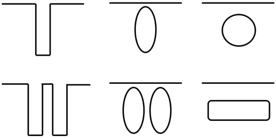
Figure 1.
Scheme of the SON process from trench to equilibrium sphere (top) and with coalescence from neighboring trenches to plate shape void (bottom).
Concerning the process controllability, it is more difficult to deal with the void shape evolution than, for instance, a direct lateral etching as there is no control between the initial and final structures. Consequently, the development of an effective and powerful simulation model that can represent the overall transformation at any annealing time becomes necessary. Recently, several models and simulation methods have been proposed. Initial solutions were based on the direct solving of the surface diffusion equations with some simplifications [14,18,19,20,21]. However, this is usually limited to some corner scenarios where the certain simplification is valid. The moving mesh method was also tested [22] and, while some results are similar to those in the literature, the method needs the definition of a virtual curvature function based on perturbation dynamics of cylindrical geometries. Therefore, the method can only simulate a few initial geometries. Moreover, due to the required large mesh elements, the moving mesh method requires a post-processing step to evaluate the obtained results. Phase field/level-set methods, by contrast, have been proven to deal well with two-phase and interface surface tension phenomena in fluid mechanics [23,24,25]. Furthermore, this method can simulate coalescence, which is an important step within the process. However, these models usually rely on volumetric phenomena to proceed with the simulations. Surface diffusion occurs, on the other hand, only at the interphase (gas–solid) with no effect of what occurs in the bulk of the material. Thus, in this work, a custom level-set formulation has been developed to adapt the features of the level-set method with the non-linear surface diffusion formulation of the void shape evolution of silicon. It is shown that this new approach can provide the evolution of the void morphology at any given processing time. Furthermore, all steps of the simulation procedure are described in detail.
The developed and presented custom level-set model in COMSOL Multiphysics® (version 5.1) can potentially be used with any initial geometry; it can be adapted to any material undergoing a similar surface diffusion process; and, with the combination of the already introduced analytical model for quick equilibrium estimations [26], it provides a powerful prediction and control void shape evolution toolbox. The proposed model is evaluated by means of the geometrical evolution, and simulated processing times are provided for reference. The simulated results are based on standard properties of isotropic intrinsic Si (100). However, the proposed material parameters were not fitted to match experimental data; they provide just a first estimation.
2. Materials and Methods
In this section, the equations used in the model are introduced. Firstly, the kinetic surface diffusion equation is shown as the most predominant phenomenon of the void shape evolution of silicon [14,27,28,29]. After that, a generalized level-set formulation is presented, followed by the coupling of both formulations and the boundary conditions of the simulations.
2.1. Kinetic Surface Diffusion Formulation
The movement of surface atoms undergoing a surface diffusion phenomenon is driven by the variation of the chemical potential from one atom of the surface to another neighboring one [30]. With GS as the Gibbs free energy of the surface and Ni as the atom of the ith species, the chemical potential μi is defined as
The Gibbs free energy of the surface corresponds to the surface energy of a solid, which is the required energy of formation to maintain the external shape of the molecules in a solid state. The surface energy is proportional to the surface size and thus its number of particles. In general, A being the surface area, and γ being the surface energy density, the Gibbs free energy of the surface yields [31,32,33]
Combining Equations (1) and (2), the chemical potential of the surface energy can be calculated as the variation of the Gibbs free surface energy per particle on the system. It can be demonstrated [30,32] that the discrete increase in surface area, δA, when an atom is added or removed from the system is given by
where K is the sum of the two main curvatures of the surface (local mean curvature) and Ω is the atomic volume. Accordingly, the local chemical potential of the surface is
The driving force that produces the movement of the surface atoms is defined by the variation of the chemical potential on the surface, i.e., the negative surface gradient, ∇S, of the chemical potential [14,30,34,35,36]:
Using the Nernst–Einstein relation [34] and assuming a Boltzmann distribution, the drift velocity of the surface particles, , is given by
where DS is the surface diffusion coefficient, kB is the Boltzmann constant, and T is the temperature. The atomic flux on the surface, jS, due to the drift velocity of the particles is the concentration of the particles on the surface, XS, multiplied by the drift velocity of those same particles:
Eventually, each atom on the surface moving from one point to another leaves a vacancy whose size corresponds to the atomic volume of the particle that left such position [34]. The resulting vacancies cause a normal displacement of the boundary surface proportional to the displaced atom. The normal velocity, vn, of the surface driven by surface diffusion can be continuously determined as follows:
This continuous equation is a general kinetic formulation of the motion of the interface due to surface diffusion, which results from the energy minimization of the surface. This equation describes the physics behind the simulation of the void shape evolution in silicon.
2.2. General Level-Set Method Formulation with Interface Reinitialization
The movement and tracking of the interface between silicon and the annealing gas is modelled, in this work, with the level-set method, due to its proven use in multiphase fluid mechanics simulation and its ability to effectively calculate the curvature of the interface between the two existing phases. Furthermore, it can potentially simulate coalescence, which is not tested in this work but can be useful for further extensions of the model. The standard method implemented in COMSOL Multiphysics® is explained below.
The level-set method is based on the advection equation of a certain so-called phase-field variable, ϕ, and a certain velocity field, v, [37,38,39]:
In this formulation, the level-set variable would evolve according to the defined velocity. The definition of the level-set variable is as follows [38]:
The initial conditions of the level-set variable, ϕ0, are defined by the parameter Dw, which is the distance to the interface, and ε, which is the interface thickness, in the so-called Heaviside function [24,38,40]. This is the formulation of a smooth interface transition at the surroundings of the surface layer, while staying almost constant in the bulk phase:
However, the pure advection shown in Equation (9) is highly unstable in simulations. Consequently, stabilization through artificial diffusion or viscosity becomes necessary [38]. The approach used in COMSOL Multiphysics® is based on the addition of an artificial compression and viscosity whose values must meet the Péclet number criterion. Defining two artificial parameters, γr and ε, which are the so-called reinitialization parameter and interface thickness [38,41,42], respectively, the stabilized level-set is achieved:
A stable solution needs a Péclet number higher than one [43,44]. The Péclet number of Equation (12) is
and thus, γr, which has velocity units, is recommended to have a value higher than the maximum velocity in the system. Moreover, ε is recommended to be half the maximum element size, h. Additionally, the stabilized level-set method includes a normal stabilization at the interface, which consists of a concentrating function that keeps the consistency of the interface [24]. This should further stabilize the interface area:
The advantage of using the level-set method is that the curvature can be directly calculated from the level-set variable. By the definition of the level-set variable, the isosurfaces created at every fixed value (ϕ = 0.1, 0.2,…, 1) form a family of planes parallel to the surface, while the plane at ϕ = 0.5 is the interface between the two phases or, in this case, the surface of the solid. Therefore, the gradient of the level-set variable is a normal vector of the solid surface at any surface point. As a result, the unitary normal can be defined as
A common approach to calculate the curvature of any given surface [45,46] is by calculating the divergence of the normal vectors defined on the surface:
which is needed to calculate the chemical potential, Equation (4), for the surface diffusion formulation and shows the suitability of combining surface diffusion with the level-set method. Consequently, the explained stabilized level-set method is used as the initial input for the developed custom level-set formulation.
2.3. Coupling and Implementation of the Custom Surface Diffusion Level-Set Method
The coupling of the stabilized level-set method, Equation (12), and the normal velocity of the surface diffusion equation, Equation (8), is given by the following expression:
Substituting the curvature with Equation (16), the coupled formulation yields
This equation depends solely on the solution of the level-set variable, which is a convenient result, and can be solved in a single step. On the other hand, this equation is particularly complicated to solve [47,48,49,50,51] according to the following points:
- Due to the use of the normalized vectors, Equation (18) is highly non-linear;
- Equation (18) is an extraordinarily complex fourth-order PDE as there are combinations and multiplications of multiple derivation orders, which usually introduce oscillatory unstable solutions;
- From a simulation perspective, a fourth-order spatial derivative of the level-set variable must have a discretization order of the level-set variable equal to or greater than four. This condition ensures that the basis function of the solution can be differentiated four times while obtaining a non-zero solution after the derivation;
- A three-dimensional mesh with a fourth element shape order is computationally very expensive. The calculation of a time step corresponding to one millisecond can take more than half a day. Considering that the processing time is around hundreds or thousands of seconds, the simulation time is not acceptable;
- For an accurate computation of the normal vectors, curvature, and other derived variables, the level-set method requires very fine meshes, which also introduces slow computation times and high memory consumption;
- Attempting to compute Equation (18) without further modifications usually leads to non-convergence with standard stabilization parameters. With such a high required discretization order and large mesh sizes (to be computationally feasible), it is extremely important to adjust all stabilization parameters beforehand, as the number of tuning parameters that can be tested is very small due to the mentioned high simulation times;
- There is a combination of volume and surface gradients/divergences. The level-set method can deal directly with the former but not with latter.
The described difficulties are the main reasons for the lack of widespread surface diffusion models beyond some very simplified examples. In the following, the main challenge of overcoming these issues is explained.
2.3.1. Simplification of the High-Order Discretization
The foremost issue is the high non-linearity and required high-order discretization order to solve Equation (18) [52]. Therefore, the first assumed step is the decoupling of Equation (18) in a series of lower-order operations to reduce the computational cost. A new PDE will be formed after each derivation step, i.e., there will be 5 PDEs with a quadratic discretization corresponding to the level-set method Equation (12), its derivative to calculate the normal Equation (15), its derivative to calculate the curvature Equation (16), its derivative to calculate the atomic flux Equation (7), and its derivative to calculate the normal velocity Equation (8). The normal velocity is then inserted into the level-set equation, closing the cycle.
An example can be given for the calculation of the normal vectors (the approach is analogous for all the mentioned equations). The normal vectors, Equation (15), depend on the first derivation of the quadratic level-set variable, which, with the standard formulation, would result in a linear value distribution in the mesh elements that does not necessarily fulfill continuity between mesh elements (only mesh nodes) [41,53]. The developed solution would calculate the normal vectors in a separated custom PDE interface with a quadratic discretization order for the normal vectors themselves. This solution approximates the first derivation of the level-set method, which may present discontinuities between element sides, to a quadratic continuous function on the mesh elements, recovering some information by ensuring continuity, gaining further derivation steps but with a loss in precision. An example in the maximum punctual value can be seen in Figure 2; the error is lower along the surface.
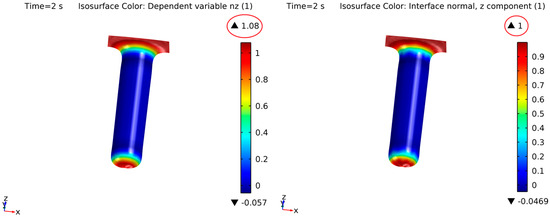
Figure 2.
Normal at the z-direction in a coefficient PDE module with quadratic Lagrangian elements (left). Normal at the z-direction as a direct derivation of the level-set function (right). Maximum punctual normal values are shown in the red circle.
While some precision is lost due to the multiple quadratic discretizations, the gain in simulation speed is noticeable and the problem is now solvable. A summary of the algorithm solving order is provided in Figure 3. The separation in subsystems also helps in the identification of errors, as each derivation step can be easily inspected after the calculation of the solution.
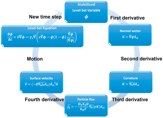
Figure 3.
Summarized scheme of the algorithm computation order.
2.3.2. Solution of Surface Phenomena within a Volumetric Method
As mentioned before, surface diffusion equations, curvature, and surface normal vectors are only valid at the interface or surface of the solid silicon. However, the level-set method is calculated based on the overall simulation domain. If the volumetric divergence/gradient is used and the values at the surface layer (ϕ = 0.5) are inspected, the solution at those points is correct. On the other hand, in other areas outside the interface, the results cannot be controlled. To evaluate this, a reference cylindrical trench was used. Figure 4 shows this trench with the surface in green and a cross-section plane, where the surface with an arbitrary thickness (the co-called concentrating interface function) is shown in red. From this example, calculations of the z and y components of the normal vector are shown in Figure 5 and Figure 6, respectively. On the right side, the solution only at the interface can be observed, giving a correct solution. However, the overall domain solution is displayed on the left side. It can be seen that the values of the normal vectors oscillate in the bulk of the material, especially at the boundaries of the system. When these values are spatially differentiated, the results in the bulk will be suboptimal, affecting the simulation results due to oscillations in the solution and unrealistically large values after the derivation. This affects the convergence of the solution, as the method tolerance must be fulfilled in the overall simulation domain. In addition, such effects in the bulk can spontaneously generate new phases due to incorrect solution regions and thus a reduction in the impact of the surface solution on the bulk, as well as the opposite, becomes necessary.
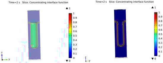
Figure 4.
Cylindrical geometry (green surface) and concentrating interface function (red in the cross-sectional plane) (left). Concentrating interface function is shown in red (right).
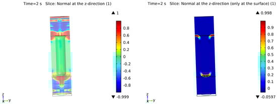
Figure 5.
Normal calculation in the z-direction: with the standard calculation (left) and after applying the values just at the surface interface (right).
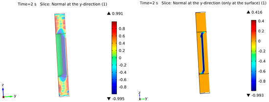
Figure 6.
Normal calculation in the y-direction: with the standard calculation (left) and after applying the values just at the surface interface (right).
For that purpose, two approaches are used simultaneously:
- Define the surface gradient and divergence, i.e., solve the equations along the direction parallel to the surface (where the solution actually exists);
- Define a so-called “interface concentration function”, whose purpose is to decrease the effects of the numerical errors in the bulk, while avoiding a significant reduction of the solution obtained at the interface.
The first part of the proposed method consists in adding a surface divergence, or gradient, to the volumetric domain. For that, it is necessary to split the divergence/gradient in the normal and parallel direction. The definition of the normal divergence is [52,54,55]:
The surface divergence/gradient is then the difference of the total divergence/gradient minus the portion in the normal direction:
or, in tensorial form [52,54,55,56,57], where I is the identity tensor:
Equation (21) can only be used with very precise values of the normal, i.e., with exact values from zero to one. It was discussed in Section 2.3.1 that the approach with the quadratic Lagrangian elements gives only approximate solutions of the normal, which is not a sufficient condition for using Equation (21). To avoid that, COMSOL Multiphysics® includes a function that allows a very accurate determination of the normal vector at the interface within the level-set method. These normal vectors are invoked by the functions “ls.intnormx”, “ls.intnormy”, and “ls.intnormz” for the normal in x, y, and z directions, respectively. These functions are based on Equation (15) after applying a polynomial preserving recovery [41,58,59,60], a post-processing technique that allows a better numerical gradient reconstruction of the mesh elements. However, as explained in Section 2.3.1, when those functions are discretized and coupled with the rest of the equations, the simulation times increase exponentially and the convergence is difficult to achieve. Furthermore, the non-linearity of the equations increases with the surface formulation of the gradient/divergence. A feasible computational solution is to treat the accurate normal vectors as constants to prevent its contribution to the Jacobian of the system. This would have a low impact on the solution, as the accurate normal vectors are only used to accept or discard some part of the divergence/gradient depending on the direction of the surface. This is performed in COMSOL Multiphysics® by using the function “nojac”, which is effectively equivalent to taking the normal values of the previous time step of the simulation (now with subscript “t−1”). This is an acceptable solution if the difference between time steps is small. This developed approach provides acceptable simulation times.
Simplifications of Equation (21) have been frequently used for surface tension phenomena in computational fluid mechanics for a single derivation step [23,56,61]. However, this is not sufficient for the surface diffusion formulation, which needs another additional tweak. The surface operations described above can produce overshoots and undershoots after the derivation next to the surface area or in the bulk phase. For instance, the curvature from the geometry of Figure 4 is shown in more detail in Figure 7 with the surface divergence approach. The left side shows the computed solution, with the maximum curvature in the bulk gas phase and domain boundaries, which is frequently the source of singular points and further unrealistic evolutions in the simulation. At the right side, the curvature is correctly shown after multiplying an approximation of a discrete Kronecker delta function, δK, centered at the interface (ϕ = 0.5):
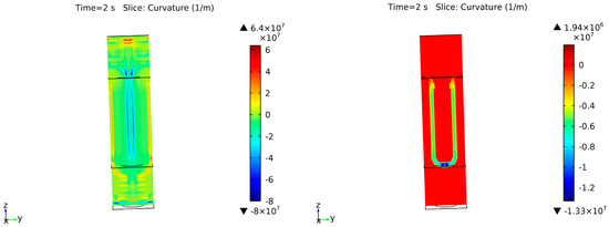
Figure 7.
Curvature calculation in the overall geometry from Figure 4 with the surface divergence approach (left) and the same example after applying the values just at the surface interface (right).
This is the second addition needed to the proposed equations. It consists of the implementation of a multiplying concentrating interface function [57,62], similar to the delta of Kronecker. Unfortunately, the simulation uses continuous Lagrange functions and thus needs a continuous approximation of the function in Equation (22). To ensure the compatibility with the level-set method, and after thorough testing of different approaches, the following concentrating interface function, δci, developing on Equation (14), is selected:
With this approach, the function itself does not introduce any numerical instabilities and is fully compatible with the level-set method while scaling proportionally to the mesh size of the geometry. The concentrating interface function is multiplied after every derivation step to reduce the effect of residual values in the bulk phase, which may be larger than the value at the surface otherwise, even when surface derivatives are used. Furthermore, before introducing the surface velocity field in the level-set method, an ith power of the delta function is used to further reduce the effect of such bulk phases. This tunable parameter may be fitted according to the simulation geometry and mesh. A general working and recommended value is i = 4.
Finally, the final equations can be set, taking into consideration all the changes and effects already described. In the following, the subindices “x, y, z” correspond to the Cartesian axes, while the superindex “t − 1” is the value from the previous time step (invoked by the function “nojac” in COMSOL Multiphysics®). All equations are computed with quadratic Lagrange elements.
The first function, after an initialization step of the level-set variable, is the normal vector:
The next step is to calculate the curvature:
With the curvature, the surface atomic flux is calculated with Equation (7):
The normal velocity of the surface, Equation (8), is then
and the velocity vector can readily be calculated with the normal velocity and the normal vector:
The velocity is then used in the stabilized level-set method:
It should be noted that using the concentrating interface function without considering the surface divergence/gradient produces incorrect results: when δci increases in the direction perpendicular to the interface, the spatial derivative in this direction gives increased curvature values with opposite signs when approaching the interface from either side of it. This is due to the dominant influence of the concentrating interface function, as shown in Figure 8 (right), where the curvature values of the surface displayed in Figure 8 (left) cancel each other out. The second possible issue is an oscillating solution, in which the curvature oscillates on the plane of the surface when the curvature must be constant, as shown in the half-cylinder surface of Figure 9. Thus, it is crucial to use the surface divergence/gradient along the concentrating interface function.
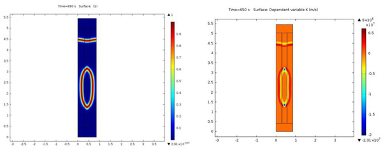
Figure 8.
Curvature calculation (right) when the concentrating interface function, showing the surface position (left), is used with no surface divergence.
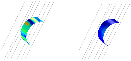
Figure 9.
Curvature calculation of half-cylinder section when the volumetric divergence is used, resulting in a wrong solution (left) and a curvature solution with a surface divergence formulation (right).
The set of equations that ranges from Equations (24) to (29) summarizes the custom level-set method for surface diffusion that is employed in the Section 3. Further parametrizations and boundary conditions are described in the following subsection.
2.3.3. Boundary Conditions and Parametrization of the Simulation
The first modelling step is to define the simulated geometry. As the model must be validated with experimental literature data, the most frequent geometries must be reproduced, even when the presented approach is not geometry-dependent. The objective of this work is centered on the non-coalescence case of cylindrical [12,13,15,63,64,65,66,67,68,69] and rectangular [11,12,13] initial trenches, which are the most frequently investigated cases. In most cases, several trenches are etched in a rectangular matrix that looks similar to the top-view distribution shown in Figure 10. In experiments, this distribution is used to check the limits of the coalescence of different aspect ratios at different trench distances. From the simulation perspective, simulation times can be significantly reduced with such a trench distribution due to the presence of multiple symmetry planes, which serves as a distinct advantage. Consequently, only the colored areas of Figure 10 were simulated in the model, taking the symmetry planes as the lateral boundaries of the model.
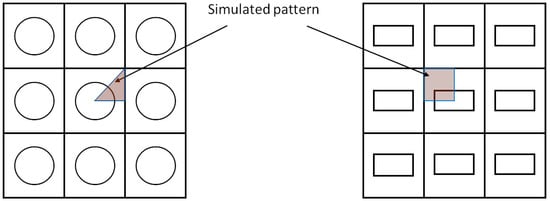
Figure 10.
Section simulated of the pattern as seen from the top for cylindrical trenches (left) and rectangular trenches (right).
Details of the simulated circular sector of the mentioned cylindrical trenches and the overall geometry obtained after applying the symmetries are shown in Figure 11 and Figure 12. In the case of the rectangular trench, the simulated pattern and the view after using symmetry are displayed in Figure 13 and Figure 14, respectively. The boundary planes of the cylindrical and rectangular case (top, bottom, and sides) are shown in Figure 11 and Figure 13, respectively.
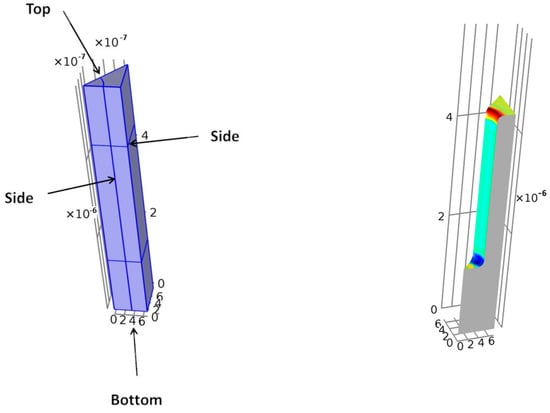
Figure 11.
Simulated circular sector: initial sector definition (left) and initial simulated geometry (right). Color changes with the curvature value.
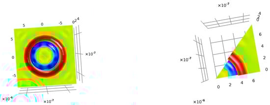
Figure 12.
Simulated cylindrical trench from the top view: initial simulated sector (right) and geometry after applying the corresponding symmetries (left). Color changes with the curvature value.
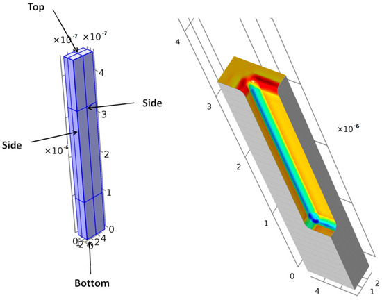
Figure 13.
Simulated rectangular sector: initial sector definition (left) and initial simulated geometry (right). Color changes with the curvature value.
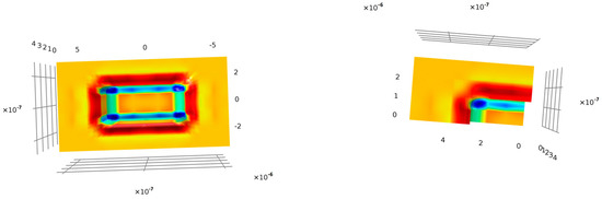
Figure 14.
Simulated rectangular trench from the top view: initial simulated sector (right) and geometry after applying the corresponding symmetries (left). Color changes with the curvature value.
Regarding the boundary conditions, a constant bulk phase at the upper and bottom boundaries must be forced; thus, there will be no normal, curvature, atomic flux, or normal velocity. This prevents the formation of new phases at those boundaries. The distance of the top and bottom boundaries with respect to the surface where the phenomena are taking place should be sufficiently large to avoid any interaction between them. The sufficient boundary condition on the sides is symmetrical, i.e., the derivative of any potential field in the direction of the boundary plane and the vector values projected to the normal of the boundary surface must be zero at that boundary. The corresponding boundary conditions and the description of their effects are summarized in Table 1.

Table 1.
Boundary conditions used for the surface diffusion calculation with the presented custom level-set method.
Concerning the stability factors of the level-set Equation (29), interface thickness ε and the reinitialization parameter γr, they must be properly chosen to ensure the stability of the equation without greatly affecting the real equation solution. The interface thickness is chosen to be half the maximum element size, which is a typical standard value to fulfill the Péclet number Equation (13). As mentioned before, the reinitialization parameter frequently takes a fixed value for the overall simulation. This typically corresponds to the maximum velocity expected during the whole simulation process to fulfill again the Péclet number Equation (13). Nevertheless, during the surface diffusion process, the velocity of the surface is very variable. In the beginning, the velocity of the surface undergoing surface diffusion tends to be significantly high, while the transformation is very slow when reaching the final equilibrium geometries. Thus, a fixed value usually underestimates or overestimates the effect of the stabilization diffusion. As a consequence, if γr is underestimated, the interface may break and instabilities may appear. On the other hand, if it is overestimated, an artificial diffusion from the stabilization part may dominate and create a new non-real diffusion path. The approach of this work is to have a γr value that is updated in every time step to adapt it to the velocity changes; more precisely, the reinitialization parameter will take the module of the maximum velocity value in the system at every time step. This increases the simulation time but, with this approach, a much better stability is achieved. Furthermore, due to the defined concentrated interface function, δci, the values of the velocity are directly from the surface, reducing the possibility of utilizing unrealistic peak velocity values from the bulk that may have arisen from numerical artifacts. As a summary, the stability factors, taking into consideration that h is the mesh size, are then
Regarding the mesh size, it influences the simulation behavior. Coarser meshes can lead to rapid unrealistic movement of the surface or unexpected coalescence processes before the surface can touch the boundary. On the other hand, very fine meshes tend to show a very slow process and an almost impossible coalescence while provoking the appearance of spontaneous new void volumes in any part of the geometry, especially next to the boundaries. After some testing, the working mesh sizes that showed a proper solution were quite limited and corresponded to uniform meshes in all directions. Therefore, relatively constant hexahedral elements were selected due to their capacity for a more regular form in all directions while keeping more information of the derivation in all mesh element directions when compared to more simple tetrahedral elements [41,43]. Such meshes can be observed in Figure 15.
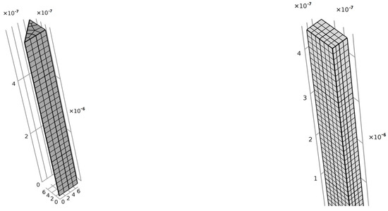
Figure 15.
Typical mesh size and distribution for circular sectors (left) and rectangular sectors (right).
Due to the decoupling of the equations, every derivation step can be explored to check the consistency of the results, which is an advantage of the developed model. For instance, in Figure 16, for the rectangular case, the curvature values (left side) at the surface, the normal velocity of the surface (right), and the atomic current density (right, in form of arrows) are shown, demonstrating that the velocity of the interface is consistent with the atomic migration direction. Analogously, in Figure 17, the result of the four main PDEs are displayed at the surface level (ϕ = 0.5): normal vector (z-axis), curvature, surface atomic flux (z-axis), and normal velocity. Naturally, as the derivation order increases, the precision in the calculation is reduced and, thus, the normal velocity distribution is not as smooth as the other calculated variables. However, the results are consistent with the expectations, they have the corresponding expected orders of magnitude, and the simulation is now feasible for any kind of initial geometries and for any kind of trenches.
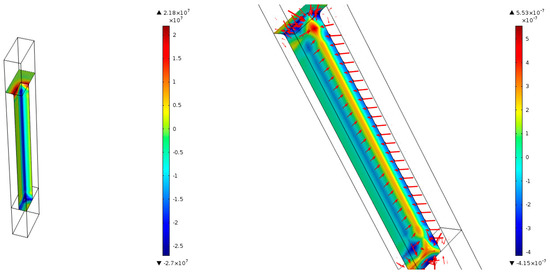
Figure 16.
Curvature of a rectangular trench at the surface level (left) and a combination of the normal velocity represented by the color scheme and the direction of the atomic current density represented by the red arrows (right).
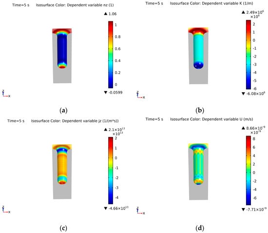
Figure 17.
Result on the solid surface of (a) the z-component of the normal vector, (b) the curvature, (c) the z-component of the atomic current density, and (d) the normal velocity of the surface.
Concerning the solver, a direct solver was used due to its higher robustness and the need for less solver optimization to obtain a result. In this regard, the built-in COMSOL Multiphysics® solvers were employed in the simulations. Both available direct solvers, MUMPS or PARDISO, can solve the proposed model, and both give comparable results. Choosing one over another depends on the number of cores and available memory as one of them may be faster. In the tested systems, the overall simulation times were also similar. Another feature that must be tuned for the simulation is the so-called “variable scale”. This is used during the solving process of the Jacobian, where the solved variables are adimensionalized by dividing the solving variable by the mentioned variable scale. As a consequence, this must be tuned for every simulation. In order to perform such optimization, a small simulation with a few initial time steps is suggested. From that result, the maximum absolute values of the normal, curvature, atomic current density, and normal velocity are used as the corresponding variable scale. When the order of magnitude of the variable scale and the solution of those variables match, it is easier to reach the convergence. Furthermore, a relative tolerance of 10−12 is used to ensure the simulation solution is sufficiently precise, preventing large time steps that would lead to skipping certain stages of the geometrical evolution. This approach guarantees that the geometry of the two most recent time steps remains largely consistent, thereby preserving the validity of the simplification employed in calculating the surface divergence/gradient.
Finally, Table 2 shows the assumed values of the material parameters of the simulation. The activation volume is calculated solely from the data of [29]. Silicon surface free energy density and atomic density are based on the crystal orientation (100), which is the most common tested silicon crystal orientation. Furthermore, an isotropic approach is assumed. In this work, the focus is on the geometrical evolution of the void structures. Thus, the annealing times of the simulation, which depend on the given material parameters, are provided for reference. However, the model was not fitted or thoroughly investigated to match experimental annealing times. Nonetheless, it is a good starting point to see how such a standard formulation deviates from the different experimental results.
Table 2.
Material parameters used in the custom level-set simulation for surface diffusion.
The details of the developed custom level-set method for surface diffusion and the parameters of the simulation are now complete. The results are shown and discussed in the next section.
3. Results and Discussion
In this section, qualitative and quantitative model results are compared to experimental data in the literature, along with simulation data from previously proposed models: moving mesh method model [22] and the published quick analytical model [26]. The results are evaluated and discussed to assess the goodness of the model and the possible limitations.
3.1. Qualitative Model Evaluation
Qualitative results should show if the model is working as intended. For this, a reference cylindrical geometry was tested with typical processing conditions. The qualitative results are shown in Figure 18:
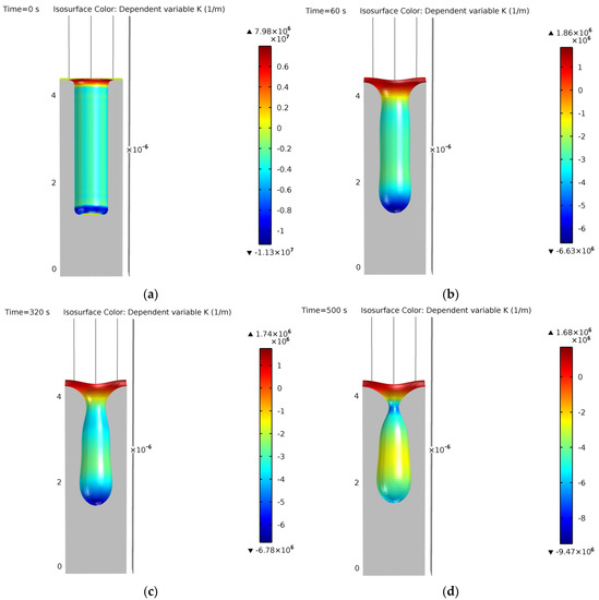
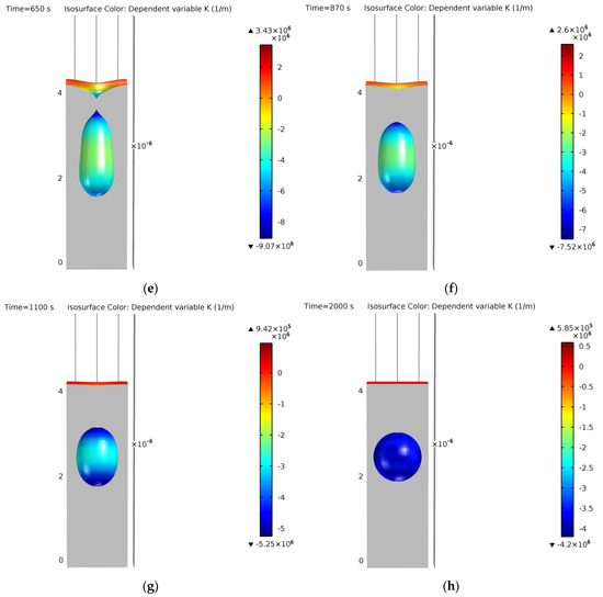
Figure 18.
Typical simulation of a cylindrical trench without coalescence at (a) 0 s, (b) 60 s, (c) 320 s, (d) 500 s, (e) 650 s, (f) 870 s, (g) 1100 s, (h) 2000 s. Colors show curvature values.
- The initial cylindrical trench is shown at t = 0 s in Figure 18a;
- There is a surface free energy minimization process. This can be observed by the rounding of the geometry at the bottom during the first simulation steps. At the same time, a rounding of the top starts to narrow down, getting closer to a “pinch-off” of the void structure that would isolate the internal void from the external atmosphere. This can be observed from Figure 18b (t = 60 s) to Figure 18d (t = 500 s);
- Finally, the internal ESS is closed, a first ellipsoidal void is formed, and it evolves by surface minimization to a perfect equilibrium sphere (constant curvature). On the top surface, the interface smooths out until achieving a planar equilibrium surface (also constant curvature) and finishing the void evolution process. This can be observed from Figure 18e (t = 650 s) to Figure 18h (t = 2000 s).
The model can qualitatively represent the expected void shape evolution of silicon [1,11,12,13,14,15,63]. However, until the model is validated against experimental literature results, which is performed in Section 3.2, a complete validation of the model cannot be completed.
Additionally, another qualitative comparison was performed: the same reference structure was used to study the volume preservation of the model. Theoretically, the surface diffusion equation should ensure the volume conservation. However, the formulation of the custom level-set method had different approximations that are expected to have an influence on this. The question here is the magnitude of the deviations and if the model can, at least, identify the equilibrium geometries. The result of the tracking of the solid volume is given in Figure 19.
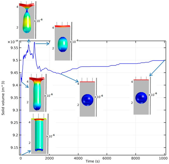
Figure 19.
Volume of the solid part of the body with the simulated time. Geometries at different positions are shown with the arrows. Colors are dependent on the curvature values.
Figure 19 shows that there is a volume change, especially when there is a steeper geometrical transformation. However, when reaching the final equilibrium geometry, the volume stays relatively constant, which is a desired feature of the model. If the model does not cause the final geometry to significantly grow or shrink, it means that the numerical inaccuracies of the proposed model are not so high, allowing the evaluation of final structures when such a solid volume is almost constant. One of the aims of this model was to keep the volume within a 10% range, which is a variation that can already be seen in the experimental data when the structures are etched. In general, in the studied literature values, there are often discrepancies between the objective etched geometries values and the values measured through scanning electron microscope. This is due to the difficulty of etching nano-/microstructures. Consequently, a 10% change in volume can be considered a reasonable margin of error. In fact, the reference case, see Figure 19, had only about a 5% peak-to-peak volume variation. It is crucial to note that, during the testing of different modelling alternatives, other level-set approaches could not maintain the final spherical form without the presented model modifications.
In this context, in COMSOL Multiphysics®, a so-called “volume preservation” level-set method can be employed, which modifies the advection part of the level-set equation. However, the different tests performed with that modification could only help in volumetric phenomena (CFD and similar). The combination of such modification with surface diffusion formulation would just generate non-existent phases in the middle of the geometry when it was able to converge. For this reason, this option was discarded.
Both qualitative tests are within the expectations and verify the capabilities of the model. Regarding the simulation times, depending on the geometry and the number of mesh elements used, a single geometry can take between one/two days and one/two weeks of simulation time. The computation of the model does not scale well beyond the use of 4–6 cpu cores.
The qualitative model evaluation is now complete and the quantitative one is shown in the next subsection.
3.2. Quantitative Model Evaluation
In this subsection, a comparison of the model against quantitative data from the literature is performed. The comparison is divided into cylindrical and rectangular trenches. At the same time, there is a separation between the different output options: final equilibrium geometries (final spherical void) and intermediate geometries that were obtained with lower processing times. The selected model geometries are chosen with a similar evolution stage of the experimental values in the literature. Table 3 summarizes the geometrical parameters used for the comparison. A further visual clarification is found in the void transformation from an initial cylindrical trench shown in Figure 20. For rectangular trenches, the nomenclature is the same, except for the cylindrical radius, which is replaced by the two sides, l1 and l2, of the rectangular base.
Table 3.
Nomenclature and description of the compared features in the Section 3.
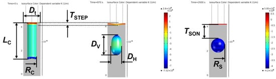
Figure 20.
Geometrical features of a cylindrical trench transformation from initial to final void evolution.
In the following subsections, the equilibrium and intermediate geometries are compared. The values obtained from literature data with the symbol “~” are estimated from SEM figures or diagrams and the accuracy may be reduced. The rest of the literature values are given directly by the corresponding publication. The values “-“ are values that are not found, cannot be calculated, or have small relevancy. The structure of the quantitative evaluation is as follows: first, a data table of the initial geometries is introduced; the second step is to show some of the most relevant simulation results; finally, all data are compared and discussed. The first test case is the spherical equilibrium geometry.
3.2.1. Simulation of Final Equilibrium Voids
The gathered literature results of this subsection are all from rectangular trenches. Their initial geometrical features are summarized in Table 4. The literature data is already scarce, and it is usually subdivided into very specific cases, making the data availability complicated. Nonetheless, 12 different simulations were performed for comparison. However, the distance between trenches was mostly not given in the literature. Therefore, it was assumed to be two times the side of the initial trench.
Table 4.
Tested initial literature values that created a spherical equilibrium void from initial rectangular trenches.
The most interesting and characteristic simulation results of this subsection are now briefly discussed. The first unique case corresponds to example 1, which is the only one that presents no spherical void, but just a planar surface at the end of the evolution. The simulation of the structure evolution from a rectangular trench to an equilibrium planar surface is shown in Figure 21. In Figure 21b, the void evolution would follow the usual known pattern. However, the aspect ratio is too small so a “pinch-off” of the void is not achieved. From Figure 21c on, the internal void smooths out and disappears, leaving only a final planar surface as expected from [11,13].
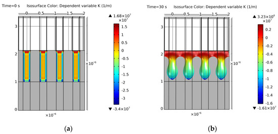
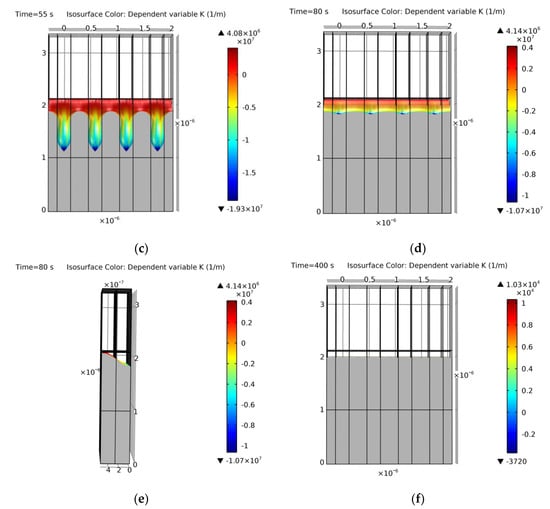
Figure 21.
Simulation of example 1. Cross-section of the results at the following simulation annealing times: (a) 0 s (initial geometry); (b) 30 s; (c) 55 s; (d) 80 s from the front view; (e) 80 s from the side view; (f) 400 s (final equilibrium geometry). Colors show curvature values. The results match [11,13].
A more common result is shown in Figure 22, where the initial rectangular trench of example 2 transforms to an equilibrium sphere. This type of transformation is found from example 2 to example 10. The results from example 3 to example 10 can be found in Appendix A (Figure A1 for examples 3 and 4, Figure A2 for examples 5 and 6, Figure A3 for examples 7 and 8, Figure A4 for examples 9 and 10), yielding similar results to the compared literature values [13]. A complete evolution of example 8 can also be found in Video S1.
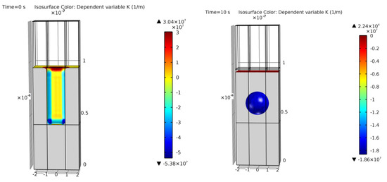
Figure 22.
Simulation of example 2. Cross-section of the initial geometry with a base trench of 0.17 μm × 0.17 μm at t = 0 s (left) and final equilibrium geometry at t = 10 s (right). Colors show curvature values. Void geometrical result within a 9% error of [13].
A corner case is found in Figure 23 with examples 11 and 12. The initial rectangular trench transforms into two spherical voids instead of one in literature [13]. It is difficult to assess why this occurs, as it may be due to differences in the given literature data, the assumed distance between trenches, or the model. As shown in Table 4, these are the initial structures with the highest possible aspect ratio (depth/radius relation). It may be at the boundary where small deviations could form more than one empty space in silicon [26]. On the other hand, with examples 11 and 12, it is demonstrated that the model can also potentially represent cases where more than one ESS is created.
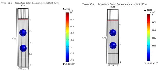
Figure 23.
Cross-section of the final simulation results of examples 11 (left) and 12 (right). Colors show curvature values. Two ESSs generated instead of one in [13].
All the model results along the absolute and relative errors are shown in Table 5. Figure 24 shows the graphical difference between the experimental data, the custom level set model developed in this work, and a previous analytical approach [26] for quick size estimation of equilibrium geometries.
Table 5.
Results of all tested initial literature values that created a spherical equilibrium void. “LS Model” is the developed model in this work.
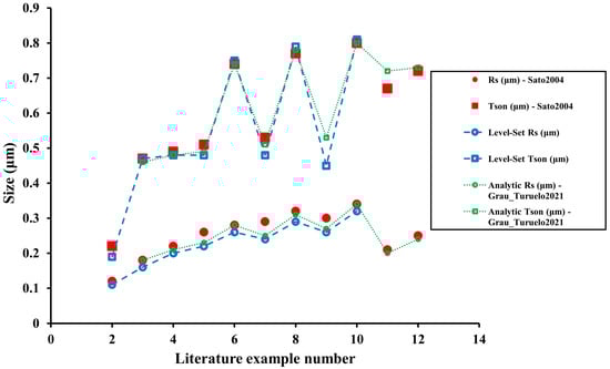
Figure 24.
Summary of the results obtained for final equilibrium geometries. Data (red, Sato2004 [13]) of Table 5 are compared to the custom level-set method of this work (blue) and the analytical model (green) developed in Grau_Turuelo2021 [26]. Same geometrical feature uses the same marker.
As seen in Figure 24, both tested models give very similar results. Both follow the trend of the experimental literature results and can complement each other if one of them does not reproduce the expected geometry. However, the analytical method is frequently slightly more precise in predicting equilibrium geometries than the introduced level-set method. The average calculated relative errors for the developed level-set method are 3.8% and 10.3% for the SON thickness and spherical radius, respectively. Thus, the geometrical solution is relatively accurate, especially considering that the average absolute error of the spherical radius is lower than 0.02 μm, very close to the last significant figure that could be obtained from literature data.
3.2.2. Simulation of Intermediate Voids
Analogous to the previous subsection, the gathered initial geometries of the literature and their respective annealing conditions that would generate an intermediate void are summarized in Table 6 and Table 7. For this second verification process, eight results were found. In the following, the most characteristic model results are shown.
Table 6.
Tested initial literature values that created an intermediate void from initial rectangular trenches.
Table 7.
Tested initial literature values that created an intermediate void from initial cylindrical trenches.
The first displayed simulation is the only rectangular trench of the mentioned tables, example 13, which can be seen in Figure 25. A higher void volume can be observed in comparison to the geometries of Section 3.2.1. This increase in size affects the velocity of the void shape evolution. At the same annealing conditions, a higher geometrical size takes more time for a full equilibrium transformation, preventing the void geometry to completely achieve the perfect spherical void in this case. From Figure 25, it can be observed that the intermediate geometry is not far from the equilibrium one, as expected from [13].
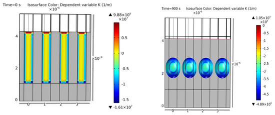
Figure 25.
Simulation of example 13. Cross-section of the initial geometry at t = 0 s (left) and final geometry at t = 900 s (right). Colors show curvature values. Void geometrical result within a 2% error of [13].
Figure 26 shows a typical cylindrical trench simulation from example 14. In this case, there is a relatively high separation of the trenches, and a coalescence is difficult to achieve. The simulation output shows the typical ellipsoid form of the void in silicon when an intermediate step is inspected, yielding similar results to [15,65].
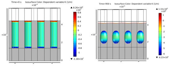
Figure 26.
Simulation of example 14. Cross-section of the initial geometry at t = 0 s (left) and final geometry at t = 950 s (right). Colors show curvature values. Void geometrical result within a 5% error of [15].
Figure 27 was a geometry particularly hard to simulate. The distance between trenches (Figure 27—left) is very small in comparison to the size of the void trench. In nearly every level-set approach, this would generate a coalescence in the beginning that the experimental output does not show. With the proposed model, the separated voids could be maintained longer before merging, allowing the positive evaluation of this particular simulation output [15].
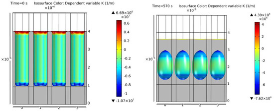
Figure 27.
Simulation of example 16. Cross-section of the initial geometry at t = 0 s (left) and final geometry at t = 570 s (right). Colors show curvature values. Void geometrical result within a 14% error of [15].
Finally, the two special cases (example S.C. and S.C. 2) are shown in Figure 28 and Figure 29, respectively. Due to the very small transformation at the given annealing conditions, the results are very difficult to evaluate quantitatively. For this reason, they are not carried forward. However, the geometry achieved in the simulation is very similar to the one obtained in the literature examples [15]. Figure 29 has the same initial geometry as Figure 27. As mentioned before, even at this early stage of the transformation process, the narrow distance between trenches would produce the coalescence from the beginning with other level-set approaches. However, the proposed model of this work resembles again the expected experimental output [15].
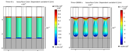
Figure 28.
Simulation of example “S.C.”. Cross-section of the initial geometry at t = 0 s (left) and final geometry at t = 28,000 s (right). Colors show curvature values. Void geometrical results match the geometry expected in [15].
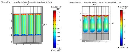
Figure 29.
Simulation of example “S.C. 2”. Cross-section of the initial geometry at t = 0 s (left) and final geometry at t = 20,000 s (right). Colors show curvature values. Void geometrical results match the geometry expected in [15].
The examples not shown here are collected in Appendix B (Figure A5 for example 16 and Figure A6 for examples 17 and 18). Additionally, the evolution of examples 15, 17, and 18 can be found in Video S2 (15) and Video S3 (17 and 18). All the model results corresponding to the intermediate void geometry and the absolute and relative errors of the simulations are summarized in Table 8.
Table 8.
Results of all tested initial literature values that created an intermediate void. “LS Model” is the developed model in this work.
For this kind of final geometry (non-equilibrium), the analytical model of the previous subsection cannot be used. For this reason, a moving mesh method [22] is compared with the level set method for the vertical geometrical features (step, SON layer, and vertical axis of the ellipsoidal void) in Figure 30 and the horizontal geometrical features (horizontal axis of the ellipsoidal void) in Figure 31.
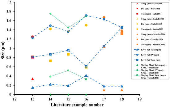
Figure 30.
Summary of the results of the obtained vertical distances for intermediate void geometries. Data (red for Sato2004 [13], yellow for Sudoh2009 [15], orange for Mueller2006 [65]) of Table 8 are compared to the custom level-set method of this work (blue) and a previous moving mesh model (green) developed in Grau_Turuelo2014 [22]. Same geometrical feature uses the same marker.
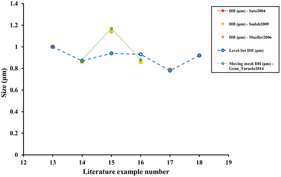
Figure 31.
Summary of the results of the obtained horizontal distances for intermediate void geometries. Data (red for Sato2004 [13], yellow for Sudoh2009 [15], orange for Mueller2006 [65]) of Table 8 are compared to the custom level-set method of this work (blue) and a previous moving mesh model (green) developed in Grau_Turuelo2014 [22]. Same geometrical feature uses the same marker.
As seen from Figure 30 and Figure 31, the level-set method provides a much better accuracy at representing the intermediate void structures than the moving mesh method, especially when evaluating the vertical geometrical features. It is somewhat different for horizontal measurements as the moving mesh was able to outperform the proposed level-set with example 15. Except for that particular example, the trend of the proposed level-set method is very similar to the literature geometries, and even in example 15, the vertical axis of the void ellipsoid and the SON layer are very similar. The most significant outlier in Figure 30 with respect to the level-set method corresponds to the step size of example 13. All geometrical features are almost identical except for the step size. This may be generated by the use of symmetries as the upper part of the geometry may be influenced by the surroundings, something that the symmetric condition (to achieve better simulation times) simplifies. The effect of the symmetry is equivalent to a simulation of infinite trenches that are etched on an infinite surface. In reality, there are side effects if the trench is relatively close to an area where there are no trenches nearby, something that is not considered with the proposed level-set method. For the remaining results, the custom level-set method is comparable to the literature experiments.
Regarding the calculated errors, the average relative errors were 72.0%, 13.8%, 4.7%, and 5.2% for the step size, SON layer, vertical axis, and horizontal axis, respectively. Therefore, the model provides a good prediction for the void itself. The SON layer is within the expected error range with some precise results (about <5% error for examples 16 and 17) but others were quite inaccurate (>30% in example 13). Finally, concerning the step size, the results are particularly deviated, which, as commented, could be produced from the idealized use of symmetries. However, the step size is frequently not very relevant when designing the structure for potential applications.
After analyzing all these data, it can be concluded that the proposed custom level-set model for surface diffusion is a versatile model. It can be used for both equilibrium and intermediate structures. When compared with the moving mesh method in intermediate structures, the level-set model delivers generally much better results while showing a possible limitation in the computation of the geometrical step sizes, possibly due to the symmetric boundary conditions (moving mesh method was also not better in this regard). However, the symmetric approach saves a lot of simulation time by reducing the amount of mesh elements needed for the simulation.
Regarding the equilibrium structures in Section 3.2.1, the results are comparable to those of the analytical model, which were already significantly precise. Thus, the custom level-set provides an overall balanced solution at the expense of calculation time, making it a suitable tool to use in combination with the analytical model. On the other hand, it displaces the moving mesh method as a simulation solution. It is more precise, it does not need a virtual curvature function based on perturbation dynamics, and level-set methods are compatible with any kind of geometries.
Before the conclusions, and while not being a direct objective of this work, there are additional comments about the simulated annealing times in the next subsection.
3.2.3. Annealing Times and the Surface Diffusion Coefficient
In this subsection, some issues about the annealing times found during the development of the model are discussed. In this work, the used material parameters are described in Table 2. They are relatively standard values for silicon (100), which are used in many articles. However, when inspecting the annealing times of Table 8, the real and simulated annealing times, except for example 15 at 60 Torr and 1150 °C, do not fit.
With the current custom level-set formulation for surface diffusion, the void shape evolution (from initial trenches to final equilibrium shapes) do not geometrically change regardless of the material parameters used. The other material parameters only change the process speed or the annealing time required to achieve a certain geometry. There is only one exception, and that is if the model were anisotropic and/or the surface facets were simulated [15,73], which would increase the simulation complexity exponentially, and it is difficult to couple with the level-set method along with the coalescence phenomena.
Recalling the simulated annealing times of Table 8, no systematic error can be observed. Sometimes, the simulation annealing times are higher than the experimental ones; at other times, they are lower. Most of the material parameters (atomic volume, surface atomic density, etc.) are constant (or they would have a relatively low variation) and their impact on annealing speed should be proportional to their values. Therefore, they must not be the source of those inaccuracies. The most likely source is the surface diffusion coefficient. The Arrhenius temperature behavior has already been demonstrated [14,28,70], and thus, the issue relies on the pressure formulation. Almost every experimental void shape evolution in the literature is carried out at different combinations of temperature and pressure. However, pressure data are usually lacking and there is a lack of affecting pressure models available. It was demonstrated that the hydrogen pressure has an influence on the void shape evolution [27,29,70], that the argon pressure [28,64,66,67,74] also has such an influence when using it as annealing gas, and that different gases also affect the transformation speed [74]. Therefore, there are two factors that are often overlooked: type of annealing gas and pressure of such gas. They are necessary if the correct annealing time must be determined. Otherwise, the model material parameters can only be fitted at certain fixed annealing conditions (always-same pressure and same gas). This fact opens up new investigation paths that could lead to better knowledge and controllability of the void shape evolution process in silicon.
The last discussion point of this work is the adaptability of this model to different materials, including different silicon modifications, such as doped silicon. As already discussed, according to the presented surface diffusion model, the used materials do not change the geometrical evolution but the evolution speed. Materials that are known to block the geometrical transformation of the void shape evolution of silicon, such as silicon oxide or silicon nitride [12,66,69], can be regarded in this model as materials that have a very low surface diffusion coefficient. The lower the surface diffusion coefficient, the lower the transformation speed (see Equation (8)); thus, the evolution time tends toward infinity when the surface diffusion coefficient tends toward zero. In order to adapt the model to other materials, four material properties must be readjusted: the surface diffusion coefficient DS, the surface atomic density XS, the surface free energy density γ, and the atomic volume Ω. In the case of a modified silicon structure, such as doped silicon or another surface orientation, the deviation in any of those four properties must be studied and modified in the model parameters (for instance, for Si (111), a modification of the surface energy and surface atomic density should be at least performed). In the case of a heterogeneous composition or doping, the material properties could be averaged for a first modelling approach. Consequently, the presented model can be adapted to a wide range of materials that may present a geometrical transformation due to a surface diffusion phenomenon.
4. Conclusions
This work proposes a newly developed custom level-set model to simulate the evolution of void structures in silicon by surface diffusion phenomena. The considered approach consists of the coupling of the volumetric formulation of the level-set method with the surface formulation of the surface diffusion. In order to accomplish this, the coupling of both equations, which form a non-linear fourth-order PDE, is divided into smaller equations, combining a quadratic discretization order per derivation step with a so-called concentrating interface function, to reduce the numerical instabilities occurring in each bulk phase. In order to reduce the impact of the bulk phase on the surface formulation, a surface divergence/gradient is formulated which transforms the volumetric spatial derivation, needed for the level-set variable, to a surface one.
The described modifications along with the definition of suitable stabilization level-set parameters allows the complete simulation of the non-coalescence case of the void shape evolution in silicon. The level-set method can be used for complete morphological transformations and potentially also for the coalescence of void structures. The volume variation was tested to be around 5% in peak-to-peak values.
The model working conditions were verified with non-coalescence cases found in the literature. The comparisons reflect a highly versatile model that follows the trend of most experimental data and that can simulate intermediate and equilibrium void structures while providing better accuracy than other simulation methods, such as the moving mesh method in the former case, and similar accuracy in comparison to the presented analytical method in the latter case.
The proposed and versatile custom level-set method for surface diffusion has the additional advantage that it can be used for any material undergoing the same phenomena (by changing the material parameters), it can simulate any void geometry, and it can potentially simulate coalescence (there is a small test case in Appendix B, Figure A6). On the other hand, it also has some limitations, such as the lack of complete volume conservation, some small numerical accuracies due to the approximations taken for performing the simulation in feasible computational times (between one or two days and one or two weeks), and the simplification of border effects due to the symmetrical approach.
Finally, the proposed model is a suitable tool to use in combination with the previous developed analytical model [26]. They can work together as a toolbox for the control and prediction of void structures.
Supplementary Materials
The following supporting information can be downloaded at: https://www.mdpi.com/article/10.3390/cryst13060863/s1, Video S1: Evolution of example 8 (Figure A3-right) in 1 s steps until 100 s; 10 s steps from 100 s to the end.; Video S2: Evolution of example 15 (Figure A5) in 1 s steps until 100 s; 10 s steps from 100 s to the end.; Video S3: Evolution of examples 17 and 18 as shown in Figure A6 (different color scheme), evolution in 1 s steps until 100 s; 10 s steps from 100 s until 1000 s; 100 s steps from 1000 s to the end.
Author Contributions
Conceptualization, C.G.T. and C.B.; methodology, C.G.T.; software, C.G.T.; validation, C.G.T.; formal analysis, C.G.T.; investigation, C.G.T.; resources, C.B.; data curation, C.G.T.; writing—original draft preparation, C.G.T.; writing—review and editing, C.G.T. and C.B.; visualization, C.G.T.; supervision, C.B.; project administration, C.B.; funding acquisition, C.B. All authors have read and agreed to the published version of the manuscript.
Funding
Part of this work was funded by the European Social Fund (ESF), the “Sächsische Aufbaubank” (SAB), and the Saxon State Ministry of Science and Art (SMWK) by a Ph.D. “National Innovation Scholarship”, application number: [100119076].
Data Availability Statement
Calculated data, model configuration, model equation, software, and compared sources are given within this manuscript and in Supplementary Materials. Intermediate results or other computed variables of the shown simulations can be made available upon request.
Conflicts of Interest
The authors declare no conflict of interest.
Appendix A
In this appendix, a compilation of all simulated results from Section 3.2.1, Table 5, which are not shown in the main text, can be found. The Figure A1, Figure A2, Figure A3 and Figure A4 are self-described with their own caption.

Figure A1.
Cross-section of the final simulation results of examples 3 (left) and 4 (right). Colors show curvature values. Void geometrical result within a 12% and 10% error of [13].
Figure A1.
Cross-section of the final simulation results of examples 3 (left) and 4 (right). Colors show curvature values. Void geometrical result within a 12% and 10% error of [13].


Figure A2.
Cross-section of the final simulation results of examples 5 (left) and 6 (right). Colors show curvature values. Void geometrical result within a 16% and 8% error of [13].
Figure A2.
Cross-section of the final simulation results of examples 5 (left) and 6 (right). Colors show curvature values. Void geometrical result within a 16% and 8% error of [13].


Figure A3.
Cross-section of the final simulation results of examples 7 (left) and 8 (right). Colors show curvature values. Void geometrical result within a 18% and 10% error of [13]. For the complete evolution, Video S1 can be accessed.
Figure A3.
Cross-section of the final simulation results of examples 7 (left) and 8 (right). Colors show curvature values. Void geometrical result within a 18% and 10% error of [13]. For the complete evolution, Video S1 can be accessed.


Figure A4.
Cross-section of the final simulation results of examples 9 (left) and 10 (right). Colors show curvature values. Void geometrical result within a 14% and 6% error of [13].
Figure A4.
Cross-section of the final simulation results of examples 9 (left) and 10 (right). Colors show curvature values. Void geometrical result within a 14% and 6% error of [13].

Appendix B
Analogous to Appendix A, in this appendix, simulated results that are not shown in the main text of Section 3.2.2, Table 7, are compiled. The Figure A5 and Figure A6 are self-described with their own caption.

Figure A5.
Simulation of example 15. Cross-section of the initial geometry at t = 0 s (left) and final geometry at t = 560 s (right). Colors show curvature values. Void geometrical result within a 18% error of [15]. For the complete evolution, Video S2 can be accessed.
Figure A5.
Simulation of example 15. Cross-section of the initial geometry at t = 0 s (left) and final geometry at t = 560 s (right). Colors show curvature values. Void geometrical result within a 18% error of [15]. For the complete evolution, Video S2 can be accessed.


Figure A6.
Simulation of examples 17 and 18. Cross-section of the simulation results at: (a) 0 s (initial geometry, the same for both); (b) 840 s (result of example 17); (c) 1000 s (result of example 18); (d) 2000 s (final equilibrium void after the coalescence). Colors show curvature values. Void geometrical result within a 2% and 8% error of [65]. For the complete evolution, Video S3 can be accessed.

References
- Sato, M.; Matsuo, I.; Mizushima, Y.; Tsunashima, S.; Takagi, S. Method for Fabricating a Localize SOI in Bulk Silicon Substrate Including Changing First Trenches Formed in the Substrate into Unclosed Empty Space by Applying Heat Treatment. U.S. Patent No. 7,507,634, 24 March 2009. [Google Scholar]
- Jurczak, M.; Skotnicki, T.; Paoli, M.; Tormen, B.; Martins, J.; Regolini, J.L.; Dutartre, D.; Ribot, P.; Lenoble, D.; Pantel, R.; et al. Silicon-on-Nothing (SON)-an Innovative Process for Advanced CMOS. IEEE Trans. Electron Devices 2000, 47, 2179–2187. [Google Scholar] [CrossRef]
- Monfray, S.; Skotnicki, T.; Morand, Y.; Descombes, S.; Paoli, M.; Ribot, P.; Talbot, A.; Dutartre, D.; Leverd, F.; Lefriec, Y.; et al. First 80 Nm SON (Silicon-on-Nothing) MOSFETs with Perfect Morphology and High Electrical Performance. In Proceedings of the Electron Devices Meeting, 2001. IEDM’01. Technical Digest. International, Washington, DC, USA, 2–5 December 2001; IEEE: Piscataway, NJ, USA, 2001; Volume 1, pp. 29.7.1–29.7.4. [Google Scholar] [CrossRef]
- Villani, P.; Favilla, S.; Labate, L.; Novarini, E.; Ponza, A.; Stella, R. Evaluation of Self-Heating Effects on an Innovative SOI Technology (“Venezia” Process). In Proceedings of the Proceedings. ISPSD’05. The 17th International Symposium on Power Semiconductor Devices and ICs, Santa Barbara, CA, USA, 23–26 May 2005; IEEE: Piscataway, NJ, USA, 2005; Volume 1, pp. 63–66. [Google Scholar] [CrossRef]
- Röth, A.; Kautzsch, T.; Vogt, M.; Stegemann, M.; Fröhlich, H.; Breitkopf, C. Investigation of Amorphous Hydrogenated Carbon Layers as Sacrificial Structures for MEMS Applications. In Proceedings of the SENSORS, 2014 IEEE, Valencia, Spain, 2–5 November 2014; IEEE: Piscataway, NJ, USA, 2014; pp. 523–526. [Google Scholar] [CrossRef]
- Durand, C.; Casset, F.; Ancey, P.; Judong, F.; Talbot, A.; Quenouillère, R.; Renaud, D.; Borel, S.; Florin, B.; Buchaillot, L. Silicon on Nothing MEMS Electromechanical Resonator. Microsyst. Technol. 2008, 14, 1027–1033. [Google Scholar] [CrossRef]
- Monfray, S.; Skotnicki, T.; Morand, Y.; Descombes, S.; Coronel, P.; Mazoyer, P.; Harrison, S.; Ribot, P.; Talbot, A.; Dutartre, D.; et al. 50 Nm-Gate All around (GAA)-Silicon on Nothing (SON)-Devices: A Simple Way to Co-Integration of GAA Transistors within Bulk MOSFET Process. In Proceedings of the 2002 Symposium on VLSI Technology. Digest of Technical Papers, Honolulu, HI, USA, 11–13 June 2002; IEEE: Piscataway, NJ, USA, 2002; Volume 1, pp. 108–109. [Google Scholar] [CrossRef]
- Hoellt, L.; Schulze, J.; Eisele, I.; Suligoj, T.; Jovanović, V.; Thompson, P.E. First Sub-30nm Vertical Silicon-on-Nothing MOSFET. Proc. MIPRO 2008, 1, 90–95. [Google Scholar]
- Peng, B.; Yu, T.; Yu, F. A Novel Process of Silicon-on-Nothing MOSFETs with Double Implantation. In Proceedings of the 2007 IEEE International Conference on Integration Technology, Shenzhen, China, 20–24 March 2007; IEEE: Piscataway, NJ, USA, 2007; Volume 1, pp. 237–240. [Google Scholar] [CrossRef]
- Bu, W.; Huang, R.; Li, M.; Tian, Y.; Wang, Y. A Novel Technique of Silicon-on-Nothing MOSFETs Fabrication by Hydrogen and Helium Co-Implantation. In Proceedings of the 7th International Conference on Solid-State and Integrated Circuits Technology, Beijing, China, 18–21 October 2004; IEEE: Piscataway, NJ, USA, 2004; Volume 1, pp. 269–272. [Google Scholar] [CrossRef]
- Mizushima, I.; Sato, T.; Taniguchi, S.; Tsunashima, Y. Empty-Space-in-Silicon Technique for Fabricating a Silicon-on-Nothing Structure. Appl. Phys. Lett. 2000, 77, 3290–3292. [Google Scholar] [CrossRef]
- Sato, T.; Mitsukake, K.; Mizushima, I.; Tsunashima, Y. Micro-Structure Transformation of Silicon: A Newly Developed Transformation Technology for Patterning Silicon Surfaces Using the Surface Migration of Silicon Atoms by Hydrogen Annealing. Jpn. J. Appl. Phys. 2000, 39, 5033–5038. [Google Scholar] [CrossRef]
- Sato, T.; Mizushima, I.; Taniguchi, S.; Takenaka, K.; Shimonishi, S.; Hayashi, H.; Hatano, M.; Sugihara, K.; Tsunashima, Y. Fabrication of Silicon-on-Nothing Structure by Substrate Engineering Using the Empty-Space-in-Silicon Formation Technique. Jpn. J. Appl. Phys. 2004, 43, 12. [Google Scholar] [CrossRef]
- Sudoh, K.; Iwasaki, H.; Kuribayashi, H.; Hiruta, R.; Shimizu, R. Numerical Study on Shape Transformation of Silicon Trenches by High-Temperature Hydrogen Annealing. Jpn. J. Appl. Phys. 2004, 43, 5937. [Google Scholar] [CrossRef]
- Sudoh, K.; Iwasaki, H.; Hiruta, R.; Kuribayashi, H.; Shimizu, R. Void Shape Evolution and Formation of Silicon-on-Nothing Structures during Hydrogen Annealing of Hole Arrays on Si(001). J. Appl. Phys. 2009, 105, 083536. [Google Scholar] [CrossRef]
- Hernández, D.; Trifonov, T.; Garín, M.; Alcubilla, R. “Silicon Millefeuille”: From a Silicon Wafer to Multiple Thin Crystalline Films in a Single Step. Appl. Phys. Lett. 2013, 102, 172102. [Google Scholar] [CrossRef]
- Garín, M.; Jin, C.; Cardador, D.; Trifonov, T.; Alcubilla, R. Controlling Plateau-Rayleigh Instabilities during the Reorganization of Silicon Macropores in the Silicon Millefeuille Process. Sci. Rep. 2017, 7, 7233. [Google Scholar] [CrossRef]
- Castez, M.F.; Albano, E.V. Modeling the Decay of Nanopatterns: A Comparative Study between a Continuum Description and a Discrete Monte Carlo Approach. J. Phys. Chem. C 2007, 111, 4606–4613. [Google Scholar] [CrossRef]
- Castez, M.F. Surface-Diffusion-Driven Decay of Patterns: Beyond the Small Slopes Approximation. J. Phys. Condens. Matter 2010, 22, 345007. [Google Scholar] [CrossRef]
- Castez, M.F. N-Fold Symmetric Two-Dimensional Shapes Evolving by Surface Diffusion. EPL (Europhys. Lett.) 2013, 104, 36003. [Google Scholar] [CrossRef]
- Madrid, M.A.; Salvarezza, R.C.; Castez, M.F. One-Dimensional Gratings Evolving through High-Temperature Annealing: Sine-Generated Solutions. J. Phys. Condens. Matter 2012, 24, 015001. [Google Scholar] [CrossRef]
- Grau Turuelo, C.; Bergmann, B.; Breitkopf, C. Void Shape Evolution of Silicon Simulation: Non-Linear Three-Dimensional Curvature Calculation by First Order Analysis. Univers. J. Comput. Anal. 2014, 2, 27–45. [Google Scholar]
- Shin, S. Computation of the Curvature Field in Numerical Simulation of Multiphase Flow. J. Comput. Phys. 2007, 222, 872–878. [Google Scholar] [CrossRef]
- Engquist, B.; Tornberg, A.-K.; Tsai, R. Discretization of Dirac Delta Functions in Level Set Methods. J. Comput. Phys. 2005, 207, 28–51. [Google Scholar] [CrossRef]
- Yue, P.; Feng, J.J.; Liu, C.; Shen, J. A Diffuse-Interface Method for Simulating Two-Phase Flows of Complex Fluids. J. Fluid Mech. 2004, 515, 293–317. [Google Scholar] [CrossRef]
- Grau Turuelo, C.; Breitkopf, C. Simple Algebraic Expressions for the Prediction and Control of High-Temperature Annealed Structures by Linear Perturbation Analysis. MCA 2021, 26, 43. [Google Scholar] [CrossRef]
- Kuribayashi, H.; Shimizu, R.; Sudoh, K.; Iwasaki, H. Hydrogen Pressure Dependence of Trench Corner Rounding during Hydrogen Annealing. J. Vac. Sci. Technol. A Vac. Surf. Film. 2004, 22, 1406. [Google Scholar] [CrossRef]
- Kuribayashi, H.; Hiruta, R.; Shimizu, R.; Sudoh, K.; Iwasaki, H. Investigation of Shape Transformation of Silicon Trenches during Hydrogen Annealing. Jpn. J. Appl. Phys. 2004, 43, L468. [Google Scholar] [CrossRef]
- Lee, M.-C.M.; Wu, M.C. Thermal Annealing in Hydrogen for 3-D Profile Transformation on Silicon-on-Insulator and Sidewall Roughness Reduction. J. Microelectromechanical. Syst. 2006, 15, 338–343. [Google Scholar] [CrossRef]
- Mullins, W.W. Theory of Thermal Grooving. J. Appl. Phys. 1957, 28, 333. [Google Scholar] [CrossRef]
- Zangwill, A. Physics at Surfaces; Cambridge University Press: Cambridge, UK, 1988; ISBN 978-0-511-62256-4. [Google Scholar]
- Suo, Z. Motions of Microscopic Surfaces in Materials. In Advances in Applied Mechanics; Hutchinson, J.W., Wu, T.Y., Eds.; Elsevier: Amsterdam, The Netherlands, 1997; Volume 33, pp. 193–294. [Google Scholar] [CrossRef]
- Wei, Y.; Zhigang, S. Global View of Microstructural Evolution: Energetics, Kinetics and Dynamical Systems. Acta Mech. Sin. 1996, 12, 144–157. [Google Scholar] [CrossRef]
- Mehrer, H. Diffusion in Solids/Fundamentals, Methods, Materials, Diffusion-Controlled Processes; Springer Science & Business Media: Berlin/Heidelberg, Germany, 2007. [Google Scholar]
- Müller, E.W.; Gomer, R.; Stranski, I.N.; Herring, C. The Use of Classical Macroscopic Concepts in Surface Energy Problems. Struct. Prop. Solid Surf. 1953, 72, 5. [Google Scholar]
- Herring, C. Surface Tension as a Motivation for Sintering. Phys. Powder Metall. 1951, 143–179. [Google Scholar]
- Crank, J. The Mathematics of Diffusion, 2nd ed.; Clarendon Press: Oxford, UK, 1975; ISBN 0-19-853344-6. [Google Scholar]
- Olsson, E.; Kreiss, G. A Conservative Level Set Method for Two Phase Flow. J. Comput. Phys. 2005, 210, 225–246. [Google Scholar] [CrossRef]
- Stöcker, C. Level Set Methods for Higher Order Evolution Laws. Ph.D. Thesis, Forschungszentrum Caesar: Bonn and Technische Universität Dresden, Dresden, Germany, 2008. Available online: https://nbn-resolving.org/urn:nbn:de:bsz:14-ds-1205350171405-81971 (accessed on 30 March 2023).
- Lützen, J. Heaviside’s Operational Calculus and the Attempts to Rigorise It. Arch. Hist. Exact Sci. 1979, 21, 161–200. [Google Scholar] [CrossRef]
- COMSOL Multiphysics Reference Manual, Version 5.1, COMSOL, Inc. Available online: www.comsol.com (accessed on 30 March 2023).
- Zhi-liang, W.; Zhe-wei, Z. An Improved Level-Set Re-Initialization Solver. Appl. Math. Mech.-Engl. Ed. 2004, 25, 1083–1088. [Google Scholar] [CrossRef]
- Zienkiewicz, O.C.; Taylor, R.L.; Nithiarasu, P. The Finite Element Method for Fluid Dynamics; The Finite Element Method; Elsevier Science: Amsterdam, The Netherlands, 2013; ISBN 978-0-08-095137-9. [Google Scholar]
- Courant, R.; Isaacson, E.; Rees, M. On the Solution of Nonlinear Hyperbolic Differential Equations by Finite Differences. Comm. Pure Appl. Math. 1952, 5, 243–255. [Google Scholar] [CrossRef]
- Goldman, R. Curvature Formulas for Implicit Curves and Surfaces. Comput. Aided Geom. Des. 2005, 22, 632–658. [Google Scholar] [CrossRef]
- Raessi, M.; Mostaghimi, J.; Bussmann, M. Advecting Normal Vectors: A New Method for Calculating Interface Normals and Curvatures When Modeling Two-Phase Flows. J. Comput. Phys. 2007, 226, 774–797. [Google Scholar] [CrossRef]
- Barrett, J.W.; Blowey, J.F.; Garcke, H. Finite Element Approximation of a Fourth Order Nonlinear Degenerate Parabolic Equation. Numer. Math. 1998, 80, 525–556. [Google Scholar] [CrossRef]
- Zhornitskaya, L.; Bertozzi, A.L. Positivity-Preserving Numerical Schemes for Lubrication-Type Equations. SIAM J. Numer. Anal. 1999, 37, 523–555. [Google Scholar] [CrossRef]
- Grün, G.; Rumpf, M. Nonnegativity Preserving Convergent Schemes for the Thin Film Equation. Numer. Math. 2000, 87, 113–152. [Google Scholar] [CrossRef]
- GrüN, G.; Rumpf, M. Simulation of Singularities and Instabilities Arising in Thin Film Flow. Eur. J. Appl. Math. 2001, 12, 293–320. [Google Scholar] [CrossRef]
- Greer, J.B.; Bertozzi, A.L.; Sapiro, G. Fourth Order Partial Differential Equations on General Geometries. J. Comput. Phys. 2006, 216, 216–246. [Google Scholar] [CrossRef]
- Bruchon, J.; Pino Munoz, D.; Valdivieso, F.; Drapier, S.; Pacquaut, G. 3D Simulation of the Matter Transport by Surface Diffusion within a Level-Set Context. Rev. Eur. De Mécanique Numérique 2010, 19, 281–292. [Google Scholar] [CrossRef]
- Waring, E. VII. Problems Concerning Interpolations. Philos. Trans. R. Soc. Lond. 1779, 69, 59–67. [Google Scholar] [CrossRef]
- Brackbill, J.U.; Kothe, D.B.; Zemach, C. A Continuum Method for Modeling Surface Tension. J. Comput. Phys. 1992, 100, 335–354. [Google Scholar] [CrossRef]
- Tasdizen, T.; Whitaker, R.; Burchard, P.; Osher, S. Geometric Surface Processing via Normal Maps. ACM Trans. Graph. (TOG) 2003, 22, 1012–1033. [Google Scholar] [CrossRef]
- Lafaurie, B.; Nardone, C.; Scardovelli, R.; Zaleski, S.; Zanetti, G. Modelling Merging and Fragmentation in Multiphase Flows with SURFER. J. Comput. Phys. 1994, 113, 134–147. [Google Scholar] [CrossRef]
- Burger, M.; Haußer, F.; Stöcker, C.; Voigt, A. A Level Set Approach to Anisotropic Flows with Curvature Regularization. J. Comput. Phys. 2007, 225, 183–205. [Google Scholar] [CrossRef]
- Guo, H.; Zhang, Z.; Zhao, R.; Zou, Q. Polynomial Preserving Recovery on Boundary. J. Comput. Appl. Math. 2016, 307, 119–133. [Google Scholar] [CrossRef]
- Naga, A.; Zhang, Z. A Posteriori Error Estimates Based on the Polynomial Preserving Recovery. SIAM J. Numer. Anal. 2004, 42, 1780–1800. [Google Scholar] [CrossRef]
- Zhang, Z.; Naga, A. A New Finite Element Gradient Recovery Method: Superconvergence Property. SIAM J. Sci. Comput. 2005, 26, 1192–1213. [Google Scholar] [CrossRef]
- Boufercha, N.; Sägebarth, J.; Sandmaier, H. Simulation of the Dynamic Behaviour of a Droplet on a Structured Surface Using the Non-Conservative Level Set Method. In Proceedings of the European COMSOL Conference, Hannover, Germany, 4–6 November 2008. [Google Scholar]
- Smereka, P. The Numerical Approximation of a Delta Function with Application to Level Set Methods. J. Comput. Phys. 2006, 211, 77–90. [Google Scholar] [CrossRef]
- Sato, T.; Aoki, N.; Mizushima, I.; Tsunashima, Y. A New Substrate Engineering for the Formation of Empty Space in Silicon (ESS) Induced by Silicon Surface Migration. In Proceedings of the International Electron Devices Meeting 1999. Technical Digest. International, Washington, DC, USA, 5–8 December 1999; IEEE: Piscataway, NJ, USA, 1999; pp. 517–520. [Google Scholar] [CrossRef]
- Depauw, V.; Gordon, I.; Beaucarne, G.; Poortmans, J.; Mertens, R.; Celis, J.-P. Large-Area Monocrystalline Silicon Thin Films by Annealing of Macroporous Arrays: Understanding and Tackling Defects in the Material. J. Appl. Phys. 2009, 106, 033516. [Google Scholar] [CrossRef]
- Mueller, T.; Dantz, D.; von Ammon, W.; Virbulis, J.; Bethers, U. Modeling of Morphological Changes by Surface Diffusion in Silicon Trenches. ECS Trans. 2006, 2, 363–374. [Google Scholar] [CrossRef]
- Depauw, V.; Richard, O.; Bender, H.; Gordon, I.; Beaucarne, G.; Poortmans, J.; Mertens, R.; Celis, J.-P. Study of Pore Reorganisation during Annealing of Macroporous Silicon Structures for Solar Cell Application. Thin Solid Film. 2008, 516, 6934–6938. [Google Scholar] [CrossRef]
- Zeng, F.; Luo, Y.; Yobas, L.; Wong, M. Self-Formed Cylindrical Microcapillaries through Surface Migration of Silicon and Their Application to Single-Cell Analysis. J. Micromech. Microeng. 2013, 23, 055001. [Google Scholar] [CrossRef]
- Sudoh, K.; Nakamura, J.; Naito, M.; Higuchi, K.; Maenaka, K. Formation of Silicon-on-Nothing Structures with Extremely Flat Surfaces. Jpn. J. Appl. Phys. 2013, 52, 075601. [Google Scholar] [CrossRef]
- Bopp, M.; Coronel, P.; Judong, F.; Jouannic, K.; Talbot, A.; Ristoiu, D.; Pribat, C.; Bardos, N.; Pico, F.; Samson, M.P.; et al. 3D Nanostructured Silicon Relying on Hard Mask Engineering for High Temperature Annealing (HME-HTA) Processes for Electronic Devices. In Proceedings of the 2008 NSTI Nanotechnology Conference and Trade Show, Boston, MA, USA, 1 June 2008; pp. 634–637, ISBN 978-1-4200-8503-7. [Google Scholar]
- Keeffe, M.E.; Umbach, C.C.; Blakely, J.M. Surface Self-Diffusion on Si from the Evolution of Periodic Atomic Step Arrays. J. Phys. Chem. Solids 1994, 55, 965–973. [Google Scholar] [CrossRef]
- Yaws, C.; Dickens, L.; Lutwack, R.; Hsu, G. Semiconductor industry silicon: Physical and thermodynamic properties. Solid State Technol. 1981, 24, 87–92. [Google Scholar]
- Eaglesham, D.J.; White, A.E.; Feldman, L.C.; Moriya, N.; Jacobson, D.C. Equilibrium Shape of Si. Phys. Rev. Lett. 1993, 70, 1643. [Google Scholar] [CrossRef]
- Kitayama, M.; Narushima, T.; Carter, W.C.; Cannon, R.M.; Glaeser, A.M. The Wulff Shape of Alumina: I, Modeling the Kinetics of Morphological Evolution. J. Am. Ceram. Soc. 2000, 83, 2531–2561. [Google Scholar] [CrossRef]
- Kant, R.; Ferralis, N.; Provine, J.; Maboudian, R.; Howe, R.T. Experimental Investigation of Silicon Surface Migration in Low Pressure Nonreducing Gas Environments. Electrochem. Solid-State Lett. 2009, 12, H437. [Google Scholar] [CrossRef]


Disclaimer/Publisher’s Note: The statements, opinions and data contained in all publications are solely those of the individual author(s) and contributor(s) and not of MDPI and/or the editor(s). MDPI and/or the editor(s) disclaim responsibility for any injury to people or property resulting from any ideas, methods, instructions or products referred to in the content. |
© 2023 by the authors. Licensee MDPI, Basel, Switzerland. This article is an open access article distributed under the terms and conditions of the Creative Commons Attribution (CC BY) license (https://creativecommons.org/licenses/by/4.0/).