A Definition Rule for Defect Classification and Grading of Solar Cells Photoluminescence Feature Images and Estimation of CNN-Based Automatic Defect Detection Method

Abstract

A nondestructive detection method that combines convolutional neural network (CNN) and photoluminescence (PL) imaging was proposed for the multi-classification and multi-grading of defects during the fabrication process of silicon solar cells. In this paper, the PL was applied to collect the images of the defects of solar cells, and an image pre-processing method was introduced for enhancing the features of the defect images. Simultaneously, the defects were defined by 13 categories and three divided grades of each under the definition rules of defects that were proposed in accordance with distribution and characteristics of each defect category, and expand data were processed by various data augmentation. The model was therefore improved and optimized based on the YOLOv5 as the feature extractor and classifier. The capability of the model on distinguishing categories and grades of solar cell defects was improved via parameter tuning and image pre-processing. Through experimental analysis, the optimal combination of hyperparameters and the actual effect of data sample pre-processing on the training results of the neural network were determined. Conclusively, the reasons for the poor recognition results of the small target defects and complex feature defects by the current model were found and further work was confirmed under the foundation of the differences in recognition results between different categories and grades.

1. Introduction

With the ascending demands and technological improvements of the solar cell, the thickness of the solar cell becomes thinner and thinner [1]. The increasing possibility of the occurrence of micro-defects, surface contamination, and other type of defects during the production process of silicon solar cells caused by the fragility of silicon is correlated with the performance of solar cells [2,3,4]. Therefore, it is crucial to develop advanced inspection methods to detect and characterize the micro-defects, surface contamination, and other types of defects that may occur during the production of silicon solar cells for improving the performance of solar cells.

Various techniques can be applied to solar cell inspection, including optical, electrical, and mechanical methods [5]. As for the conventional solar cell defect detection technologies, physical contact with the sample is required, which can easily result in secondary contamination of the surface. Consequentially, optical detection methods are widely studied in non-contact detection technologies, including electroluminescence (EL) [6], photoluminescence (PL) [7], lock-in carrierography (LIC) [8], and lock-in thermography (LIT) [9].

For characterizing the performance of solar cells, EL requires an applied external voltage source for solar cells that leads the recombination of excess carriers within the solar cells that results in an emission of light [10]. By analyzing the intensity and spatial distribution of the recombination luminescence, it is possible to determine the quality and uniformity of the p-n junction, which can provide insights into the performance and efficiency of the solar cell. Fuyuki et al. successfully quantitatively imaged the performance of the silicon cell by using EL [11]. However, due to the necessity of electrical contact on the solar cell, this method is typically used for the final detection process and is unsuitable for the whole manufacturing process. The principle of PL is to excite the sample by illuminating the surface with a direct DC laser beam, causing the carriers to undergo a process of recombination radiation, which is luminescence, and therefore collected by a detector [12]. It is a contactless evaluation method that is widely used in the silicon solar cell manufacturing processes. Trupke et al. adopted this method to obtain images of the lifetime of silicon wafers [13], and successfully predicted the efficiency of the cells by establishing a model between the PL carrier lifetime and the photovoltaic conversion efficiency of the cells. LIT, LIC, and other detection methods, all demonstrated good inspection results for specific issues. As far as current knowledge shown, PL is the most widely used tool during the manufacturing process of silicon solar cells owing to its advantages of noncontact and fast detection.

The types of defects in solar cells are currently undefined and often determined through the experience of manufacture personnels, which could easily lead to the lack of inspections and incorrect assessments, and is also inefficient and costly. Therefore, a more efficient method of defect recognition is urgently required. In recent studies, the rapidly developing deep learning, combined with convolutional neural network (CNN) technology for solar cell inspection, showed a relatively higher level of feasibility for providing an efficient recognition and classification plan. Bartler et al. proposed a CNN network based on VGG16 to classify and detect solar cell feature images based on EL imaging [14]. The training was performed by defining the solar cells as two categories according to the absence of defects on the image. However, the proposed method lacks a provision of information about the location and size of each defect in the image. Wang et al. developed an unsupervised algorithm on the basis of EL imaging, which was a bi-dimensional distributed recurrent network method derived from the recurrent neural network (RNN) for automatic detection of the defect features of EL images [15]. This method initially combined automatic defect detection with defect texture classification. Due to the randomness of unsupervised learning, muti-categories of complex issues were comparatively difficult to achieve. Abdullah-Vetter et al. established a method for defect detection of solar cell PL images using a target classification neural network [16]. Since the target classification network is only able to classify defects without localization, the research group segmented the original image into 16 parts and then classified each part for recognition. The output images with the recognition result were spliced and combined according to the position of the original image to mediately locate the defect. The accuracy of the localization was determined by the scale of the image segmentation. From the literature, once the defect scale was too large, the method caused the defect to be segmented, which resulted in a high false detection rate. Zhao et al. recognized defects in EL images of solar cells using the currently more consummated Mask RCNN neural network [17]. This model presented acceptable multi-class target recognition and relatively inferior recognition for small-scale defects and eventually achieved 70.2% of mean average precision (mAP) detects recognition.

This model presented acceptable multi-class target recognition and relatively inferior recognition for small-scale defects, and eventually achieved 70.2% of mean average precision (mAP) detects recognition.

However, the comparatively lower detection speed of the method in a normal industrial hardware environment mismatches the requirement of high-frame-rate real-time monitoring. Conclusively, a high-precision solar cell defect detection method combining PL and CNN is necessarily required. The aim of this paper is to combine PL and CNN for detecting defects in solar cells, which helps in accurately identifying the defects in solar cells and reducing the interference from background noise. The contributions of this paper are shown in follows: The defects images obtained by applying the PL method were defined into 13 categories and three sub-grades of each. The defect images were pre-processed for clarity and data augmentation was applied for overfitting reduction. A CNN-based solar cell defect recognition method derived from the improved YOLOv5 neural network was proposed. The quantitative detectability assessment indicators were described in Section 3 along with the experiments and results analysis. Section 4 concludes the completed research work and highlights the future work.

2. Materials and Methodology

2.1. Photoluminescence Dataset Acquisition

The completion of PL images of silicon solar cells requires an inspection platform built on the PL detection principle and sets of PL image datasets of silicon cells. The principle of PL detection is as follows [18]:

$${\Phi }_{PL}=C{e}^{\frac{V}{U_T}{\displaystyle {\int }_0^l\mu (L_e,s,D,z)dz}}$$

(1)

$$\mu (L_D,s,D,z)=A{e}^{z/L_e}+B{e}^{-z/L_e}$$

(2)

where Φ_PL is the intensity of PL radiation, L_e is the electron diffusion length, l is the thickness of the cell base region, C is the correction factor (including the camera, optical lens, composite coefficient of carrier radiation of sample, etc.), V is the junction terminal voltag, s is the surface recombination velocity, D is the excess carrier diffusion coefficient, U_T is the thermal voltage, A and B are the boundary conditions of the continuity equation, and z is the position in the direction of the base region.

When using the PL method, the defects functioned as recombination centers and decreased the voltage. As shown in Equations (1) and (2), the change in V would result in a change of Φ_PL. When imaging with an InGaAs camera, the distribution of Φ_PL of the solar cell was represented.

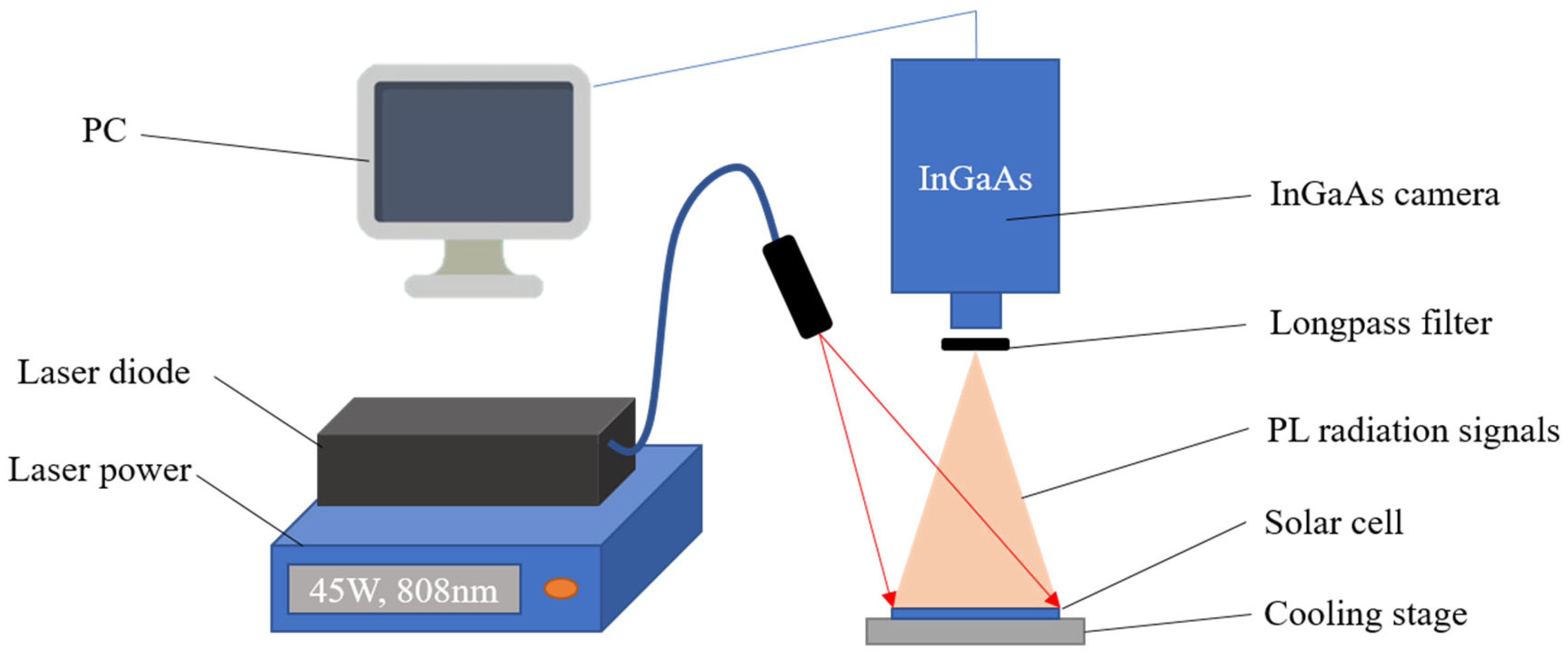
According to this principle, a PL detection system was established, which is shown in Figure 1. A DC laser system (808 nm, 45 W) was used to excite the sample, and an InGaAs camera (900~1700 nm) was used to capture the radiation signals. To block the reflection laser beam, a long-pass filter (1000 nm) was employed. A cooling stage was used to keep the sample in the room temperature range. All 5800 PL images were collected using the mentioned system.

Figure 1. PL detection system.

2.2. Definition and Grading of Defects in Photoluminescence Feature Images

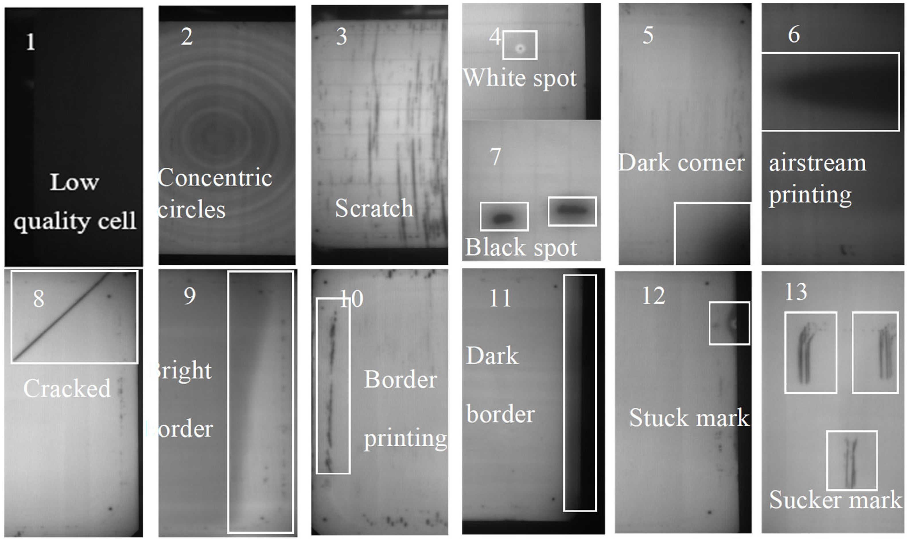
As the definition of defects in solar cells is not standardized yet, the features of different defects may be extremely similar (as shown in Figure 2). Therefore, it is necessary to define each category and the grades of each category [19]. This paper proposed a standard of defining defects in 13 categories and 3 sub-grades of each for solar cells. All types of defects are presented in Figure 2.

Figure 2. Types of solar cell defects.

2.2.1. Large Target Defect

Typically, the features of large target defects were clearer and easier to be annotated, which is suitable for the network model to detect. Low-quality cells, Concentric circles, Airstream printing, Bright borders, and Dark borders are defined as large target defect types.

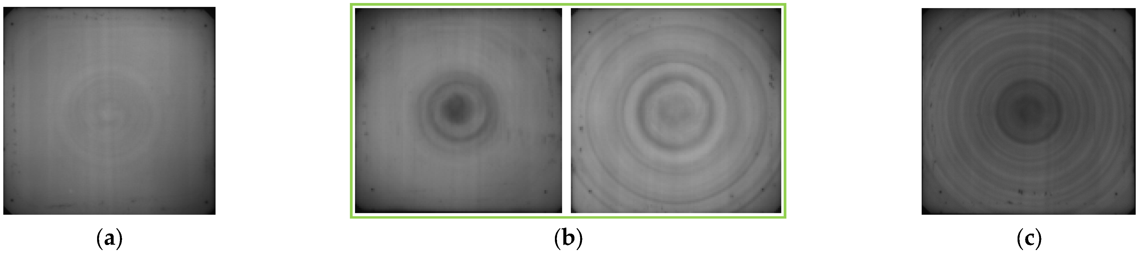
As for the gray mean of the PL grayscale feature image of cells less than 70, it was defined as a low-quality cell and marked as dark, which is unnecessary to grade according to the manufacturing requirements. For the other 3 defect types, Table 1 shows the criteria of classification and grading for several large target defects. Figure 3 describes the classification of Concentric circle defects. The 3 defect levels have different standards; these 3 levels completely cover all defects and are evenly distributed. Therefore, the grading standards of Airstream printing, Bright border, and Dark border defects are the same as Concentric circles.

Table 1. Classification and grading definition of large target defects.

Name	Grade	Grading Standard
		Position	Gray Mean of Defect	Relative Surface Area Filling
Concentric circle	Grade 1	Center	90~150	0.3~0.6
	Grade 2		90~150 30~90	0.6~1.0 0.3~0.6
	Grade 3		30~90	0.6~1.0
Airstream printing	Grade 1	Extend from a boundary to the whole surface	100~150	0.3~0.6
	Grade 2		100~150 50~100	0.6~0.9 0.3~0.6
	Grade 3		50~100	0.6~0.9
Bright border	Grade 1	A certain boundary	180~210	0.05~0.15
	Grade 2		210~240 180~210	0.15~0.25 0.05~0.15
	Grade 3		210~240	0.15~0.25
Dark border	Grade 1	A certain boundary	80~120	0.05~0.15
	Grade 2		80~120 30~80	0.15~0.30 0.05~0.15
	Grade 3		30~80	0.15~0.30

Figure 3. Grading of Concentric circle defect. (a) Grade 1; (b) Grade 2; and (c) Grade 3.

2.2.2. Small Target Defect

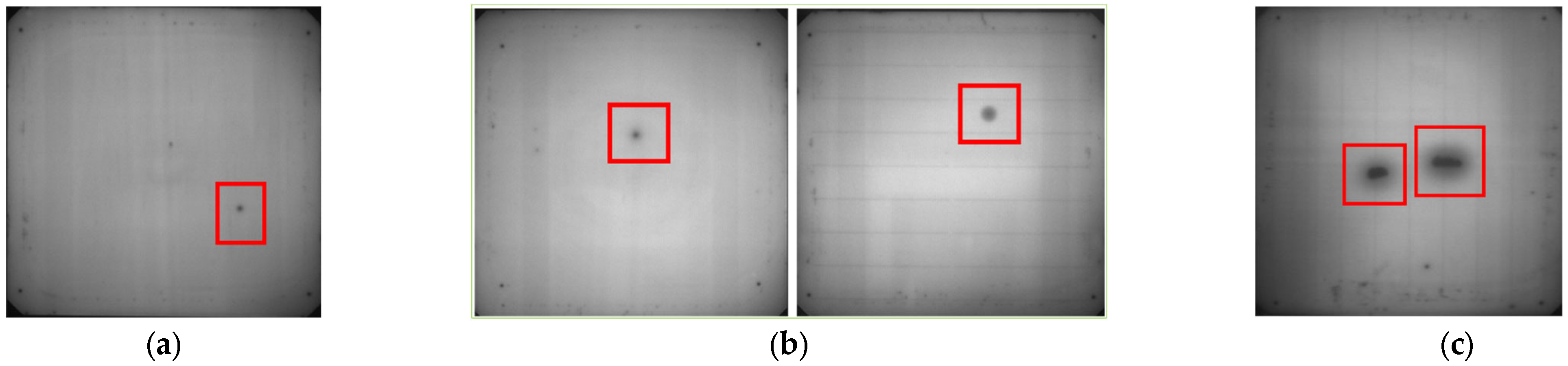
Compared to the large defects with clear features, the position of small defects is more random and lacks regularity. Due to the smaller size of defects that would be covered by background noise, it is necessary to find a suitable boundary for eliminating defects that do not affect battery performance. Black spot [20], White spot, Sucker mark, and Stuck mark were therefore defined as small defects. For the Black spot defect, definitions are made based on the different defect shape and size. Since the size of small defects is very small, the relative surface area filling degree cannot be used for screening, and the maximum radial length of a single defect is selected for characterization. Table 2 shows the criteria of the classification and grading for several small defects. Figure 4 shows the grading of Black spot defects.

Table 2. Classification and grading standards for small target defects.

Name	Grade	Grading Standard
		Position	Gray Mean of Defect	Maximum Radial Length/Pixels
Black spot	Grade 1	Random	80~120	1.0~3.0
	Grade 2		80~120 30~80	3.0~6.0 1.0~3.0
	Grade 3		30~80	3.0~6.0
White spot	Grade 1	Random	180~210	1.0~3.0
	Grade 2		210~240 180~210	3.0~6.0 1.0~3.0
	Grade 3		210~240	3.0~6.0
Sucker mark	Grade 1	—	100~150	3.0~7.0
	Grade 2		100~150 50~100	7.0~12.0 3.0~7.0
	Grade 3		50~100	7.0~12.0
Stuck mark	Grade 1	A certain boundary	90~150	7.0~12.0
	Grade 2		90~150 30~90	12.0~20.0 7.0~12.0
	Grade 3		30~90	12.0~20.0

Figure 4. Grading of black spot defects. (a) Grade 1; (b) Grade 2; and (c) Grade 3.

2.2.3. Complex Feature Defects

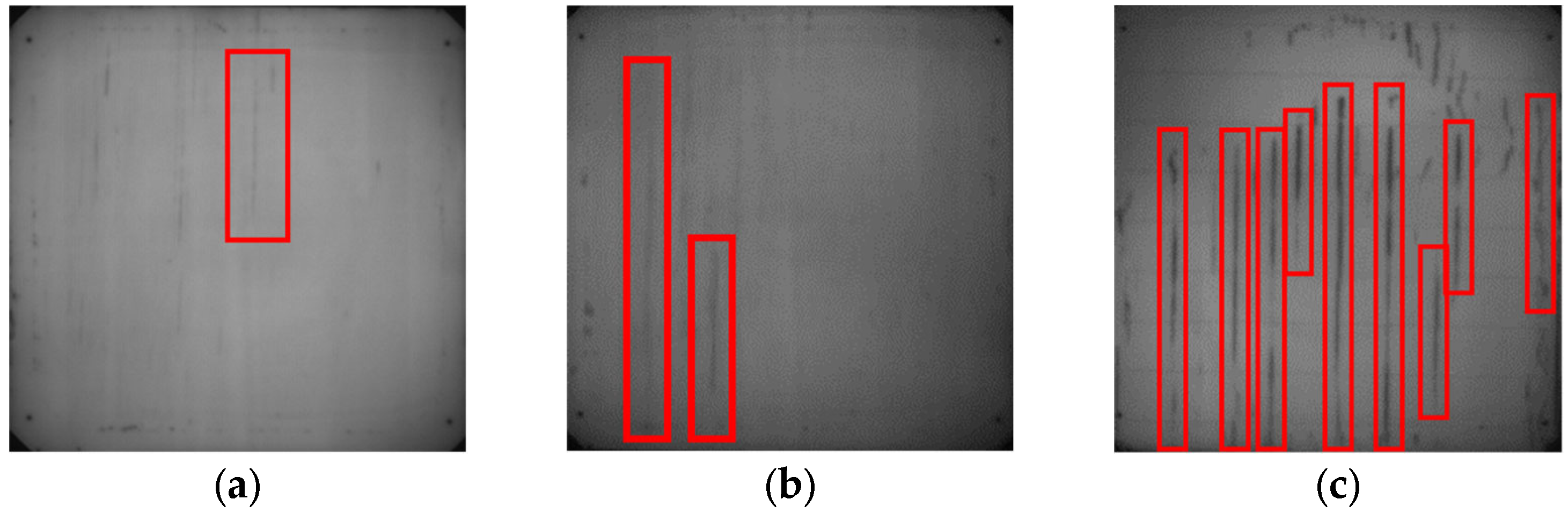
For the complex-type features, including Scratch, Border printing, Dark corner, and hidden crack defects [20], it is a challenge of the model to distinguish similar features of two overlapped defects in some samples. This greatly reduces the recognition and classification accuracy of the model for overall defects. Therefore, it is necessary to impose strict restrictions on the definitions of these two types of defects and different grades. For such circumstances, its randomized distribution of position and size was frequently accompanied by several scratch defects with similar features in the vertical direction, and was classified as a single defect with identically featured scratch defects within a 3-pixel distance.

The defects were then classified based on their radial length and the gray value of the defect location. Table 3 provides the classification and grading standards for complex-type defects, and Figure 5 provides the grading for scratch defects.

Table 3. Classification and grading standards for complex-type defects.

Name	Grade	Grading Standard
		Position	Gray Mean of Defect Location	Radial Length/Pixels
Scratch	Grade 1	Random	90~150	10~40
	Grade 2		90~150 30~90	40~70 10~40
	Grade 3		30~90	40~70
Border printing	Grade 1	Less than 40 pixels from the battery border	100~150	20~50
	Grade 2		100~150 50~100	50~80 20~50
	Grade 3		50~100	50~80
Dark corner	Grade 1	A certain corner	80~120	0.05~0.20
	Grade 2		80~120 30~80	0.20~0.35 0.05~0.20
	Grade 3		30~80	0.20~0.35
Hidden crack	Grade 1	Extending from a certain boundary, typically as a straight line or slightly curved arc

Figure 5. Grading of scratch defects. (a) Grade 1; (b) Grade 2; and (c) Grade 3.

2.3. Image Pre-Processing

PL images of solar cells contain noise, which increases the difficulty of feature extraction for neural networks. Therefore, it is necessary to pre-process the acquired images to improve the signal-to-noise ratio (SNR) of the feature images.

2.3.1. Contrast Enhancement

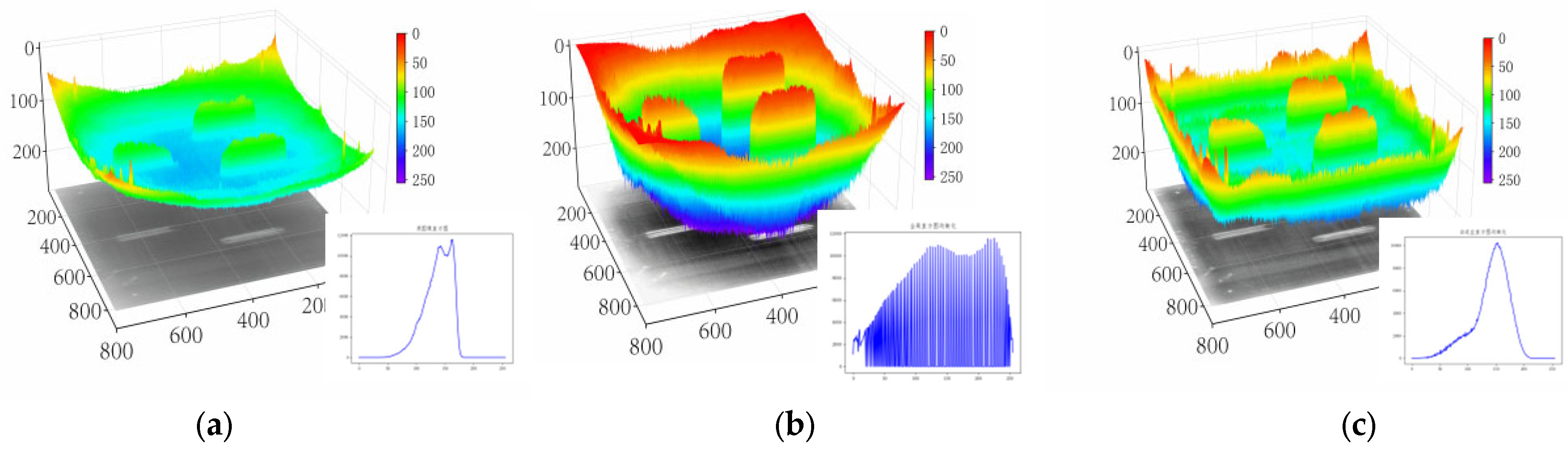
Histogram equalization can effectively enhance contrast. Both global histogram equalization and adaptive histogram equalization are used and compared. Figure 6 shows the original image and the contrast-enhanced result after processing.

Figure 6. The contrast-enhanced gray PL image. (a) Original feature image, (b) global histogram equalization, and (c) adaptive histogram equalization.

The grayscale 3D images in Figure 6 facilitate the observation of defects relative to the background. As shown in Figure 6b, defects could be well extracted, while the global histogram equalization enhance defect and noise together and differ the contrast significantly. The edge information of the PL image at the bottom of the 3D figure is lost due to global equalization. Compared with global histogram equalization, adaptive histogram equalization well extracted defect features and balanced edge information preservation, which well retained original features and smoothed out the regions with large grayscale changes

2.3.2. Image Filtering

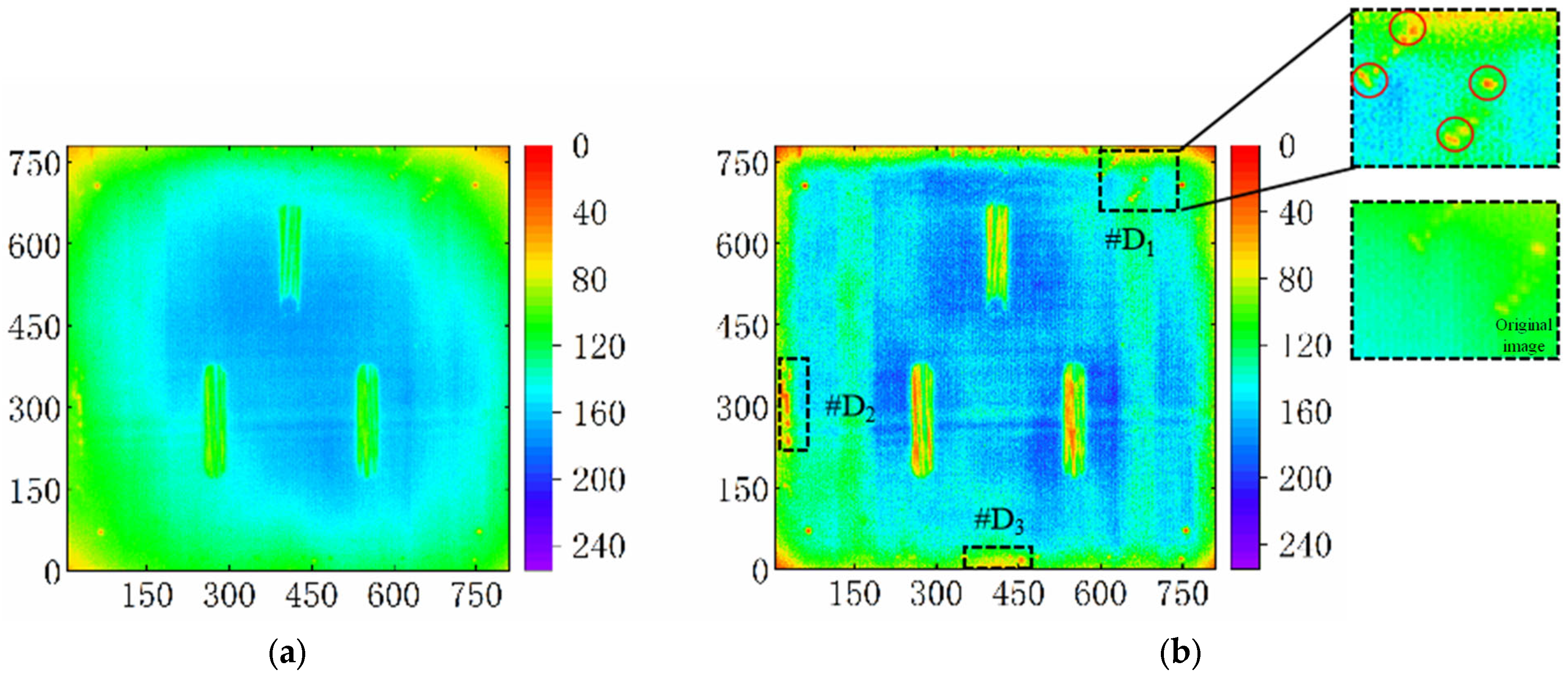
Histogram equalization can make the background noise more prominent, which can affect the quality of the image and the results of defect recognition. Figure 7 shows the original image and the image after contrast enhancement.

Figure 7. Noise enhancement caused by contrast enhancement. (a) Original feature image, and (b) contrast-enhanced image.

Figure 7, #D1, #D2, and #D3 show an amplification of subtle noise under the contrast enhancement, where the noise filter was necessarily required. It is necessary to apply filtering to eliminate the noise. Gaussian and median filtering were used to process the image and their results were compared.

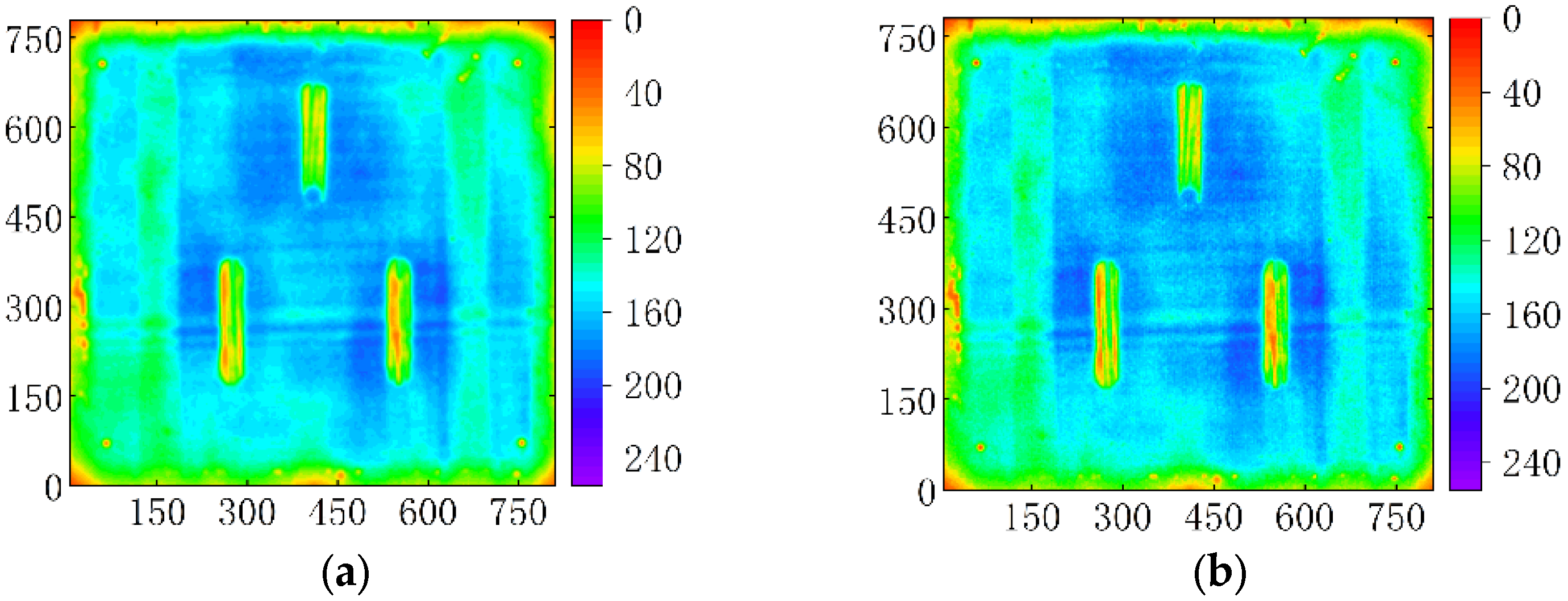
Figure 8 shows that both methods were able to filter and eliminate noise, while the Gaussian filtering effectively smoothed the image and suppressed the background noise other than median filtering. However, the effect of median filtering is worse than that of Gaussian filtering, and Gaussian filtering effectively smoothed the image and suppressed the background noise. Therefore, Gaussian filtering was chosen to remove the noise.

Figure 8. Comparison of Gaussian and median filter processing results. (a) Gaussian filtering; (b) median filtering.

2.3.3. Feature Image Segmentation

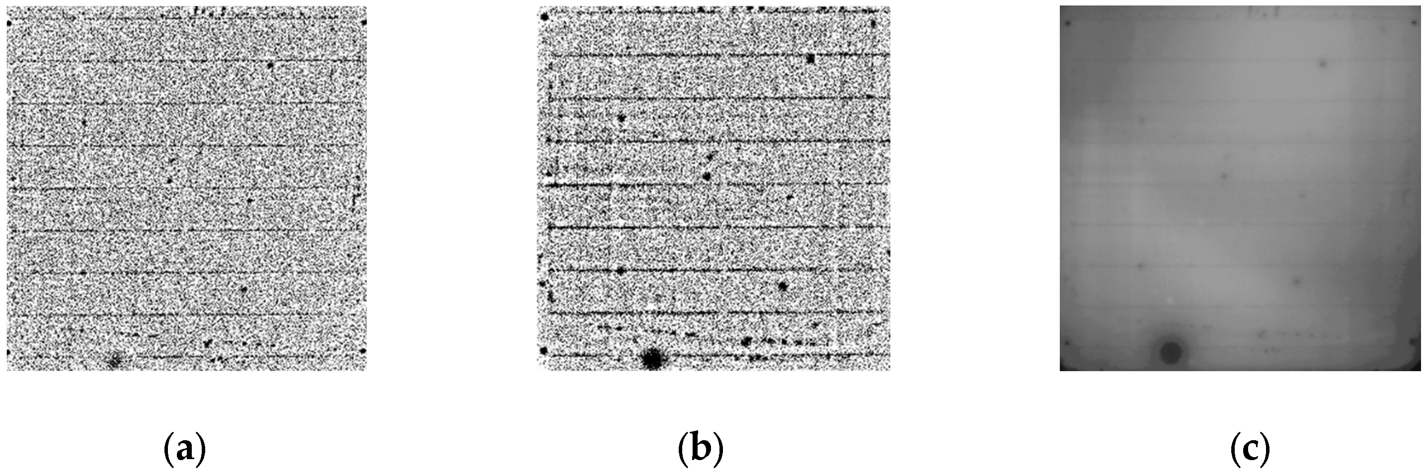
Separating defects from the background of sample images is beneficial for neural network recognition. As solar cell defects may exhibit features with opposite color values, such as White spot, Black spot, Dark cell, and Bright border, common methods, such as binarization, are difficult to use for defect segmentation. This paper uses neighborhood weighted mean adaptive threshold segmentation (NWM-ATS), neighborhood weighted Gaussian adaptive threshold segmentation (NWG-ATS), and K-means clustering segmentation to compare their results, as shown in Figure 9, for the processed feature images, using the three methods.

Figure 9. Comparison of image segmentation results. (a) NWM-ATS, and (b) NWG-ATS, (c) K-means clustering segmentation.

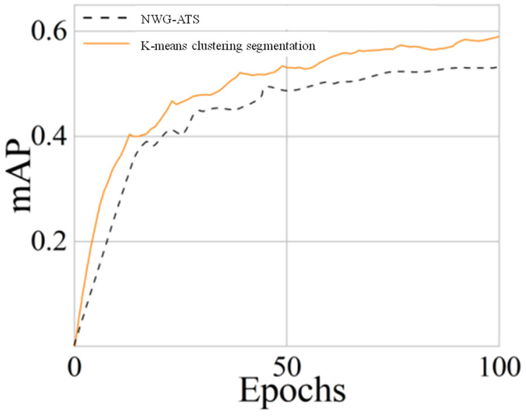
According to Figure 9, all three methods can separate the defect target from the background, but NWM-ATS blurs a part of the defect, and causes original feature loss of the image. Figure 10 shows the 50-epoch training that was carried out on a small amount of images processed by NWG-ATS and K-means cluster segmentation. It can be seen that after 50 epochs of iteration, the mAP of K-means clustering segmentation reaches 60%, while that of NWG-ATS is lower than 50%. Therefore, K-means clustering segmentation is used for image segmentation.

Figure 10. The mAP curve of NWG-ATS and K-means clustering segmentation.

2.4. Data Augmentation

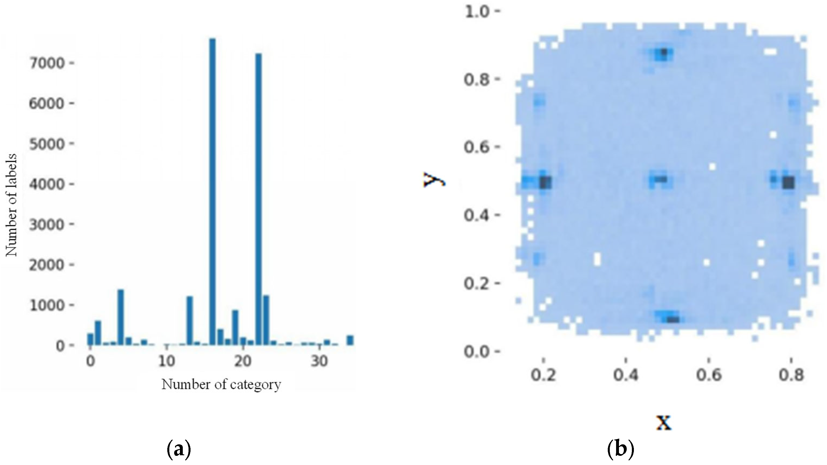
The previous section describes the preprocessing of defect images and the definition of defects. The Labelimg software was used to label the defect of the obtained PL image dataset, and the number of defect labels for each defect category was counted. Figure 11 shows the distribution of the number and location of defects at each grade for each defect category.

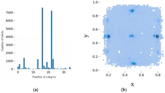
Figure 11. The distribution of the number and location of defects for each defect category. (a) Distribution of the number of categories; (b) distribution of defect positions.

As illustrated by Figure 11, the number of some defect samples is sufficient or even more than 7000, but the number of samples for some defect categories is less than 50. This can lead to incomplete feature information for this category of defects, which can reduce the recognition accuracy of the network model for this type of defect and thus affect the overall detection accuracy. Therefore, in order to achieve better recognition performance for a particular type of defect, the sample size for that type of defect should be at least 400. In order to enrich the dataset and improve the ability of the neural network to identify each defect category and sub-grade, data augmentation is required.

2.4.1. Mosaic Data Augmentation

Commonly used data augmentation methods for original data can be divided into two categories: color space transformation and two-dimensional coordinate transformation [21]. Color space transformation involves transforming the RGB color space into the HSV color space, which is composed of hue (H), saturation (S), and value (V) [22]. Color space transformation is accomplished by hue transformation, saturation transformation, brightness transformation, and transparency transformation. Two-dimensional coordinate transformation utilizes plane spatial processing such as flipping and cropping to change the spatial position and shape features of the target object to achieve the goal of data augmentation.

Color space transformation can enrich the data sample to a certain extent. However, since the PL feature image is based on the grayscale space dataset, hue, saturation, and brightness changes have no significant effect. Two-dimensional coordinate transformation cannot simultaneously reverse the label position when reversing the original image. The mosaic algorithm [23] randomly divides certain regions and merges them with other images with random scales and sizes, thereby improving the generalization ability of the trained neural network to feature information. In addition, the mosaic algorithm ensured the defect marking information was synchronized with original image during splicing when processing images, delivering more reliable data augmentation results. The principle of the mosaic algorithm is to randomly select four images from the dataset and splice them with random scales. The principle is as follows:

$$\tilde{x}=M\odot x_A+\left(1-M\right)\odot x_B$$

(3)

$$\tilde{y}=\mathsf{\lambda }{y}_A+\left(1-\mathsf{\lambda }\right)y_B$$

(4)

where x represents the training image, y represents the label, and λ represents the combination ratio between the two samples, where λ∈(0,1).

Figure 12 presents the feature image obtained using the mosaic algorithm.

Figure 12. The feature images obtained using the mosaic algorithm.

2.4.2. Mixup Data Augmentation

Owing to the recently increasing depth of neural networks, the sensitivity to adversarial samples remained unsatisfied. Using Mixup [24] can mitigate this problem. Essentially, this method changes the representation of the defect target at different scales, resulting in training samples with better linear structure and more enriched feature information for each category. This can improve the generalization performance of the current state-of-the-art neural network architecture and effectively reduce the interference of partially mislabeled results caused by similar defect features. The definition of Mixup is as follows:

$$\tilde{x}=\mathsf{\lambda }{x}_i+(1-\mathsf{\lambda })x_i$$

(5)

$$\tilde{\mathrm{y}}=\mathsf{\lambda }{y}_i+(1-\mathsf{\lambda })y_i$$

(6)

where x_i represents the randomly selected image from the training set, y_i represents the label corresponding to the randomly selected image, and λ represents the combination ratio between the two samples, where λ ∈ (0, 1).

Mixup can be combined with the mosaic algorithm by adding Mixup calculations to the process of randomly selecting and combining four images in the mosaic method. Figure 13 shows the dataset processed by the mosaic and Mixup methods.

Figure 13. The feature images obtained using mosaic and Mixup methods.

2.4.3. Copy–Paste Data Augmentation

The above two data augmentation methods greatly expanded the original data samples, except the recognition of 39 types of defects in the existing dataset, and the desired results were still considered as a small data sample size. Therefore, it is necessary to find data augmentation methods suitable for solar cell identification to further expand the data samples as much as possible.

The 39 types of defects on the PL feature images of solar cells are randomly distributed. Therefore, the copy–paste [25] can be used to simulate the random occurrence of defects during the production of solar cells. The main idea of this method is to combine Mixup and large-scale jittering (LSJ) [26]. Mixup can be defined as follows:

$$\tilde{I}=\alpha I_1+(1-\alpha )I_2$$

(7)

where I₁ and I₂ are randomly selected images from the training set, α is the mixing ratio between the two samples, α ∈ (0, 1). In other words, some pixels in the image I₂ are copied and pasted into the image I₁, and this process has a high degree of randomness.

LSJ is a bolder scale jittering method compared to standard-scale jittering (SSJ) [27]. In SSJ, the scale variation ranges from 0.8 to 1.25, while in LSJ, the scale variation range is from 0.1 to 2.0. A wide range of jittering leads to a strong contrasting jittering effect. Additionally, both LSJ and SSJ use random horizontal flipping.

By randomly scaling I₁ and I₂ feature images, and randomly mixing and pasting the feature defect pixels from I₁ and I₂, copy–paste can simulate the random occurrence of defects in solar cells during production.

2.4.4. Combination of Data Augmentation Algorithms

By combining the three data augmentation methods, the mosaic method provided a 1 times data augmentation increment, where the other two provided 0.1 and 0.5 times for Mixup and copy–paste, respectively. Simultaneously, the batch size of input images was set to 8 for training process speed up, which is correspondingly shown in Figure 14.

Figure 14. The feature images obtained using mosaic, Mixup, and copy–paste.

2.5. Photoluminescence Fusion Convolution Neural Network for Solar Cell Defect Detection

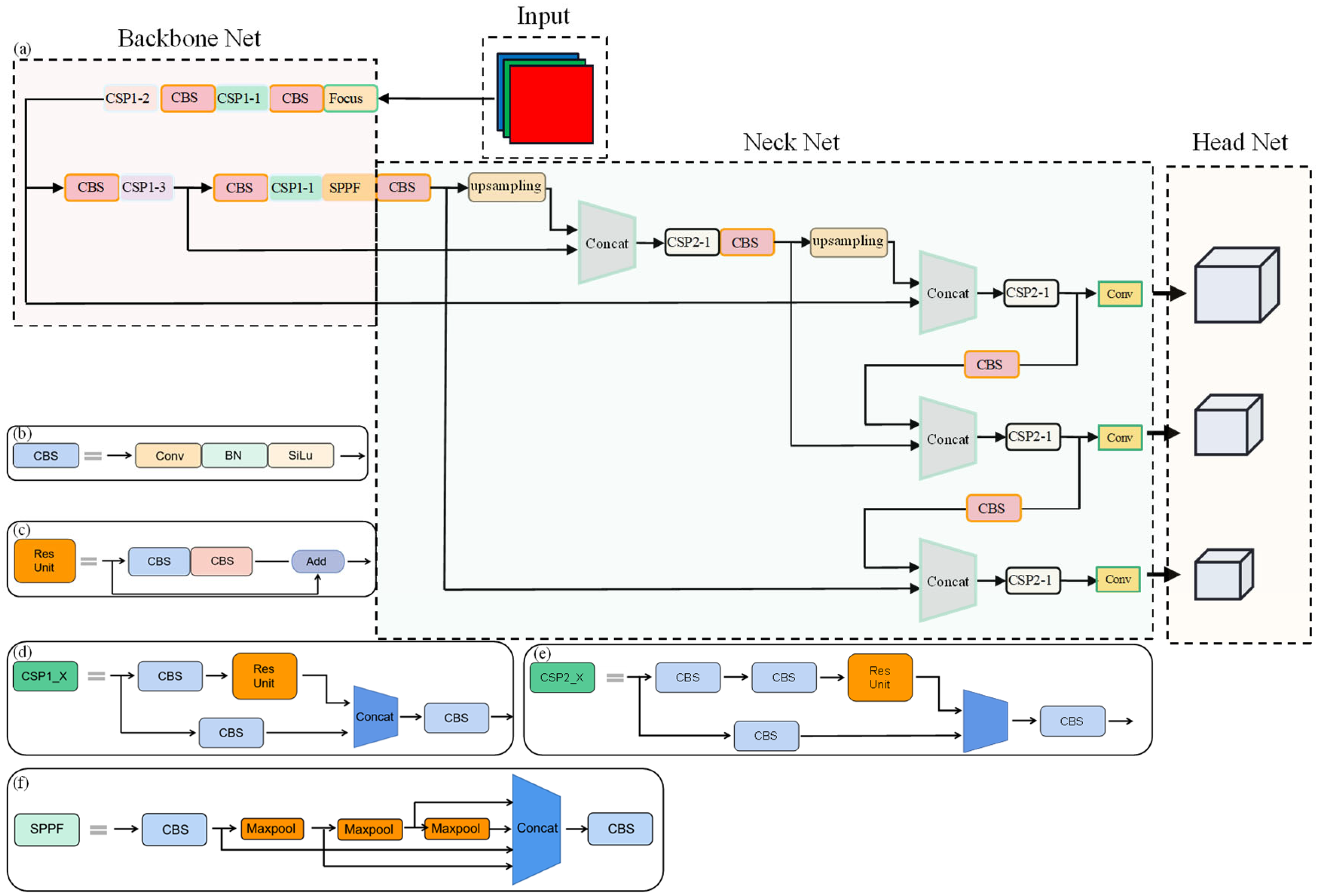
Combining the basic structure of the YOLOv5 neural network and the characteristics of solar cell defect recognition, a neural network model structure as shown in Figure 15 was built. YOLOv5 consists of three parts: backbone net, neck net, and head net.

Figure 15. Illustration of the YOLO model structure. (a) Yolo; (b) CBS model; (c) Res Unit model; (d) CSP1_X; (e) CSP2_X; (f) SPPF.

2.5.1. Backbone Net

The network structure under backbone net consisted the focus module, the CBS module, the cross stage partial block net (CSP net) [28], and the spatial pyramid pooling–fast (SPPF) [29].

The focus module is used to achieve down-sampling of the original image while preserving a large amount of target position information and feature information. After obtaining the feature image, a convolution calculation is performed on the image, and batch normalization (BN) [30] and activation functions are required. The CBS module is composed of convolutional layers, BN layers, and SiLU activation functions, and is used as the basic structure of the neural network. Its structure is shown in Figure 15b.

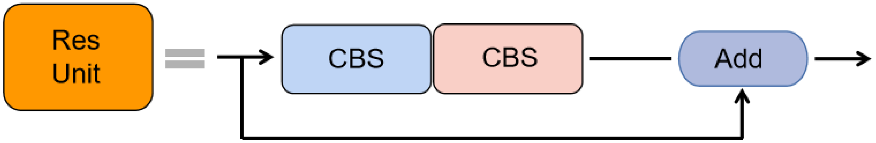
In order to alleviate the redundancy in gradient computation caused by weight updates in back-propagation, CSP net is added to the backbone net to reduce the computation redundancy. With the inspiration of the residual network, two tensors of different scales at corresponding stages that were formed by insertion of residual units between input and output would concatenate and fuse the feature mapping from input to output. The structure diagram of the residual unit is shown in Figure 16. The CSP net consisting of residual units, CBS module, and feature fusion module mainly exist in the model formed as CSP_X, representing the number of residual units. Figure 15d,e shows the structural diagram of the CSP_X module.

Figure 16. Residual unit.

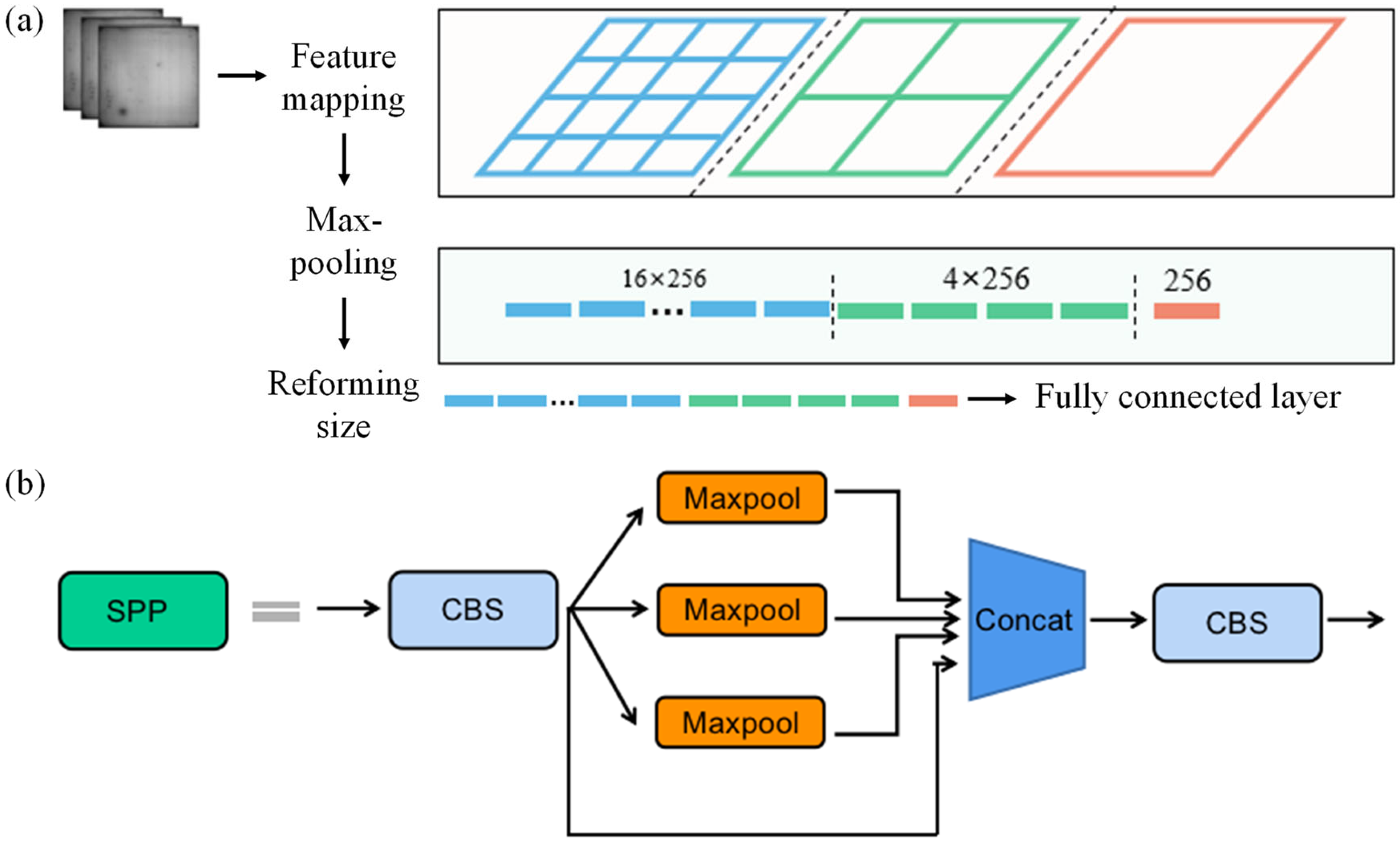
The backbone net has the function of handling images with a unified input size, and the resize operation may lead to the loss of image information. However, the spatial pyramid pooling (SPP) structure can solve this problem. Firstly, the arbitrarily sized images are input to the convolutional layer to extract feature information, which is divided into 4 × 4, 2 × 2 and 1 × 1 parts; that is, the feature maps are divided into 16 × 256, 4 × 256, and 1 × 256 parts, respectively. Secondly, the max-pooling operation is applied to resize the feature map to the required size, and the information is input into the neck net through a fully connected layer. The principle and structure of the SPP module are shown in Figure 17.

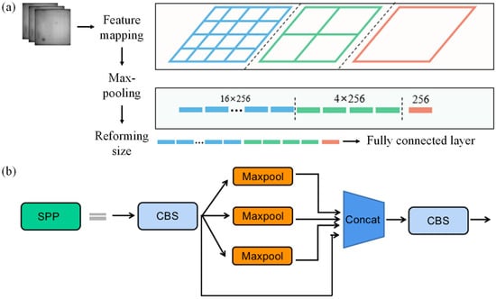
Figure 17. The principle and structure of the SPP module. (a) The principle of the SPP module. (b) The structure of the SPP module.

SPP consumed a large amount computation on performing three paralleled max-pooling operations on feature maps according to different sizes and combining four different sizes of feature information via multi-scale fusion. To address this issue, a fast spatial pyramid pooling structure (spatial pyramid pooling–fast, SPPF) is used, as shown in Figure 15f. Compared with the SPP module structure, the SPPF module concatenates max-pooling operations to reduce computational complexity while ensuring performance. Therefore, this paper will use the SPPF structure as the module for adjusting the input feature map size.

2.5.2. Neck Net

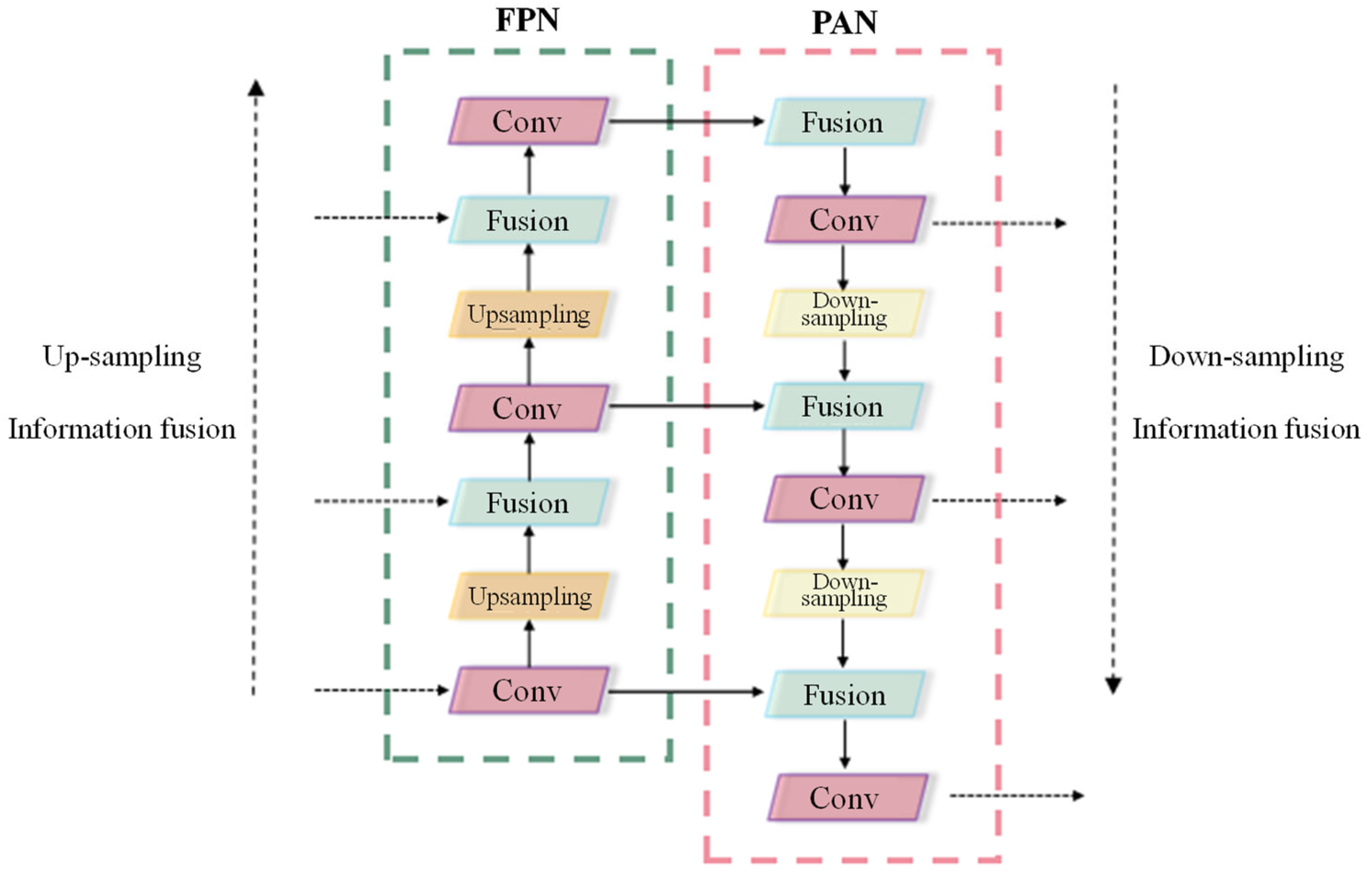
The characteristic information of defects in solar cells is complex, covering both large and small targets. For the recognition of large-scale targets, more down-sampling is needed to ensure a larger receptive field for extracting a larger range of feature information. For the recognition of small-scale targets, less down-sampling is needed to ensure a smaller receptive field for extracting small target information. Therefore, information fusion and the transmission of features at different scales are needed. Thus, the entire structure of the neck net is mainly constructed by combining FPN [31] and PAN [32], which enables feature information at different scales to be well reserved and fused to prevent information loss during convolution and pooling processes. Figure 18 shows the neck net structure based on FPN and PAN. The FPN algorithm is a bottom-up propagation path, whereas the PAN presented, contrarily, that a more abundant semantic of the feature map could be obtained under lateral connection-based feature fusion.

Figure 18. Neck network structure based on FPN and PAN.

2.5.3. Head Net

In head net, since 3 detection boxes are generated for each target region, one of the detection boxes that can best recognize the target is selected to fit the actual position information of the target, and the remaining detection boxes are discarded. This process requires using non-maximum suppression (NMS) [33] to grade the 3 detection boxes generated by the model and keep the one with the highest score.

During training, it is necessary to use loss functions to reflect the actual differences and feedback this information to the backpropagation process to obtain the error of each layer and update the weights of each layer so that the prediction results of the final layer gradually approach the true values. The losses of the model mainly include the position loss of the predicted box, the confidence loss of target recognition, and the category loss.

Currently, the commonly used position loss functions for predicting bounding boxes are IoU, GIoU, DIoU, and CIoU [34]. Among them, CIoU loss is used as the loss function for predicting box positions. By increasing the loss of the scale and length–width ratio of the detection box, the predicted box of the model can be closer to the real box. For the multi-classification problem in this paper, many category and grade features are very similar to each other. Therefore, the sum of the category feature vectors of the predicted boxes obtained by the softmax classifier is prospectively unnecessarily equal to 1; that is, a target can belong to multiple categories at the same time, and the one with the highest confidence is selected. Based on this idea, BCE with logits loss [35] is used as the loss function for category and confidence loss. This loss function met the above requirement and further balanced the contrast samples of the category and improved the robustness of the network model.

3. Results and Analysis

To train the neural network for PL images, the label–image module was used to label the category and position information of the pre-processed PL feature images according to the defect classification grading definition. A total of 7311 defect targets were labeled. A Dell desktop workstation with an Intel Core i9-10980X CPU, NVIDIA GeForce RTX 3090 GPU with 24 G RAM, 256 GB RAM, and Windows 10 64-bit OS was employed for YOLOv5 model training and testing. Homemade software was programmed using Python 3.8, CUDA11.3, and the deep learning framework was established based on Pytorch 1.11.0.

In order to observe the variation rule of the neural network during the training process, precision and recall were defined as evaluation metrics for the model with the following formulas:

$$precision=\frac{TP}{TP+FP}$$

(8)

$$recall=\frac{TP}{TP+FN}$$

(9)

the relationship between TP, FP, and FN in the equation is shown in Table 4. AP is defined as the area under the precision–recall (P-R) curve. When recognizing and detecting multiple types of objects, the sum of the APs for all categories is the mean average precision (mAP), which can reflect the overall performance of the training and recognition process.

Table 4. Confusion matrix.

Reference	Prediction
	Positive	Negative
Positive	TP	FN
Negative	FP	TN

3.1. Hyperparameter Tuning

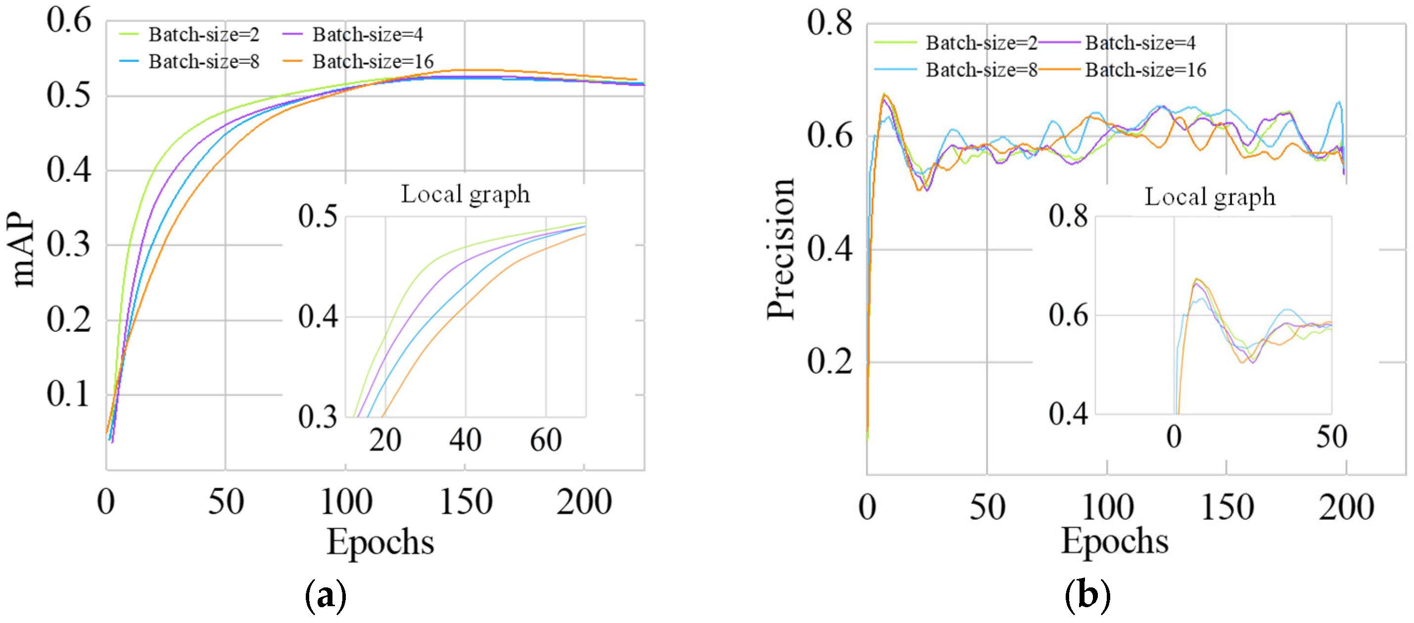
The hyperparameters that need to be modulated include batch size, epochs, and image size, and the experimental parameters are shown in Table 5. In the experiments, epochs = 200 and image size = 480 × 480 were used, and mAP and precision were used as evaluation metrics for model training. Figure 19 shows the change curves of mAP and precision for different batch sizes.

Table 5. Modulation parameter setting.

Hyperparameter	Value
Batch size	2, 4, 8, 16
Epochs	200
Image size	480

Figure 19. Comparison of training results with different batch size. (a) mAP Curve with epoch; (b) precision curve with epoch.

From Figure 19a, mAP of different batch sizes is basically stabilized and converged after 150 epochs, and the main difference is that the larger the batch size, the faster the convergence of mAP for defects. From Figure 19b, it can be seen that changing the batch sizes has little effect on the change in precision. Table 6 compares the optimal results of the network model indicators under different batch sizes within 200 epochs. As Table 6 shows, four indicators, including precision, recall, mAP_0.5, and mAP_0.5:0.95 remained stable with the increasement of batch size, yet led to gradual increase in VRAM occupancy and a gradual decrease in training time under the same epoch. This indicates that increasing the batch size will effectively increase the experiment rate for computer hardware, shorten the training time, and improve experimental efficiency.

Table 6. Different training results of YOLOv5 under different batch size.

Evaluation Indicators	Precision	Recall	mAP0.5	mAP0.5:0.95	Training Time (h)	VRAM (G)
Batch size = 2	0.572	0.601	0.536	0.309	35.16	3.2
Batch size = 4	0.569	0.601	0.533	0.309	20.21	8.2
Batch size = 8	0.542	0.603	0.535	0.31	13.37	12.1
Batch size = 16	0.572	0.607	0.549	0.315	11.28	16.2

VRAM usage reached 16.2 G while the batch size was set to 16, and the actual available VRAM was 20.1 G due to hardware platform limitations. To reserve enough space, this article chooses a batch size of 8. The principles for selecting epochs and image size are the same as for batch size, taking into account the impact on model training results, training time control, VRAM usage of the hardware system, etc., so epochs = 200 and image size = 480 × 480 are selected.

3.2. The Effect of Pretreatment on Recognition Accuracy

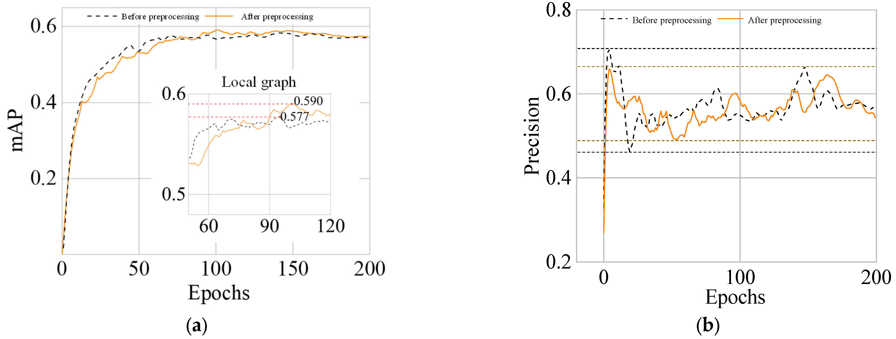
The main parameters of the experiment are batch size = 8, IoU threshold = 0.2, momentum = 0.937, image size = 480 × 480, and epochs = 200. Figure 20 shows the changes of mAP and precision curves obtained by experiments in 200 epochs when the feature image is preprocessed and not preprocessed.

Figure 20. Comparison of results with and without preprocessing. (a) mAP Curve with epoch; (b) precision curve with epoch.

From Figure 20a, the mAP of the model was improved by 1.3% after the feature images were preprocessed. From Figure 20b, the precision curve of the model converges faster and fluctuates less, indicating that the training inference speed of the model is improved for targets with clearer features. Table 7 presents the changes in various evaluation indicators of the neural network before and after preprocessing. From the table, image preprocessing did not increase training time and VRAM usage, but significantly improved four indicators. Therefore, using image preprocessing can effectively improve the recognition ability of defects.

Table 7. Changes in evaluation metrics of the neural network before and after preprocessing.

	Precision	Recall	mAP0.5	mAP0.5:0.95	Training Time (h)	VRAM (G)
Before preprocessing	0.542	0.603	0.577	0.31	13.37	12.1
After preprocessing	0.563	0.635	0.590	0.318	13.37	12.1
Improved	+3.9%	+5.31%	+4.49%	+2.58%	—	—

3.3. Analysis of Defect Recognition Performance for Different Target Categories

For better analysis of the recognition effect on the recognition effect of neural network structure on various types of defects, it is necessary to summarize the training results, including the target defect category, label number, precision, recall, mAP_0.5, and mAP_0.5:0.95. The naming convention for defect categories and grades is to add a number to the defect name (e.g., Concentric_circles01). Table 8 summarizes the information for each category. The recognition performance of each category and grade is rated based on precision, recall, mAP_0.5, and mAP_0.5:0.95. For example, Concentric_circles03, Black_spot03, and Dark_corner03 all have a mAP_0.5 of over 90%, so their defect grade is rated as A. Cracked, Concentric_circles01, Concentric_circles02, Stuck_mark02, Stuck_mark03, Sucker_mark01, and others have a mAP_0.5 between 60% and 80%, so their defect grade is rated as B. Dark_border01, Sucker_mark02, White_spot02, and others have mediocre performance in mAP_0.5, mAP_0.5:0.95, recall, and precision, with mAP_0.5 between 40% and 60%, so their defect grade is rated as C. Scratch01, Scratch02, Scratch03, Border_printing01, Dark_border02, and others have a mAP_0.5 lower than 40%, so their defect grade is rated as D.

Table 8. Summary of training results for different categories.

Defect Category	Number	Precision	Recall	mAP0.5	mAP0.5:0.95	Grade
Cracked	161	0.652	0.658	0.691	0.422	B
Concentric_circles01	198	0.609	0.808	0.753	0.453	B
Concentric_circles02	31	0.624	0.71	0.614	0.385	B
Concentric_circles03	44	0.746	0.937	0.929	0.734	A
Stuck_mark01	361	0.445	0.546	0.398	0.113	D
Stuck_mark02	84	0.533	0.643	0.644	0.32	B
Stuck_mark03	13	0.461	0.692	0.654	0.28	B
Dark_border01	31	0.458	0.645	0.474	0.251	C
Dark_border02	4	0.963	0.25	0.372	0.193	D
Dark_border03	2	1	0	0	0	D
Sucker_mark01	16	0.572	0.812	0.798	0.344	B
Sucker_mark02	9	0.456	0.667	0.561	0.295	C
Sucker_mark03	14	0.582	0.857	0.804	0.456	B
White_spot01	702	0.594	0.886	0.814	0.3	B
White_spot02	47	0.474	0.745	0.581	0.276	C
White_spot03	8	0.24	0.875	0.612	0.331	B
Border_printing01	1350	0.404	0.745	0.568	0.212	C
Border_printing02	227	0.516	0.714	0.609	0.337	B
Border_printing03	71	0.43	0.746	0.602	0.299	B
Black_spot01	317	0.386	0.565	0.483	0.162	C
Black_spot02	99	0.592	0.798	0.752	0.359	B
Black_spot03	68	0.877	0.941	0.963	0.479	A
Scratch01	2399	0.357	0.565	0.382	0.132	D
Scratch02	585	0.269	0.4	0.243	0.0936	D
Scratch03	92	0.257	0.087	0.0911	0.0321	D
Bright_border01	16	0.66	0.608	0.591	0.259	C
Bright_border02	41	0.726	1	0.929	0.471	A
Bright_border03	3	0.399	1	0.746	0.545	B
Airstream_printing01	33	0.686	0.606	0.563	0.332	C
Airstream_printing02	28	0.512	0.857	0.745	0.409	B
Airstream_printing03	16	1	0.551	0.762	0.518	B
Dark_corner01	92	0.492	0.304	0.348	0.133	D
Dark_corner02	15	0.132	0.267	0.073	0.0282	D
Dark_corner03	8	0.588	1	0.962	0.54	A
Low_cell	126	0.995	1	0.995	0.983	A

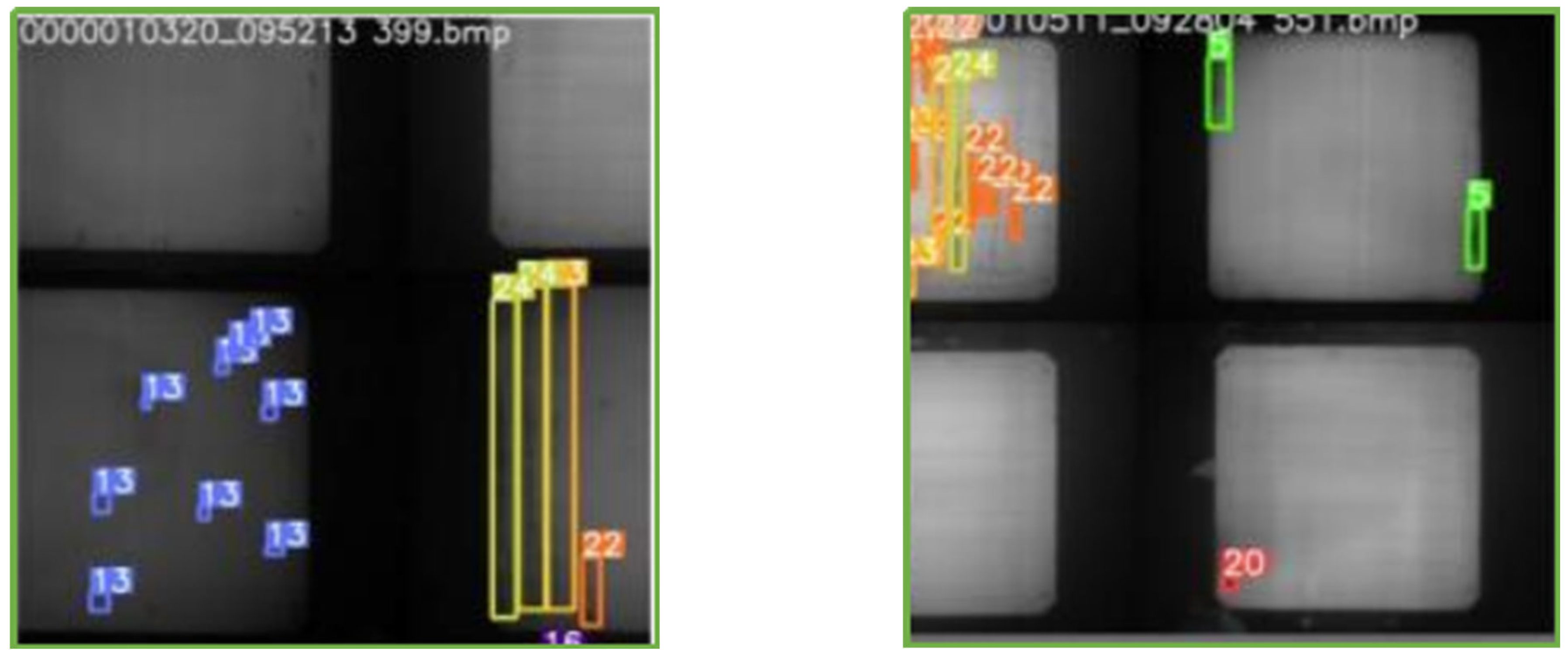
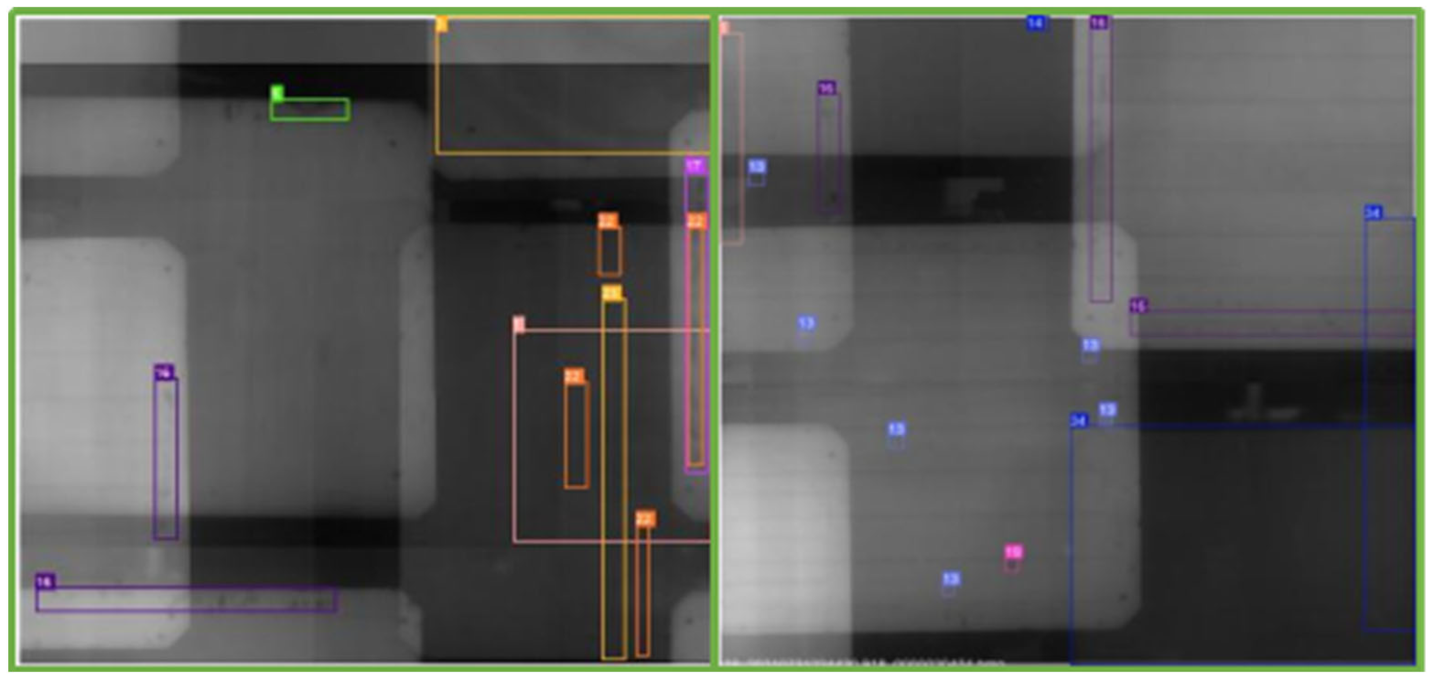
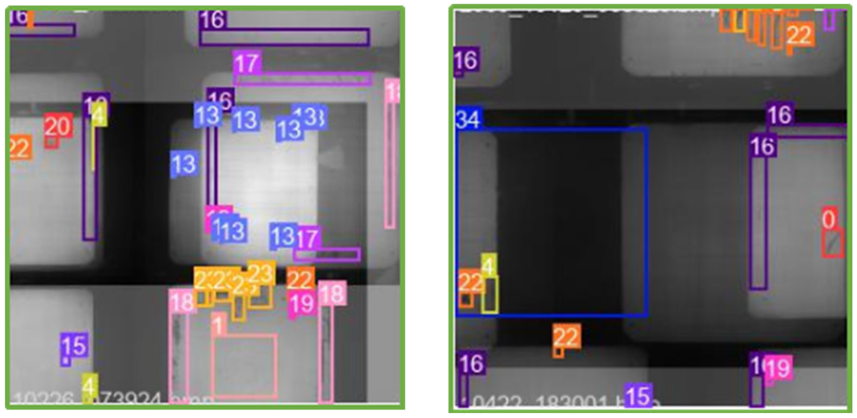
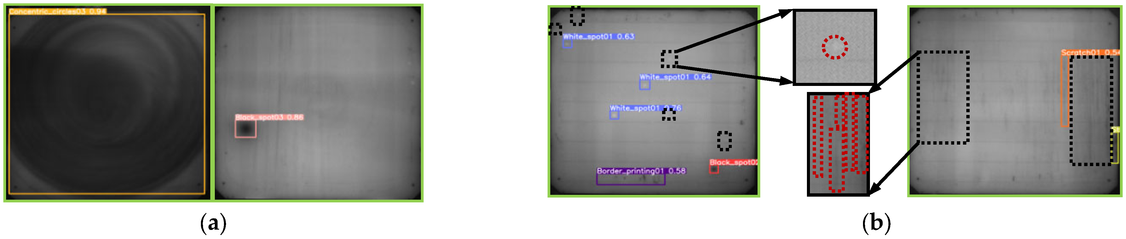
Figure 21 presents a comparison of the target defect recognition results. It shows that for defects that are too small or have indistinct features, it is easy to miss detection or make false alarms, seriously affecting the recognition effect of these types of defects.

Figure 21. Comparison of different defect recognition performance. (a) Well-recognized defects; (b) defects with missed detections.

Table 9 presents the analysis of the reasons for poor recognition results. It can be seen from the analysis that to improve the classification and grading ability of the model for poorly recognized targets, the ability to recognize small target defects and extract features of complex feature defects should be improved. For categories with insufficient samples and labels, they should be supplemented in future work.

Table 9. Analysis of the reasons for the poor recognition results.

Number	Reasons for Poor Recognition	Category
1	The size of small target defects is too small for neural network models to detect;	White_spot02, Black_spot01
2	Complex feature defects are difficult to distinguish from other defects;	Stuck_mark01, Border_printing01
3	Insufficient sample and label quantities, or difficulties in labeling can make it challenging to obtain complete feature information for corresponding defects.	Dark_border, Sucker_mark02, Bright_border01, Airstream_printing01, Dark_corner01, Dark_corner02, Scratch

4. Conclusions

This paper focused on the classification and grading of defects of semifinished silicon solar cells using the YOLOv5 model based on PL technology. Adaptive histogram equalization was used to enhance the distinction between target features and background information. Gaussian filtering was applied to suppress noise enhancement caused by contrast enhancement, and K-means clustering threshold segmentation was adopted to extract defect features. Thirteen major defect classification and grading rules for each defect were established, and defects were classified and graded based on the defect size, grayscale value, and position information, standardizing the marking process for solar cell defects. Image data augmentation was achieved via a combination of mosaic, Mixup, and copy–paste procedures that resulted in a more comprehensive PL image dataset. A neural network was pre-built based on the YOLOv5 model framework, attaching a more efficient SPPF module to replace the SPP module in the backbone network, while a CBS module based on the adaptive SiLU activation function replaced the CBL module in the CSP module, with the integration of FPN and PAN structures in the neck network. In the head network, NMS was used to select the target box closest to the real target, whereas the CIoU loss was used as the loss function for predicting box position information, and the BCE with logits loss was used as the loss function for classification and confidence. According to experimental analysis, the optimal combination of hyperparameters and the practical effect of data sample preprocessing on the training results of the neural network were determined. The cause of poor recognition effectiveness for small target and complex feature defects were identified on the foundation of the differences of categorizing and grading effectiveness, and future directions for work were proposed.

References

- Song, P.; Zhao, J.; Liu, J.; Yue, H.; Pawlak, M.; Sun, X. Evaluation of the performance degradation of silicon solar cell irradiated by low-level (<1 MeV) energetic particles using photocarrier radiometry. Infrared Phys. Technol. 2022, 123, 104177. [Google Scholar] [CrossRef]
- Mazalan, E.; Aziz, M.S.; Amin, N.A.; Ismail, F.D.; Roslan, M.S.; Chaudhary, K. First-principles study on crystal structures and bulk modulus of CuInX2 (X = S, Se, S-Se) solar cell absorber. J. Phys. Conf. Ser. 2023, 2432, 012009. [Google Scholar] [CrossRef]
- Sturm, F.; Trempa, M.; Schuster, G.; Hegermann, R.; Goetz, P.; Wagner, R.; Barroso, G.; Meisner, P.; Reimann, C.; Friedrich, J. Long-Term Stability of Novel Crucible Systems for the Growth of Oxygen-Free Czochralski Silicon Crystals. Crystals 2022, 13, 14. [Google Scholar] [CrossRef]
- Bhatt, V.; Kim, S.T.; Kumar, M.; Jeong, H.J.; Kim, J.; Jang, J.H.; Yun, J.H. Impact of Na diffusion on Cu (In, Ga) Se2 solar cells: Unveiling the role of active defects using thermal admittance spectroscopy. Thin Solid Films 2023, 767, 139673. [Google Scholar] [CrossRef]
- Jošt, M.; Kegelmann, L.; Korte, L.; Albrecht, S. Monolithic Perovskite Tandem Solar Cells: A Review of the Present Status and Advanced Characterization Methods Toward 30% Efficiency. Adv. Energy Mater. 2020, 10. [Google Scholar] [CrossRef]
- Tang, W.; Yang, Q.; Xiong, K.; Yan, W. Deep learning based automatic defect identification of photovoltaic module using electrolumines-cence images. Sol. Energy 2020, 201, 453–460. [Google Scholar] [CrossRef]
- Ai, L.; Yang, Y.; Wang, B.; Chang, J.; Tang, Z.; Yang, B.; Lu, S. Insights into photoluminescence mechanisms of carbon dots: Advances and perspectives. Sci. Bull. 2020, 66, 839–856. [Google Scholar] [CrossRef] [PubMed]
- Song, P.; Yang, F.; Liu, J.; Mandelis, A. Lock-in carrierography non-destructive imaging of silicon wafers and silicon solar cells. J. Appl. Phys. 2020, 128, 180903. [Google Scholar] [CrossRef]
- Breitenstein, O.; Sturm, S. Lock-in Thermography for analyzing solar cells and failure analysis in other electronic components. In Proceedings of the 14th Quantitative InfraRed Thermography Conference, Berlin, Germany, 24–29 June 2018. [Google Scholar] [CrossRef]
- Tress, W.; Marinova, N.; Inganäs, O.; Nazeeruddin, M.K.; Zakeeruddin, S.M.; Graetzel, M. Predicting the Open-Circuit Voltage of CH3NH3PbI3Perovskite Solar Cells Using Electroluminescence and Photovoltaic Quantum Efficiency Spectra: The Role of Radiative and Non-Radiative Recombination. Adv. Energy Mater. 2014, 5. [Google Scholar] [CrossRef]
- Fuyuki, T.; Kondo, H.; Yamazaki, T.; Takahashi, Y.; Uraoka, Y. Photographic surveying of minority carrier diffusion length in polycrystalline silicon solar cells by electroluminescence. Appl. Phys. Lett. 2005, 86, 262108. [Google Scholar] [CrossRef]
- Höffler, H.; Schindler, F.; Brand, A.; Herrmann, D.; Eberle, R.; Post, R.; Kessel, A.; Greulich, J.; Schubert, M.C. Review and recent development in combining photoluminescence-and electroluminescence-imaging with carrier lifetime measurements via modulated photoluminescence at variable temperatures. In Proceedings of the 37th European PV Solar Energy Conference and Exhibition, Online, 7–11 September 2020; Volume 7, p. 11. [Google Scholar]
- Trupke, T.; Bardos, R.A.; Schubert, M.C.; Warta, W. Photoluminescence imaging of silicon wafers. Appl. Phys. Lett. 2006, 89, 044107. [Google Scholar] [CrossRef]
- Bartler, A.; Mauch, L.; Yang, B.; Reuter, M.; Stoicescu, L. Automated detection of solar cell defects with deep learning. In Proceedings of the 2018 26th European Signal Processing Conference (EUSIPCO), Rome, Italy, 3–7 September 2018; pp. 2035–2039. [Google Scholar]
- Wang, Y.; Li, L.; Sun, Y.; Xu, J.; Jia, Y.; Hong, J.; Hu, X.; Weng, G.; Luo, X.; Chen, S.; et al. Adaptive automatic solar cell defect detection and classification based on absolute electroluminescence imaging. Energy 2021, 229, 120606. [Google Scholar] [CrossRef]
- Abdullah-Vetter, Z.; Buratti, Y.; Dwivedi, P.; Sowmya, A.; Trupke, T.; Hameiri, Z. Localization of defects in solar cells using luminescence images and deep learning. In Proceedings of the 2021 IEEE 48th Photovoltaic Specialists Conference (PVSC), Online, 20–25 June 2021. [Google Scholar] [CrossRef]
- Zhao, Y.; Zhan, K.; Wang, Z.; Shen, W. Deep learning-based automatic detection of multitype defects in photovoltaic modules and appli-cation in real production line. Prog. Photovolt. Res. Applications. 2021, 29, 471–484. [Google Scholar] [CrossRef]
- Kasemann, M. Infrared Imaging Technology for Crystalline Silicon Solar Cell Characterization and Production Control. Ph.D Thesis, Albert-Ludwigs-Universität: Freiburg im Breisgau, Germany, 2010; p. 71. [Google Scholar]
- Kunze, P.; Rein, S.; Hemsendorf, M.; Ramspeck, K.; Demant, M. Learning an empirical digital twin from measurement images for a com-prehensive quality inspection of solar cells. Sol. RRL 2022, 6, 2100483. [Google Scholar] [CrossRef]
- Xu, J.; Liu, Y.; Wu, Y. Automatic Defect Inspection for Monocrystalline Solar Cell Interior by Electroluminescence Image Self-Comparison Method. IEEE Trans. Instrum. Meas. 2021, 70, 1–11. [Google Scholar] [CrossRef]
- Gao, S.; Yang, K.; Shi, H.; Wang, K.; Bai, J. Review on Panoramic Imaging and Its Applications in Scene Understanding. IEEE Trans. Instrum. Meas. 2022, 71, 1–34. [Google Scholar] [CrossRef]
- Wang, G.; Tan, F.; Jin, S.; He, Z.; Li, Y.; Li, J. Automatic detection of slag eye area based on a hue-saturation-value image segmentation al-gorithm. JOM 2022, 74, 2921–2929. [Google Scholar] [CrossRef]
- Bochkovskiy, A.; Wang, C.Y.; Liao, H.Y. Yolov4: Optimal speed and accuracy of object detection. arXiv 2004, arXiv:2004.10934. [Google Scholar]
- Yun, S.; Han, D.; Oh, S.J.; Chun, S.; Choe, J.; Yoo, Y. CutMix: Regularization Strategy to Train Strong Classifiers with Localizable Features. In Proceedings of the IEEE/CVF International Conference on Computer Vision (ICCV), Seoul, Republic of Korea, 27 October–2 November 2019; pp. 6023–6032. [Google Scholar]
- Ghiasi, G.; Cui, Y.; Srinivas, A.; Qian, R.; Lin, T.Y.; Cubuk, E.D.; Le, Q.V.; Zoph, B. Simple copy-paste is a strong data augmentation method for instance segmentation. In Proceedings of the IEEE/CVF Conference on Computer Vision and Pattern Recognition 2021, Nashville, TN, USA, 20–25 June 2021; pp. 2918–2928. [Google Scholar]
- Yuan, S.; Wang, Y.; Zhou, Y.; Zhou, C. Real-time detection for mask wearing based on YOLOv5 R6. 0 algorithm. In Proceedings of the 2nd International Conference on Artificial Intelligence, Automation, and High-Performance Computing (AIAHPC 2022), Zhuhai, China, 25–27 February 2022; Volume 12348, pp. 424–433. [Google Scholar]
- Zoph, B.; Ghiasi, G.; Lin, T.Y.; Cui, Y.; Liu, H.; Cubuk, E.D.; Le, Q. Rethinking pre-training and self-training. Adv. Neural Inf. Process. Syst. 2020, 33, 3833–3845. [Google Scholar]
- Liu, L.; Zhou, L.; Bing, Z.; Wang, R.; Knoll, A. Real-time Semantic Segmentation in Traffic Scene based on Cross Stage Partial Block. In Proceedings of the 19th IEEE International Conference on Ubiquitous Intelligence and Computing (UIC 2022), Haikou, China, 15–18 December 2022. [Google Scholar]
- Xue, Z.; Lin, H.; Wang, F. A Small Target Forest Fire Detection Model Based on YOLOv5 Improvement. Forests 2022, 13, 1332. [Google Scholar] [CrossRef]
- He, K.; Zhang, X.; Ren, S.; Sun, J. Spatial pyramid pooling in deep convolutional networks for visual recognition. In Proceedings of the European Conference on Computer Vision, Zurich, Switzerland, 6–12 September 2014; Springer: Cham, Switzerland; Volume 8691, pp. 346–361. [Google Scholar]
- Ghiasi, G.; Lin, T.Y.; Le, Q.V. Nas-fpn: Learning scalable feature pyramid architecture for object detection. In Proceedings of the IEEE/CVF Conference on Computer Vision and Pattern Recognition 2019, Long Beach, CA, USA, 15–20 June 2019; pp. 7036–7045. [Google Scholar]
- Huang, Z.; Zhong, Z.; Sun, L.; Huo, Q. Mask R-CNN with pyramid attention network for scene text detection. In Proceedings of the 2019 IEEE Winter Conference on Applications of Computer Vision (WACV), Waikoloa Village, HI, USA, 7–11 January 2019; pp. 764–772. [Google Scholar]
- Hosang, J.; Benenson, R.; Schiele, B. Learning non-maximum suppression. In Proceedings of the IEEE Conference on Computer Vision and Pattern Recognition 2017, Honolulu, HI, USA, 21–26 July 2017; pp. 4507–4515. [Google Scholar]
- Zheng, Z.; Wang, P.; Liu, W.; Li, J.; Ye, R.; Ren, D. Distance-IoU loss: Faster and better learning for bounding box regression. In Proceedings of the AAAI Conference on Artificial Intelligence 2020, New York, NY, USA, 7–12 February 2020; Volume 34, pp. 12993–13000. [Google Scholar]
- Baek, J.Y.; de Guzman, M.K.; Park, H.-M.; Park, S.; Shin, B.; Velickovic, T.C.; Van Messem, A.; De Neve, W. Developing a Segmentation Model for Microscopic Images of Microplastics Isolated from Clams. In Proceedings of the Pattern Recognition. ICPR International Workshops and Challenges 2021, Virtual, 10–15 January 2021; pp. 86–97. [Google Scholar] [CrossRef]
Disclaimer/Publisher’s Note: The statements, opinions and data contained in all publications are solely those of the individual author(s) and contributor(s) and not of MDPI and/or the editor(s). MDPI and/or the editor(s) disclaim responsibility for any injury to people or property resulting from any ideas, methods, instructions or products referred to in the content. |
© 2023 by the authors. Licensee MDPI, Basel, Switzerland. This article is an open access article distributed under the terms and conditions of the Creative Commons Attribution (CC BY) license (https://creativecommons.org/licenses/by/4.0/).