Symbolic AI for XAI: Evaluating LFIT Inductive Programming for Explaining Biases in Machine Learning

Abstract

Machine learning methods are growing in relevance for biometrics and personal information processing in domains such as forensics, e-health, recruitment, and e-learning. In these domains, white-box (human-readable) explanations of systems built on machine learning methods become crucial. Inductive logic programming (ILP) is a subfield of symbolic AI aimed to automatically learn declarative theories about the processing of data. Learning from interpretation transition (LFIT) is an ILP technique that can learn a propositional logic theory equivalent to a given black-box system (under certain conditions). The present work takes a first step to a general methodology to incorporate accurate declarative explanations to classic machine learning by checking the viability of LFIT in a specific AI application scenario: fair recruitment based on an automatic tool generated with machine learning methods for ranking Curricula Vitae that incorporates soft biometric information (gender and ethnicity). We show the expressiveness of LFIT for this specific problem and propose a scheme that can be applicable to other domains. In order to check the ability to cope with other domains no matter the machine learning paradigm used, we have done a preliminary test of the expressiveness of LFIT, feeding it with a real dataset about adult incomes taken from the US census, in which we consider the income level as a function of the rest of attributes to verify if LFIT can provide logical theory to support and explain to what extent higher incomes are biased by gender and ethnicity.

1. Introduction

Statistical and optimisation-based machine learning algorithms are supported by well-known and solid numerical and statistical methods. These techniques have achieved great success in various applications such as speech recognition [1], image classification [2], machine translation [3], and other problems in very different domains.

These approaches include, among others, classic neural architectures, rule generating systems based on entropy, support vector machines, and especially deep neural networks that have shown the most remarkable success, especially in speech and image recognition.

Although deep learning methods usually have good generalisation ability on similarly distributed new data, they have some weaknesses, including their trend to hide the reasons for their behaviours [4,5] , and having a clear explanation of the machine behaviour can be crucial in many practical applications.

Although in some machine learning scenarios, explanations are rather an extra; in others they are mandatory, e.g., forensics identification [6,7] , automatic recruitment systems [8], and financial risks consulting (https://www.bbc.com/news/business-50365609, accessed on 3 November 2021). Explanations are also required in some specific domains, in which ethics behaviour is a priority, such as those in which unacceptable biases (by gender or ethnicity) are detected [9,10,11] Two of these application areas are experimentally addressed in the present paper: automatic recruitment tools and income level prediction based on demographic information.

There is a classical classification of machine learning systems from their capability to generate explanations about their processes [12]: models are weak if they are only able to improve their predictive performance with increasing amounts of data without giving any reason understandable by human beings; they are strong if they additionally provide their hypotheses in symbolic (declarative) form; they are ultra strong if they have the ability to generate new knowledge that could improve the performance of human beings after learning it.

Most of the current AI systems based on common machine learning paradigms (including deep learning) are weak. Inductive logic programming (ILP) systems are, however, ultra strong by design [13,14]. Our goal is to incorporate ILP capabilities to already existing machine learning frameworks to turn these usually weak systems into ultra-strong, in a kind of explainable AI (XAI) [15].

Logic programming is based on first-order logic that is a standard model to represent human knowledge. Inductive logic programming (ILP) has been developed for inductively learning logic programs from examples, and already known theories [16]. The basic idea that supports ILP takes as input a collection of positive and negative examples and an already known theory about the domain under consideration (background knowledge). ILP systems learn declarative (symbolic) programs [17,18], which could even be noise-tolerant [19,20], that entails all of the positive examples but none of the negative examples.

It is important to pay attention to the model that supports the learning engine in these approaches. The output of ILP systems is very similar to that of, for example, (classic) rule-based learners, fuzzy rule-based learners, decision trees, and similar systems. But the model of the learners is different.

ILP is based on theoretical results from formal logic that guarantees the properties of the learned theory. The most relevant properties for us are equivalence to the observed data and simplicity (minimality) of the induced formulas.

The other numerical/statistical approaches usually learn a version that is an approximation good enough to the original data. These approaches usually are driven by the gradient of some kind of loss (or gain) differentiable function.

This circumstance has important consequences for the XAI researcher because the properties and features of the results are radically different.

In the declarative realm, equivalence, for example, is a property that holds or does not hold at all. There is not a measure of the degree of equivalence among different objects; hence, it does not make sense to define measures for the degree of equivalence.

From the numerical/statistical viewpoint, most of the models learned can be more or less approximated to the original data, so it is absolutely natural and advisable to define accuracy metrics to compare different approaches.

Therefore, in general, it seems of low relevance to try to compare, from the accuracy viewpoint, machine learning approaches that guarantee to induce versions equivalent to the observed data (such as ILP) and approaches that learn approximations more or less accurate (such as most of the numerical/statistical models).

There is another important consideration—expressiveness. From the declarative viewpoint, it is not exactly about the expressive power of the models that support the learning engine but about readability and comfort for the user. For example, a difference between first-order logic and propositional logic is the use of variables; that is allowed in the former but forbidden in the latter. Roughly speaking, a first-order expression like $score\left(X\right)$ seems more readable than the propositional one: $score\left(1\right)$, $score\left(2\right)$, $score\left(3\right)$, $score\left(4\right)$, $score\left(5\right)$, $score\left(6\right)$, $score\left(7\right)$, if it is clear that the variable X can only take these seven values; although both expressions represent the same facts.

For our purposes, learning from interpretation transition (LFIT) [21] is one of the most promising approaches of ILP. LFIT induces a logical representation of dynamical complex systems by observing their behaviour as a black box under some circumstances. This logic version can be considered as a white-box digital twin of the system under consideration. The most general of LFIT algorithms is GULA (general usage LFIT algorithm). PRIDE is an approximation to GULA with polynomial performance. These approaches will be introduced in depth in the following sections.

Our research is interested in declarative machine learning models that guarantee the equivalence of the learned theory and the observed data.

As we will discuss in further sections, LFIT belongs to this kind of approach. LFIT additionally guarantees that the set of conditions of each propositional clause (rule) is minimal. These two guarantees informally mean that the complexity of the theory learned by LFIT depends exclusively on the complexity of the observed data.

LFIT is an inductive propositional logic programming model. It is a well-known fact (and was previously mentioned) that propositional logic theories end up being less readable than others, such as those of first-order logic.

In this paper, we are testing LFIT in different scenarios. However, it is out of our scope to compare LFIT with other numerical/statistical rules-based learners, and also to try to increase the readability of LFIT results in comparison with, for example, first-order logic. We plan to try to face these pending questions in future experiments.

Figure 1 shows the architecture of our proposed approach for generating white-box explanations using PRIDE of a given black-box classifier.

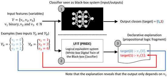
Figure 1. Architecture of the proposed approach for generating an explanation of a given black-box classifier (1) using PRIDE (2) with a toy example (3). Note that the resulting explanations generated by PRIDE are in propositional logic.

The main contributions of this work are:

• We have proposed a method to provide declarative explanations and descriptions using PRIDE of typical machine learning scenarios. Our approach guarantees a logical equivalent version to explain how the outputs are related with the inputs in a general machine learning setup.
• We have applied our proposal to two different domains to check the generality of our approach.

  –

  A multimodal machine learning test-bed around automatic recruitment including different biases (by gender and ethnicity) on synthetic datasets.

  –

  A real dataset about adult incomes taken from US census whose possible biases to get higher earnings are found and shown.

A preliminary version of this article was published in [22]. This new work significantly improves [22] in the following ways:

• We have updated the state of the art methods applicable to XAI.
• We have enriched the introduction to LFIT with examples for a more general audience.
• We have checked the expressiveness of our approach (based on LFIT) extending it to a dataset about adult income level from the 1994 US census. In this domain, we have not used any deep learning algorithms to compare, showing that the proposed approach is also applicable under this circumstance.

The rest of the paper is structured as follows: Section 2 summarises the related relevant literature. Section 3 describes our methodology including LFIT, GULA, and PRIDE. Section 4 presents the experimental framework, including the datasets and experiments conducted. Section 5 presents our results. Finally Section 6 and Section 7 respectively discuss our work and describe our conclusions and further research lines.

2. Related Works

2.1. Explainable AI (XAI): Declarative Approaches

Among the methods suitable to generate explanations because they could be considered as strong or ultra-strong, we find the state of the art evolutionary approaches (from initial genetic programming [23] to grammatical-based methods [24,25,26] and other algebraic ways to express algorithms as straight-line programs [27]); declarative-numeric hybrid (in some way) approaches such as $\delta$ ILP [28] (that mix neural and logic domains) or DeepProbLog [29] (that follows a probabilistic and logic approach); and finally declarative approaches, like the one developed in the present paper.

The state of the art method shows that most of the reviews on XAI identify different methods to explain or interpret black-box machine learning algorithms without considering declarative approaches. Especially noteworthy are the exhaustive treatment of rule extracting systems and the exclusion of formal logic-based methods [30,31,32,33,34], like the one presented here.

In general, the most exhaustive reviews mainly focus on numeric approaches to generate explanations, both for specific domains such as graph neural networks (see [35] and in general [15,36,37]).

We attempt to deeper explain the relationship among LFIT and machine learning algorithms focused on rule sets (including fuzzy logic ones) and decision trees because their outputs syntactically look similar.

In [15], we find a detailed taxonomy that includes these systems. It is clear that they are mostly used in a post-hoc way (explaining the result of a black-box algorithm after being generated) in approaches named explanations by simplification and, in some cases, local explanations.

In the case of local explanations, a set of explanations is generated from the different smaller subsystems that are identified in the global system. It is clear that both (explanation by simplification and local explanations) need to simplify the model that explain, avoiding the complexity of explaining the complete model as a whole. As we have explained before, our research is not interested in approaches that need to simplify the model to generate explanations.

In addition, these approaches are usually supported by numerical engines. Most are driven by the gradient of a loss or gain function. This is not the case with LFIT and other declarative approaches. As we have previously explained, the current research is not interested in these kinds of numerical/statistical approaches.

New possible classifications arise when the declarative dimension is taken into account. If rule sets (generated as outputs) are considered declarative, approaches such as rule-based learners (including fuzzy) and decision trees could be considered hybrids. If each approach is classified by taking into account only the nature of its learning engine, these systems should be considered as numerical/statistical. The authors of the current contribution have previously published an internal report that extends taxonomies like [15] from this viewpoint.

Numerical (statistical) and declarative approaches such as those mentioned in this paper are classical alternatives for facing machine learning. As we have previously explained, they differ in several important features that we can summarise in the following way:

• Statistical approaches need huge amounts of data to extract valid knowledge, while declarative ones are usually able to minimise the set of examples and counterexamples to get the same.
• Statistical approaches are usually compatible with noisy and poorly labelled data, while for declarative ones, this is a circumstance difficult to overcome.
• Statistical approaches do not offer, in the general case, clear explanations about the decisions they make (usually considered as weak machine learning algorithms), while declarative approaches (due to the declarative nature of the formal models that support them) are designed to be at least strong.
• Declarative approaches are supported by formal models like functional programming or formal logic. The theoretical properties of these models make it possible that the learned knowledge exhibits some characteristics (such as logical equivalence, minimisation, etc.)
• Hybrid approaches try to take advantage of both possibilities. Hybridisation can mix a declarative learning engine with numerical components or the opposite. The characteristics of the learned model depend on the type of hybridisation: equivalent noise-tolerant versions of the observed data can be learned by logical engines with numerical input components, and quasi-equivalent logical theories can be approximately induced by numerical/statistical machine learning algorithms that implement differentiable versions of logical operators and inference rules.

2.2. Inductive Programming for XAI

Some meta-heuristic approaches (the aforementioned evolutionary methods) have been used to automatically generate programs. Genetic programming (GP) was introduced by Koza [38] for automatically generating LISP expressions for given tasks expressed as pairs (input/output). This is, in fact, a typical machine learning scenario. GP was extended by the use of formal grammar to generate programs in any arbitrary language, keeping not only syntactic correctness [24] but also semantic properties [26]. Algorithms expressed in any language are declarative versions of the concepts learnt, which makes evolutionary automatic programming algorithms machine learners with good explainability.

Declarative programming paradigms (functional, logical) are as old as computer science and are implemented in multiple ways, e.g., LISP [39], Prolog [40], Datalog [41], Haskell [42], and Answer Set Programs (ASP) [43].

Of particular interest for us within declarative paradigms is logic programming, and in particular, first-order logic programming, which is based on the Robinson’s resolution inference rule that automates the reasoning process of deducing new clauses from a first-order theory [44]. Introducing examples and counter examples and combining this scheme with the ability to extend the initial theory with new clauses, it is possible to automatically induce a new theory that (logically) entails all of the positive examples but none of the negative examples. The underlying theory from which the new one emerges is considered background knowledge. This is the hypothesis of inductive logic programming (ILP [18,45]) that has received a great research effort in the last two decades. Recently, these approaches have been extended to make them noise-tolerant (in order to overcome one of the main drawbacks of ILP vs. statistical/numerical approaches when facing bad-labelled or noisy examples [20]).

Other declarative paradigms are also compatible with ILP, e.g., MagicHaskeller [46], with the functional programming language Haskell; and ILASP [47] for inductively learning answer set programs.

It has been previously mentioned that ILP implies some kind of search in spaces that can become huge. This search can be eased by hybridising with other techniques, e.g., [48] introduces GA-Progol that applies evolutive techniques.

Within ILP methods, we have identified LFIT as especially relevant for explainable AI (XAI). Although LFIT learns propositional logic theories instead of first-order logic, the aforementioned ideas about ILP are still valid. In the next section, we will describe the fundamentals of LFIT and its PRIDE implementation, which will be tested experimentally for XAI in the experiments that will follow.

2.3. Learning from Interpretation Transition (LFIT)

Learning from interpretation transition (LFIT) [49] has been proposed to automatically construct a model of the dynamics of a system from the observation of its state transitions. Given some raw data, like time-series data of gene expression, a discretisation of those data in the form of state transitions is assumed. From those state transitions, according to the semantics of the system dynamics, several inference algorithms modelling the system as a logic program have been proposed. The semantics of a system’s dynamics can indeed differ with regard to the synchronism of its variables, the determinism of its evolution and the influence of its history.

The LFIT framework proposes several modelling and learning algorithms to tackle those different semantics. To date, the following systems have been tackled: memory-less deterministic systems [49], systems with memory [50], probabilistic systems [51], and their multi-valued extensions [52,53]. The work [54], proposes a method that deals with continuous time series data, the abstraction itself being learned by the algorithm.

In [55,56], LFIT was extended to learn system dynamics independently of its update semantics. That extension relies on a modeling of discrete memory-less multi-valued systems as logic programs in which each rule represents a variable that takes some value at the next state, extending the formalism introduced in [49,57]. The representation in [55,56] is based on annotated logics [58,59]. Here, each variable corresponds to a domain of discrete values. In a rule, a literal is an atom annotated with one of these values. It represents annotated atoms simply as classical atoms, and thus, remains at a propositional level. This modelling characterises optimal programs independently of the update semantics. It allows modelling the dynamics of a wide range of discrete systems, including our domain of interest in this paper. LFIT can be used to learn an equivalent propositional logic program that provides explanations for each given observation.

3. Methods

3.1. General Methodology

Figure 2 graphically describes our proposed approach to generate explanations using LFIT of a given black-box classifier. We can see that our purpose is to get declarative explanations in parallel (in a kind of white-blox digital twin) to a given neural network classifier. In the present work, for our first set of experiments, we used the same neural network and datasets described in [8], excluding the face images as explained in the following sections. In our second set of experiments (income prediction) we did not consider any machine learning algorithms to compare with. Therefore, the black box of Figure 2 is not considered in that case, although the rest of the figure is still applicable. In that set of experiments, we explore declarative explanations of the input/output relation of the training/testing datasets.

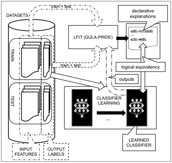
Figure 2. Experimental framework: PRIDE is fed with all the data available (train + test) for increasing the accuracy of the equivalence. In our experiments we consider the classifier (see [8] for details) as a black box to perform regression from input resume attributes (atts.) to output labels (recruitment scores labelled by human resources experts). LFIT gets a digital twin to the neural network providing explainability (as human-readable white-box rules) to the neural network classifier.

3.2. PRIDE Implementation of LFIT

GULA [55,56] and PRIDE [60] are particular implementations of the LFIT framework [49]. In the present section we introduce and describe, first informally and then formally, the notation and the fundamentals of both methods.

Table 1 summarises the dataset about incomes of adults in USA. It shows the names, meaning, type of data, and codification used in our experiments. In the following points we will explain by means of examples over that table the relevant LFIT concepts.

Table 1. Names, values and codification of the dataset about incomes. Attributes of type C take integer or real continuous values and they are uniformly discretised. Attributes of type D are originally discrete and are numerically coded from 0 to the maximum needed value.

Attribute	Meaning	Type	Codification
Age	Age of the individual (years)	C	$\{0,1,\dots ,7\}$
Workclass	Work type (self employment, private, …)	D	$\{0,1,\dots ,6\}$
Fnlwgt	Demographic weight (row) from census	D	$\{0,1,\dots ,14\}$
Education	Highest academic degree	D	$\{0,1,\dots ,15\}$
Marital status	Civil status	D	$\{0,1,\dots ,3\}$
Occupation	Individual’s job sector	D	$\{0,1,\dots ,13\}$
Relationship	Present individual’s relationship	D	$\{0,1,\dots ,5\}$
Ethnicity	Ethnic group	D	$\{0,1,\dots ,4\}$
Sex		D	$\{0,1\}$
Capital gain	Increase in individual’s capital asset	C	$\{0,1,\dots ,9\}$
Capital loss	Decrease in individual’s capital asset	C	$\{0,1,\dots ,4\}$
Hours per week	Spent on work (average)	D	$\{0,1,\dots ,9\}$
Native country	Country of origin	D	$\{0,1,\dots ,40\}$
Income level	Individual’s class of income (≤50, >50)	D	$\{0,1\}$

3.2.1. Multi-Valued Logic

Table 1 shows multi-valued attributes instead of binary. LFIT translates them into propositional ones (binary) creating as many propositional (binary) variables as possible values for each attribute. Although we keep the typical functional notation $var\left(value\right)$, each combination is in fact the propositional variable $va{r}^{value}$.

So, for example, from Table 1, we can have $ag{e}^3$, $educatio{n}^6$, $marital\_statu{s}^0$ or $occupatio{n}^0$ (where the superindexes denote possible data values), which will be actually written as $age\left(3\right)$, $education\left(6\right)$, $marital\_status\left(0\right)$, and $occupation\left(0\right)$.

3.2.2. Rules

LFIT expresses the theory it learns as a set of propositional Horn clauses with exactly one positive literal, that is, as logical implications between a conjunction of propositional atoms in the following form:

$$h^{va{l}_h^i}\leftarrow p_1^{va{l}_1^{i_1}}\wedge \dots \wedge p_n^{va{l}_n^{i_n}}$$

(1)

The Prolog form shown in Listing 1 is usually preferred.

Listing 1. Prolog notation for LFIT rules.

$h\left(va{l}_h^i\right)$ :- $p_1\left(va{l}_1^{i_1}\right)$ ,…, $p_n\left(va{l}_n^{i_n}\right)$.

Listing 1. Prolog notation for LFIT rules.

$h\left(va{l}_h^i\right)$ :- $p_1\left(va{l}_1^{i_1}\right)$ ,…, $p_n\left(va{l}_n^{i_n}\right)$.

In the domain of adult incomes we could find rules like those shown in Listing 2.

Listing 2. Prolog version of rules learnt by LFIT in the case study related to Table 1.

class(0) :- age(3), education(6), marital-status(0), occupation(0).

class(0) :- age(4), workclass(0), education(1), occupation(8), relationship(0), native-country(0).

class(1) :- education(7), marital-status(5).

class(1) :- age(2), education(8), occupation(10).

class(1) :- age(1), education(3), marital-status(2), occupation(9).

Listing 2. Prolog version of rules learnt by LFIT in the case study related to Table 1.

class(0) :- age(3), education(6), marital-status(0), occupation(0).

class(0) :- age(4), workclass(0), education(1), occupation(8), relationship(0), native-country(0).

class(1) :- education(7), marital-status(5).

class(1) :- age(2), education(8), occupation(10).

class(1) :- age(1), education(3), marital-status(2), occupation(9).

3.2.3. Rule Domination

In the LFIT learning process, rule domination is an important concept. Roughly speaking, when they have the same head, a rule dominates another if its body is contained in the others.

In Listing 3 you can see how $R_1$ dominates $R_2$.

Listing 3. Example of rule domination.

$R_1$: class(0) :- education(6), marital-status(0).

$R_2$: class(0) :- age(3), education(6), marital-status(0), occupation(0).

Listing 3. Example of rule domination.

$R_1$: class(0) :- education(6), marital-status(0).

$R_2$: class(0) :- age(3), education(6), marital-status(0), occupation(0).

Dominant rules can be considered more general and are the goal of LFIT.

3.2.4. States and Rule-State Matching

Rule generation in LFIT starts from the design of a body that fits as many examples as possible. This is done by rule-state matching. Informally, a state is a conjunction of atoms (positive literals, that is, associations between attributes and specific values) that could describe one or more examples.

A rule and a state match if the body of the rule is included in the state.

Listing 4 shows an example of rule-state matching: state $s_1$ and rule $R_1$ does.

Listing 4. Example of rule-state matching.

$s_1$: age(3), education(6), marital-status(0), occupation(0)

$R_1$: class(0) :- education(6), marital-status(0).

Listing 4. Example of rule-state matching.

$s_1$: age(3), education(6), marital-status(0), occupation(0)

$R_1$: class(0) :- education(6), marital-status(0).

In the following, we denote by $\mathbb{N}:=\{0,1,2,\dots \}$, the set of natural numbers, and for all $k,n\in \mathbb{N}$, $〚k;n〛:=\{i\in \mathbb{N}\mid k\le i\le n\}$ is the set of natural numbers between k and n included. For any set S, the cardinal of S is denoted $\left|S\right|$ and the power set of S is denoted $\wp \left(S\right)$.

Let $\mathcal{V}=\{{\mathrm{v}}_1,\dots ,{\mathrm{v}}_n\}$ be a finite set of $n\in \mathbb{N}$ variables, $\mathcal{V}al$ the set in which variables take their values and $\mathsf{dom}:\mathcal{V}\to \wp \left(\mathcal{V}al\right)$ a function associating a domain to each variable. The atoms of $\mathcal{M}\mathrm{V}\mathrm{L}$ (multi-valued logic) are of the form ${\mathrm{v}}^{val}$ where $\mathrm{v}\in \mathcal{V}$ and $val\in \mathsf{dom}\left(\mathrm{v}\right)$. The set of such atoms is denoted by ${\mathcal{A}}_{\mathsf{dom}}^{\mathcal{V}}=\{{\mathrm{v}}^{val}\in \mathcal{V}\times \mathcal{V}al\mid val\in \mathsf{dom}\left(\mathrm{v}\right)\}$ for a given set of variables $\mathcal{V}$ and a given domain function $\mathsf{dom}$. In the following, we work on specific $\mathcal{V}$ and $\mathsf{dom}$ that we omit to mention when the context makes no ambiguity, thus simply writing $\mathcal{A}$ for ${\mathcal{A}}_{\mathsf{dom}}^{\mathcal{V}}$.

Example 1.

For a system of three variables, the typical set of variables is $\mathcal{V}=\{a,b,c\}$. In general, $\mathcal{V}al=\mathbb{N}$ so that domains are sets of natural integers, for instance: $\mathsf{dom}\left(a\right)=\{0,1\}$, $\mathsf{dom}\left(b\right)=\{0,1,2\}$ and $\mathsf{dom}\left(c\right)=\{0,1,2,3\}$. Thus, the set of all atoms is: $\mathcal{A}=\{a^0,a^1,b^0,b^1,b^2,c^0,c^1,c^2,c^3\}$.

An $\mathcal{M}\mathrm{V}\mathrm{L}$ rule R is defined by:

$$R={\mathrm{v}}_0^{{val}_0}\leftarrow {\mathrm{v}}_1^{{val}_1}\wedge \dots \wedge {\mathrm{v}}_m^{{val}_m}$$

(2)

where $\forall i\in 〚0;m〛,{\mathrm{v}}_i^{{val}_i}\in \mathcal{A}$ are atoms in $\mathcal{M}\mathrm{V}\mathrm{L}$ so that every variable is mentioned at most once in the right-hand part: $\forall j,k\in 〚1;m〛,j\ne k\Rightarrow {\mathrm{v}}_j\ne {\mathrm{v}}_k$. Intuitively, the rule R has the following meaning: the variable ${\mathrm{v}}_0$ can take the value ${val}_0$ in the next dynamical step if for each $i\in 〚1;m〛$, variable ${\mathrm{v}}_i$ has value ${val}_i$ in the current dynamical step.

The atom on the left-hand side of the arrow is called the head of R and is denoted $h\left(R\right):={\mathrm{v}}_0^{{val}_0}$. The notation $\mathrm{var}\left(h\left(R\right)\right):={\mathrm{v}}_0$ denotes the variable that occurs in $h\left(R\right)$. The conjunction on the right-hand side of the arrow is called the body of R, written $b\left(R\right)$ and can be assimilated to the set $\{{\mathrm{v}}_1^{{val}_1},\dots ,{\mathrm{v}}_m^{{val}_m}\}$; we thus use set operations such as ∈ and ∩ on it. The notation $\mathrm{var}\left(b\left(R\right)\right):=\{{\mathrm{v}}_1,\dots ,{\mathrm{v}}_m\}$ denotes the set of variables that occurs in $b\left(R\right)$. More generally, for all set of atoms $X\subseteq \mathcal{A}$, we denote $\mathrm{var}\left(X\right):=\{\mathrm{v}\in \mathcal{V}\mid \exists val\in \mathsf{dom}\left(\mathrm{v}\right),{\mathrm{v}}^{val}\in X\}$ the set of variables appearing in the atoms of X. A multi-valued logic program ($\mathcal{M}\mathrm{V}\mathrm{L}\mathrm{P}$) is a set of $\mathcal{M}\mathrm{V}\mathrm{L}$ rules.

Definition 1 introduces a domination relation between rules that defines a partial anti-symmetric ordering. Rules with the most general bodies dominate the other rules. In practice, these are the rules we are interested in since they cover the most general cases.

Definition 1

(Rule Domination). Let $R_1$, $R_2$ be two $\mathcal{M}\mathrm{V}\mathrm{L}$ rules. The rule $R_1$ dominates $R_2$, written $R_2\le R_1$ if $h\left(R_1\right)=h\left(R_2\right)$ and $b\left(R_1\right)\subseteq b\left(R_2\right)$.

In [56], the set of variables is divided into two disjoint subsets: $\mathcal{T}$ (for targets) and $\mathcal{F}$ (for features). This allows us to define a dynamic $\mathcal{M}\mathrm{V}\mathrm{L}\mathrm{P}$, which captures the dynamics of the problems we tackle in this paper.

Definition 2

(Dynamic $\mathcal{M}\mathrm{V}\mathrm{L}\mathrm{P}$). Let $\mathcal{T}\subset \mathcal{V}$ and $\mathcal{F}\subset \mathcal{V}$ such that $\mathcal{F}=\mathcal{V}\setminus \mathcal{T}$. A $\mathcal{D}\mathcal{M}\mathrm{V}\mathrm{L}\mathrm{P}$ P is a $\mathcal{M}\mathrm{V}\mathrm{L}\mathrm{P}$ such that $\forall R\in P,\mathrm{var}\left(h\left(R\right)\right)\in \mathcal{T}$ and $\forall {\mathrm{v}}^{val}\in b\left(R\right),\mathrm{v}\in \mathcal{F}$.

The dynamical system we want to learn the rules of is represented by a succession of states as formally given by Definition 3. We also define the “compatibility” of a rule with a state in Definition 4.

Definition 3

(Discrete state). A discrete state s on $\mathcal{T}$ (resp. $\mathcal{F}$) of a $\mathcal{D}\mathcal{M}\mathrm{V}\mathrm{L}\mathrm{P}$ is a function from $\mathcal{T}$ (resp. $\mathcal{F}$) to $\mathbb{N}$, i.e., it associates an integer value to each variable in $\mathcal{T}$ (resp. $\mathcal{F}$). It can be equivalently represented by the set of atoms $\{{\mathrm{v}}^{s\left(\mathrm{v}\right)}\mid \mathrm{v}\in \mathcal{T}(resp.\mathcal{F})\}$ and thus we can use classical set operations on it. We write ${\mathcal{S}}^{\mathcal{T}}$ (resp. ${\mathcal{S}}^{\mathcal{F}}$) to denote the set of all discrete states of $\mathcal{T}$ (resp. $\mathcal{F}$), and a couple of states$(s,s^{\prime })\in {\mathcal{S}}^{\mathcal{F}}\times {\mathcal{S}}^{\mathcal{T}}$ is called a transition.

Definition 4

(Rule-state matching). Let $s\in {\mathcal{S}}^{\mathcal{F}}$. The $\mathcal{M}\mathrm{V}\mathrm{L}$ rule R matches s, written $R\sqcap s$, if $b\left(R\right)\subseteq s$.

The notion of transition in LFIT corresponds to a data sample in the problems we tackle in this paper: a couple of input features and a target label. When a rule matches a state, it can be considered as a possible explanation to the corresponding observation. The final program we want to learn should both:

• Match the observations in a complete (all observations are explained) and correct (no spurious explanation) way;
• Represent only minimally necessary interactions (according to Occam’s razor: no overly-complex bodies of rules).

GULA [55,56] and PRIDE [60] can produce such programs.

Formally, given a set of observations T, GULA [55,56] and PRIDE [60] will learn a set of rules P such that all observations are explained: $\forall (s,s^{\prime })\in T,\forall {\mathrm{v}}^{val}\in s^{\prime },\exists R\in P,R\sqcap s,h\left(R\right)={\mathrm{v}}^{val}$. All rules of P are correct w.r.t. T: $\forall R\in P,\forall (s1,s2)\in T,R\sqcap s1\Rightarrow \exists (s1,s3)\in T,h\left(R\right)\in s3$ (if T is deterministic, $s2=s3$). All rules are minimal w.r.t. $\mathcal{F}$: $\forall R\in P,\forall R^{\prime }\in \mathcal{M}\mathrm{V}\mathrm{L}\mathrm{P},R^{\prime }$ correct w.r.t. T it holds that $R\le R^{\prime }\Rightarrow R^{\prime }=R$.

The possible explanations of an observation are the rules that match the feature state of this observation. The body of rules gives a minimal condition over feature variables to obtain its conclusions over a target variable. Multiple rules can match the same feature state, thus multiple explanations can be possible. Rules can be weighted by the number of observations they match to assert their level of confidence. Output programs of GULA and PRIDE can also be used in order to predict and explain from unseen feature states by learning additional rules that encode when a target variable value is not possible as shown in the experiments of [56].

The current contribution shows a possible application of a declarative method (such as LFIT) in some scenarios with numerical aspects: in the FairCV db case we are generating white-box explanations to a deep-learner black-box; in the US census case we are explaining a dataset that could be typically tackled by numeric (statistical) approaches.

In these situations there is an interesting question regarding qualitative vs. quantitative considerations.

From the declarative viewpoint of LFIT, the focus is on the qualitative guarantee of learning a logical version equivalent to the observed system. Regarding equivalence, the version is equivalent or it is not. If the model fails in 1% of the examples, equivalence is lost in the same way than if it had failed in 20% or 60% of the examples.

From the viewpoint of the statistical approaches it is very important to take into account the amounts. For example, the output of deep-learning classifiers is based on a quantitative criterion such as to choose the label with the highest probability.

It could seem that the qualitative behaviour of LFIT does not matter; but this is not exactly true.

LFIT can easily collect qualitative information, such as how many states (input examples) match each rule. This numerical information can be used as weights, both to better explain and understand the process, but also to incorporate predicting capabilities to the declarative version. This option has been explained and explored in [61,62].

4. Experimental Framework

For testing the capability of PRIDE to explain machine learning domains we have designed several experiments using the FairCVdb dataset [8] and the data about adult incomes from the 1994 US census [63].

Although the goals and methods are similar, there are big differences between the tasks. The detailed process is described separately.

4.1. FairCVdb Dataset

FairCVdb comprises 24,000 synthetic resume profiles. Table 2 summarises the structure of these data. Each resume includes 12 features (${\mathrm{v}}_i$) related to the candidate merits, 2 demographic attributes (gender and three ethnicity groups), and a face photograph. In our experiments we discarded the face image for simplicity (unstructured image data will be explored in future work). Each of the profiles includes three target scores (T) generated as a linear combination of the 12 features:

$$T=\beta +\sum _{i=1}^{12}{\alpha }_i·{\mathrm{v}}_i,$$

(3)

where ${\alpha }_i$ is a weighting factor for each of the merits (see [8] for details): $\left(i\right)$ unbiased score ($\beta =0$); $\left(ii\right)$ gender-biased scores ($\beta =0.2$ for male and $\beta =0$ for female candidates); and $\left(iii\right)$ ethnicity-biased scores ($\beta =0.0,0.15$ and $0.3$ for candidates from ethnic groups 1, 2, and 3, respectively). Thus, we intentionally introduce bias into the candidate scores. From this point on, we will simplify the name of the attributes considering g for gender, e for ethnic group, and $i1$ to $i12$ for the rest of the input attributes. In addition to the bias previously introduced, some other random bias was introduced relating attributes and gender to simulate real social dynamics. The attributes concerned were $i3$ and $i7$. Note that merits were generated without bias, assuming an ideal scenario where candidate competencies do not depend on their gender or ethnic group. For the current work we have used only discrete values for each attribute discretising one attribute (experience to take values from 0 to 5, the higher the better) and the scores (from 0 to 3) that were real valued in [8].

Table 2. Names, values, and codification of the FairCVdb dataset. Attributes of type C take continuous real values and are uniformly discretised. Attributes of type D are discrete and are numerically coded from 0 to the maximum needed value. For all values the higher is considered the better.

Attribute	Meaning	Type	Codification
Ethnicity	Ethnic group	D	$\{0,1,2\}$
Gender		D	$\{0,1\}$
Education	Education level	D	$\{0,1,\dots ,5\}$
Experience	Work experience	C	$\{0,1,\dots ,4\}$
Availability	Time for being ready to start	D	$\{0,1,\dots ,5\}$
Foreign languages	Level of 8 possible languages	D	$\{0,1,\dots ,3\}$
Score	Unbiased value assigned	C	$\{0,1,\dots ,3\}$
Gender biased score	(Gender) biased value assigned	C	$\{0,1,\dots ,3\}$
Ethnicity biased score	(Ethnicity) biased value assigned	C	$\{0,1,\dots ,3\}$

Experimental Protocol: Towards Declarative Explanations

We have experimented with PRIDE on the FairCVdb dataset described in the previous section.

Figure 3 shows names and explains the scenarios considered in our experiments. In [8], researchers demonstrate that an automatic recruitment algorithm based on multimodal machine learning reproduces existing biases in the target functions even if demographic information was not available as input (see [8] for details). Our purpose in the experiments was to obtain a declarative explanation capable of revealing those biases.

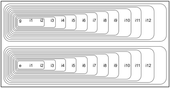
Figure 3. Structure of the experimental tests. There are 4 datasets for analysing gender (named g) and ethnicity (e) bias separately. Apart from gender and ethnicity, there are 12 other input attributes (named from $i1$ to $i12$). There is a couple of (biased and unbiased) datasets for each one: gender and ethnicity. We have studied the input attributes by increasing complexity starting with $i1$ and $i2$ and adding one at each time. Thus, for each couple we considered 11 different scenarios (named from $s1$ to $s11$). This figure shows their structure ($s_i$ is included in all $s_j$ for which $i<j$).

4.2. Adult Income Level Dataset

In a second set of experiments, we considered a dataset about adult incomes extracted from the 1994 US census [63]. It contains a total of 48,842 entries with 14 attributes that describe the group of individuals represented by each entry. One of these attributes is the income level discretised to only highlight if it is high (>50 k USD) or low (≤50 k USD). Table 1 summarises the structure of the dataset.

The dataset is usually split into training and testing subsets. Like in the first analysis on the FairCVdb dataset, we fed PRIDE with the complete dataset.

Unlike the first set of experiments on FairCVdb, with the adult income dataset there was no guarantee that incomes are biased by attributes like gender or ethnicity. Another difference is that datasets taken from the US census are not synthetic; they collect information about real people. In addition, an unbiased version of the income level is not available. On the other hand, there is a common belief that the level of income is skewed by gender and ethnicity. The general intuition tells us that males are more likely to have higher incomes than females, and people of white ethnicity are more likely to have higher incomes than other ethnicities. The goal of this second set of experiments over the income dataset was to check PRIDE expressiveness when trying to find a data-driven explanation for this common belief.

Experiments Design

We followed these steps:

• To prepare the dataset for PRIDE by preprocessing:
  • Removing those entries with some unknown attribute. Only 45,222 entries remain after this step.
  • Discretising continuous attributes (those marked as continuous in Table 1).
• To get a logical version equivalent to the data to analyse the effect of the attribute sex considering the income level as a function of the other attributes.
• To get a logical version equivalent to the data to analyse the effect of the attribute ethnicity considering the income level as a function of the other attributes.

5. Results

It is important to pay attention to the properties that the formal model under LFIT guarantees: the learned propositional logic theory is equivalent to the observed data, and the conditions of each clause (rule) are minimal. These properties allow for estimating the complexity of the observed data from the complexity of the learned theory—the simpler the dataset the simpler the theories. In the future, we would like to explore the possibility of defining some kind of complexity measure of the datasets from the complexity of the theories learned by LFIT. It could be something similar to Kolmogorov’s compression complexity [64].

Another important question to take into account when quantitatively analysing these results is the expressiveness of the LFIT models. Propositional logic excludes the use of variables. Although functional notation has been used (for example in $sex\left(0\right)$) each pair of functions and one specific value of its argument, represents a proposition ($se{x}^0$ in our example). The use of variables by other declarative models, such as first-order logic, allows a more compact notation by grouping different values of the same attribute by means of a well defined variable. However, there is no trivial translation from one model to another. It is important to realise that this circumstance is an inherent characteristic of propositional logic that can not be overcome inside the propositional realm. It is true that more compact notations could be more readable and, hence, they can offer more easily understandable explanations. However, the increase of the readability of LFIT results by translating them into another model is out of the scope of the current contribution.

5.1. FairCVdb Dataset

5.1.1. Example of Declarative Explanation

Listing 5 shows a fragment generated with the proposed methods for scenario $s1$ for gender-biased scores. We have chosen a fragment that fully explains how a CV is scored with the value three for Scenario 1. Scenario 1 takes into account the input attributes gender, education, and experience. The first clause (rule), for example, says that if the value of a CV for the attribute gender is 1 (female), for education is 5 (the highest), and for experience is 3, then this CV receives the highest score (3).

The resulting explanation is a propositional logic fragment equivalent to the classifier for the data. It can also be understood as a set of rules with the same behavior. From the viewpoint of explainable AI, this resulting fragment can be understood by an expert in the domain and used to generate new knowledge about the scoring of CVs.

Listing 5. Fragment of explanation for scoring 3.

scores(3) :- gender(1), education(5), experience(3).

scores(3) :- education(4), experience(3).

Listing 5. Fragment of explanation for scoring 3.

scores(3) :- gender(1), education(5), experience(3).

scores(3) :- education(4), experience(3).

5.1.2. Quantitative Summary of the Results

In this section, a quantitative summary of the results is discussed. The total number of rules and the frequency of each attribute are shown. In order to compare the influence of each attribute, their normalised frequencies with respect to the total number of rules are also shown.

Table 3 and Table 4 show the number of rules and the absolute frequency of each attribute in the rules when comparing ethnicity biased and unbiased datasets.

Table 3. Frequency of the first attributes when explaining ethnicity biases.

	e	i1	i2	i3	i4	i5	i6
Ethnic bias	3221	3648	2802	1789	2951	3300	1520
No ethnic bias	1682	2398	1822	1065	1846	2032	1023

Table 4. Frequency of the last attributes when explaining ethnicity biases.

	i7	i8	i9	i10	i11	i12	#Rules
Ethnic bias	1449	1404	1214	1044	870	652	7886
No ethnic bias	892	875	805	683	544	397	2732

Table 5 and Table 6 show the number of rules and the absolute frequency of each attribute in the rules when comparing gender biased and unbiased datasets.

Table 5. Frequency of the first attributes when explaining gender biases.

	g	i1	i2	i3	i4	i5	i6
Gender bias	1150	2164	1671	1006	1642	1830	884
No gender bias	992	1943	1524	861	1445	1663	832

Table 6. Frequency of the last attributes when explaining gender biases.

	i7	i8	i9	i10	i11	i12	#Rules
Gender bias	874	807	681	630	537	347	2449
No gender bias	714	714	633	557	470	320	2200

In order to compare the effect of each attribute, their normalised frequencies (with respect to the number of rules) are also shown in Figure 4 (when studying ethnicity biases) and in Figure 5 (for gender biases).

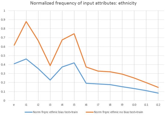
Figure 4. Normalised frequency of attributes when studying ethnic biases.

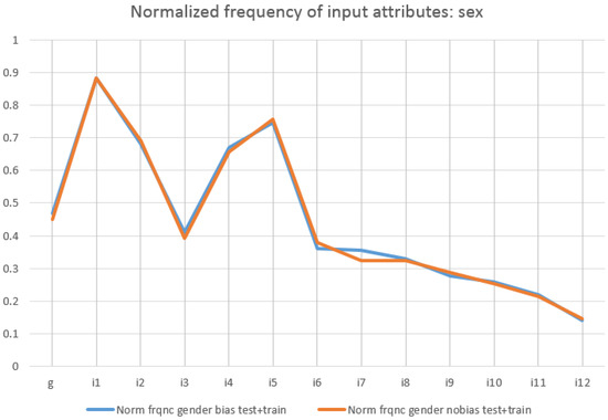
Figure 5. Normalised frequency of attributes when studying gender biases.

5.1.3. Quantitative Identification of Biased Attributes in Rules

Our quantitative results are divided in two parts. The first part is based on the fact that, in the biased experiments, if $gender\left(0\right)$ appears more frequently than $gender\left(1\right)$ in the rules, then that would lead to higher scores for $gender\left(0\right)$. In the second quantitative experimental part we will show the influence of bias in the distribution of attributes.

We first define Partial Weight $PW$ as follows. For any program P and two atoms $v_0^{va{l}_0^i}$ and $v_1^{va{l}_1^j}$, where $va{l}_0^i\in va{l}_0$ and $va{l}_1^i\in va{l}_1$, define:

$$S=\{R|R\in P\wedge v_0^{va{l}_0^i}\in h\left(R\right)\wedge v_1^{va{l}_1^j}\in b\left(R\right)\}$$

.

Then we have: $P{W}_{v_1^{va{l}_1^j}}\left(v_0^{va{l}_0^0}\right)=\left|S\right|$. A more accurate $PW$ could be defined, for example, by setting different weights for rules with different lengths. For our purpose, the frequency is enough. In our analysis, the number of examples for compared scenarios are consistent.

Depending on $PW$, we define global weight $GW$ as follows. For any program P and $v_1^{va{l}_1^j}$, we have: $G{W}_{v_1^{va{l}_1^j}}={\sum }_{va{l}_0^i\in va{l}_0}P{W}_{v_1^{va{l}_1^j}}\left(v_0^{va{l}_0^i}\right)·va{l}_0^i$. The $G{W}_{v_1^{va{l}_1^j}}$ is a weighted addition of all the values of the output, and the weight, in our case, is the value of scores.

This analysis was performed only on scenario $s11$, comparing unbiased and gender- and ethnicity-biased scores. We have observed a similar behavior of both parameters: partial and global weights. In unbiased scenarios, the distributions of the occurrences of each value could be considered statistically the same (between gender(0) and gender(1) and among ethnicity(0), ethnicity(1) and ethnicity(2)). Nevertheless, in biased datasets the occurrences of gender(0) and ethnic(0) for higher scores are significantly higher. The maximum difference even triplicates the occurrence of the other values.

For the global weights, for example, the maximum differences in the number of occurrences, without and with bias respectively, for higher scores expressed as % increases from $48.8\%$ to $78.1\%$ for gender(0), while for gender(1) decreases from $51.2\%$ to $21.9\%$. In the case of ethnicity, it increases from $33.4\%$ to $65.9\%$ for ethnic(0), but decreases from $33.7\%$ to $19.4\%$ for ethnic(1) and from $32.9\%$ to $14.7\%$ for ethnic(2).

5.1.4. Quantitative Identification of the Distribution of Biased Attributes

We now define $fre{q}_{p_1}\left(a\right)$ as the frequency of attribute a in $P_1$. The normalised percentage for input a is: $N{P}_{p_1}\left(a\right)=fre{q}_{p_1}\left(a\right)/{\sum }_{x\in input}fre{q}_{p_1}\left(x\right)$ and the percentage of the absolute increment for each input from unbiased experiments to its corresponding biased ones is defined as: $AI{P}_{p_1,p_2}\left(a\right)=(fre{q}_{p_1}\left(a\right)-fre{q}_{p_2}\left(a\right))/fre{q}_{p_2}\left(a\right)$.

In this approach we have taken into account all scenarios (from $s1$ to $s11$) for both gender and ethnicity.

We have observed that for both parameters the only attributes that consistently increase their values are gender and ethnicity comparing unbiased and gender/ethnicity-biased scores. Figure 6 and Figure 7 show $AI{P}_{us1-11,ebs1-11}$ for each attribute, that is, their values comparing unbiased and ethnic-biased scores for all scenarios from $s1$ to $s11$. It is clear that the highest values correspond to the attribute ethnicity.

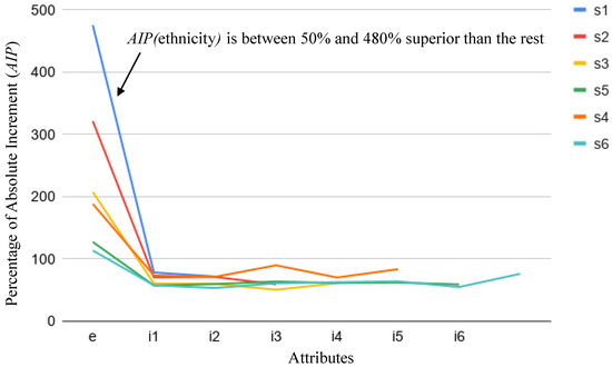
Figure 6. Percentage of the absolute increment (comparing scores with and without bias for ethnicity) of each attribute for scenarios s1, s2, s3, s4, s5 and s6 ($AI{P}_{us1-6,ebs1-6}$). The graphs link the points corresponding to all the input attributes considered in each scenario.

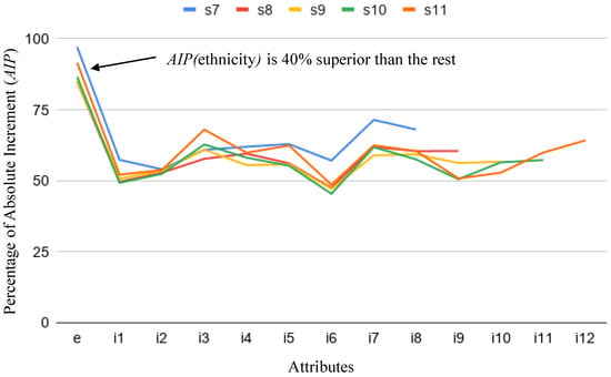
Figure 7. $AI{P}_{us7-11,ebs7-11}$.

Something similar happens for gender. Figure 8 and Figure 9 show $AI{P}_{us1-11,gbs1-11}$ for each attribute when studying gender-biased scores. It is worth mentioning that some differences exist in scenarios $s9$, $s10$, and $s11$, regarding attributes $i3$ and $i7$. These apparent anomalies are explained by the random bias introduced in the datasets in order to relate these attributes with gender when the score is biased. Figure 10 shows $N{P}_{s11}$ for all attributes. This clearly shows the small relevance of attributes $i3$ and $i7$ in the final biased score. As is highlighted elsewhere, this capability of PRIDE to identify random indirect perturbations of other attributes in the bias is a relevant achievement of our proposal.

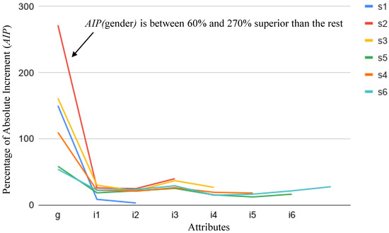
Figure 8. $AI{P}_{us1-6,ebs1-6}$.

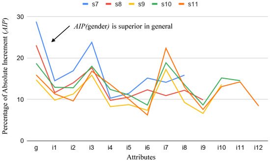
Figure 9. $AI{P}_{us7-11,gbs7-11}$.

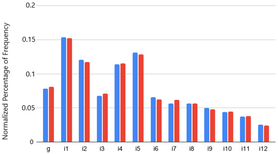
Figure 10. Normalised percentage of frequency in scenario s11 of each attribute: g, i1 to i11 ($N{P}_{s11}$). No bias (blue), gender-biased scores (red).

5.2. Adult Income Level Dataset

A quantitative summary of the dataset can be found in the next paragraphs. Table 7 and Table 8 show the frequency of each attribute when studying ethnicity biases.

Table 7. Frequency of the first attributes when explaining ethnicity bias.

	#Rules	Age	Workclass	Education	ed.#	Civil-Status	Occu.
ethnc.	7948	5478	4612	7007	6902	3737	5860

Table 8. Frequency of the last attributes when explaining ethnicity bias.

	Relationship	Ethnc/Sex	Cap-Gain	Cap-Loss	h/Week	Country
ethnc.	1656	1263	374	813	1605	554

Table 9 and Table 10 show the frequency of each attribute when studying gender biases.

Table 9. Frequency of the first attributes when explaining gender bias.

	#Rules	Age	Workclass	Education	ed.#	Civil-Status	Occu.
gender	7735	5353	4522	6821	6633	3696	5634

Table 10. Frequency of the last attributes when explaining gender biases.

	Relationship	Ethnc/Sex	Cap-Gain	Cap-Loss	h/Week	Country
gender	1620	478	374	832	1685	810

Figure 11 shows the normalised frequency of these attributes. It is easy to check that LFIT catches the structure of the dataset because there are no significative differences when excluding gender or ethnicity to study their biases. It is also interesting to mention that these attributes do not contribute the most to income level.

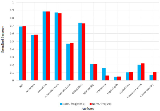
Figure 11. Normalised percentage of frequency in scenario s11 of each attribute: g, i1 to i11 ($N{P}_{s11}$). No bias (blue), gender-biased scores (red).

Due to the circumstances described in previous sections the goals and analysis on this dataset are simpler than on FairCVdb.

In this case, it was enough to study the clauses of the learned program and compute the normalised frequency of the different values of the attributes ethnicity and sex with respect to the total amount of entries and compare the proportion of class(0) and class(1). The results are shown in Figure 12 and Figure 13.

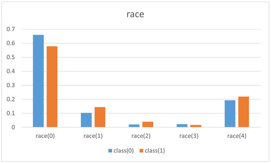
Figure 12. The normalised frequency of different ethnicity and income.

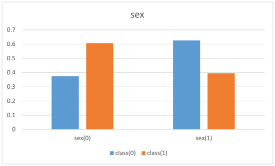
Figure 13. The normalised frequency of different sex and income.

In both cases, blue color is used for class(0) and red for class(1). Their frequency normalised with respect to the total amount of entries are put together to compare them.

This simple initial experiment shows that the propositional logic theory learnt by PRIDE supports and explains the common belief about the relationship among sex (idem. ethnicity) and higher income level:

• Ethnicity: Figure 12 shows that the logical theory contains clauses to explain that people of white ethnicity ethnicity(0) get higher incomes than other ethnicities.
• Sex: Figure 13 shows that the logical theory contains clauses to explain that males sex(1) get higher incomes than females.

Table 11 shows the frequency of values of ethnicity and their effect on income. It is easy to draw the same conclusions explained before. The same happens with respect to gender as Table 12 shows.

Table 11. Frequency of the different values of ethnicity and their effect on income level.

	ethnc(0)	ethnc(1)	ethnc(2)	ethnc(3)	ethnc(4)
class(0)	452	71	14	16	132
class(1)	334	84	23	10	127

Table 12. Frequency of the different values of sex and their effect on income level.

	Sex(0)	Sex(1)
class(0)	101	169
class(1)	126	82

6. Discussion

After running the experiments described in the previous sections we can extract the following conclusions.

• PRIDE canexplainalgorithms learnt by neural networks. The theorems that support the characteristics of PRIDE allow a set of propositional clauses logically equivalent to the systems observed when facing the input data provided. In addition, each proposition has a set of conditions that is minimum. Thus, regarding the FairCVdb case, once the scorer is learnt, PRIDE translates it into a logical equivalent program. This program is a list of clauses like the one shown in Listing 5. Logical programs are declarative theories that explain the knowledge on a domain.
• PRIDE canexplainwhat happens in a specific domain. Our experimental results discover these characteristics of the domain:

  –

  Insights into the structure of the FairCVd dataset. We have seen (and further confirmed with the authors of the datasets) characteristics of the datasets, e.g., (1) All attributes are needed for the score. We have learnt the logical version of the system starting from only two input attributes and including one additional attribute at a time and only reached an accuracy of 100% when taking into account all of them. This is because removing some attributes generates indistinguishable CVs (all the remainder attributes have the same value) with different scores (that correspond to different values in some of the removed attributes). (2) Gender and ethnicity are not the most relevant attributes for scoring: The number of occurrences of these attributes is much smaller than others in the conditions of the clauses of the learnt logical program. (3) While trying to catch the biases we have discovered that some attributes seem to increase their relevance when the score is biased. For example, the competence in some specific languages (attribute i7) seems to be more relevant when the score has gender bias. After discussing with the authors of the datasets, they confirmed a random perturbation of these languages into the biases, that explained our observations.

  –

  Biases in the training FairCVdb datasets were detected. We have analysed the relationship between the scores and the specific values of the attributes used to generate the biased data. We have proposed a simple mathematical model based on the effective weights of the attributes that concludes that higher values of the scores correspond to the same specific values of gender (for gender bias) and ethnic group (for ethnicity bias). On the other hand, we have performed an exhaustive series of experiments to analyse the increase of the presence of the gender and ethnicity in the conditions of the clauses of the learnt logical program (comparing the unbiased and biased versions).

  –

  Insights into the structure of dataset about the adult income from the US census. In this case, there is no unbiased version to compare with, as in the FairCVdb dataset. In addition, we do not have any machine learning approach to be considered for the black-box explanation. Nevertheless, there exists a common belief about the presence of biases (gender and ethnicity) in the income level. PRIDE has been used considering the dataset itself as a black-box, understanding the income level as a function of the other attributes. We have obtained a logic theory that supports this common belief.

Our overall conclusion is that in scenarios in which opaque (black-box) machine learning techniques have been used; LFIT, and in particular PRIDE, are able to offer explanations to the algorithm learnt in the domain under consideration. The resulting explanation is, as well, expressive enough to catch training biases in the models learnt with neural networks.

In those cases in which there is no machine learner to compare with, PRIDE is still able to explain the structure of the datasets considering themselves as the black-box that has to be explained.

7. Further Research Lines

• Increasing understandability. Two possibilities could be considered in the future: (1) to ad hoc post-process the learned program for translating it into a more abstract form, or (2) to increase the expressive power of the formal model that supports the learning engine using, for example, ILP based on first-order logic.
• Adding predictive capability. PRIDE is actually not aimed to predict but to explain (declaratively) by means of a digital twin of the observed systems. Nevertheless, it is not really complicated to extend PRIDE functionality to predict. It should be necessary to change the way in which the result is interpreted as a logical program: mainly by adding mechanisms to chose the most promising rule when more than one is applicable.
  Our plan is to test an extended-to-predict PRIDE version to this same domain and compare the result with the classifier generated by deep learning algorithms.
• Handling numerical inputs. [8] included as input the images of the faces of the owners of the CVs. Although some variants to PRIDE are able to cope with numerical signals, the huge amount of information associated with images implies performance problems. Images are a typical input format in real deep learning domains. We would like to add some automatic pre-processing steps for extracting discrete information (such as semantic labels) from input images. We are motivated by the success of systems with similar approaches but different structure like [65].
• Generating and combining multiple explanations. The present work has explored a way to provide a single human-readable explanation of the behavior of an AI model. An extension we have in mind is generating multiple explanations by different complementary methods and parameters of those methods and then generating a combined explanation [66,67].
• Explaining AI vulnerabilities. Another extension of the presented work is towards explaining unexpected behaviors and vulnerabilites of given AI systems, e.g., against potential attacks [68] like manipulated input data [69].
• Measuring the accuracy and performance of the explanations. As far as the authors know, there is no standard procedure to evaluate and compare different explainability approaches. We will incorporate in future versions some formal metric.
• Analysing other significant problems where non-explainable AI is now the common practice for good explanations. The scenario studied here (automatic tools for screening in recruitment and estimating the income level based on demographic information) are only two of the many application areas where explanations of the action of AI systems are really needed. Other areas that will significantly benefit from this kind of approaches are e-learning [70], e-health [71,72], and other human-computer interaction applications [73,74].
• Proposing metrics for the complexity of the datasets. Due to the formal properties that the general LFIT model gives to the learned theories, the complexity of the original data could be estimated from the complexity of the propositional logic equivalent theory. This approach is inspired by some implementations of Kolmogorov’s complexity by means of file compressors [64].

References

- Senior, A.; Vanhoucke, V.; Nguyen, P.; Sainath, T. Deep neural networks for acoustic modeling in speech recognition. IEEE Signal Process. Mag. 2012, 29, 82–97. [Google Scholar]
- Deng, J.; Dong, W.; Socher, R.; Li, L.J.; Li, K.; Fei-Fei, L. ImageNet: A Large-Scale Hierarchical Image Database. In Proceedings of the 2009 IEEE Conference on Computer Vision and Pattern Recognition, Miami, FL, USA, 20–25 June 2009. [Google Scholar]
- Wu, Y.; Schuster, M.; Chen, Z.; Le, Q.V.; Norouzi, M.; Macherey, W.; Klingner, J. Google’s neural machine translation system: Bridging the gap between human and machine translation. arXiv 2016, arXiv:1609.08144. [Google Scholar]
- Rahwan, I.; Cebrian, M.; Obradovich, N.; Bongard, J.; Bonnefon, J.F.; Breazeal, C.; Crandall, J.W.; Christakis, N.A.; Couzin, I.D.; Jackson, M.O.; et al. Machine behaviour. Nature 2019, 568, 477–486. [Google Scholar] [CrossRef] [PubMed]
- Serna, I.; Morales, A.; Fierrez, J.; Cebrian, M.; Obradovich, N.; Rahwan, I. Algorithmic Discrimination: Formulation and Exploration in Deep Learning-based Face Biometrics. In Proceedings of the AAAI Workshop on Artificial Intelligence Safety (SafeAI), New York, NY, USA, 7 February 2020. [Google Scholar]
- Tome, P.; Vera-Rodriguez, R.; Fierrez, J.; Ortega-Garcia, J. Facial Soft Biometric Features for Forensic Face Recognition. Forensic Sci. Int. 2015, 257, 171–284. [Google Scholar] [CrossRef] [PubMed][Green Version]
- Loyola-Gonzalez, O.; Ferreira, E.F.; Morales, A.; Fierrez, J.; Medina-Perez, M.A.; Monroy, R. Impact of Minutiae Errors in Latent Fingerprint Identification: Assessment and Prediction. Appl. Sci. 2021, 11, 4187. [Google Scholar] [CrossRef]
- Peña, A.; Serna, I.; Morales, A.; Fierrez, J. Bias in Multimodal AI: Testbed for Fair Automatic Recruitment. In Proceedings of the IEEE/CVF Conference on Computer Vision and Pattern Recognition (CVPR) Workshops, Seattle, WA, USA, 14–19 June 2020; pp. 129–137. [Google Scholar] [CrossRef]
- Terhorst, P.; Kolf, J.N.; Huber, M.; Kirchbuchner, F.; Damer, N.; Morales, A.; Fierrez, J.; Kuijper, A. A Comprehensive Study on Face Recognition Biases Beyond Demographics. arXiv 2021, arXiv:2103.01592. [Google Scholar] [CrossRef]
- Serna, I.; Peña, A.; Morales, A.; Fierrez, J. InsideBias: Measuring Bias in Deep Networks and Application to Face Gender Biometrics. In Proceedings of the IAPR International Conference on Pattern Recognition (ICPR), Milan, Italy, 10–15 January 2021. [Google Scholar]
- Serna, I.; Morales, A.; Fierrez, J.; Ortega-Garcia, J. IFBiD: Inference-Free Bias Detection. arXiv 2021, arXiv:2109.04374. [Google Scholar]
- Michie, D. Machine Learning in the Next Five Years. In Proceedings of the Third European Working Session on Learning, EWSL 1988, Glasgow, UK, 3–5 October 1988; Sleeman, D.H., Ed.; Pitman Publishing: London, UK, 1988; pp. 107–122. [Google Scholar]
- Schmid, U.; Zeller, C.; Besold, T.R.; Tamaddoni-Nezhad, A.; Muggleton, S. How Does Predicate Invention Affect Human Comprehensibility? In Proceedings of the Inductive Logic Programming—26th International Conference (ILP 2016), London, UK, 4–6 September 2016; Revised Selected Papers, Lecture Notes in Computer Science. Cussens, J., Russo, A., Eds.; Springer: Berlin/Heidelberg, Germany, 2016; Volume 10326, pp. 52–67. [Google Scholar] [CrossRef]
- Muggleton, S.H.; Schmid, U.; Zeller, C.; Tamaddoni-Nezhad, A.; Besold, T.R. Ultra-Strong Machine Learning: Comprehensibility of programs learned with ILP. Mach. Learn. 2018, 107, 1119–1140. [Google Scholar] [CrossRef]
- Arrieta, A.B.; Rodríguez, N.D.; Ser, J.D.; Bennetot, A.; Tabik, S.; Barbado, A.; García, S.; Gil-Lopez, S.; Molina, D.; Benjamins, R.; et al. Explainable Artificial Intelligence (XAI): Concepts, taxonomies, opportunities and challenges toward responsible AI. Inf. Fusion 2020, 58, 82–115. [Google Scholar] [CrossRef]
- Muggleton, S. Inductive Logic Programming. New Gener. Comput. 1991, 8, 295–318. [Google Scholar] [CrossRef]
- Muggleton, S.H.; Lin, D.; Pahlavi, N.; Tamaddoni-Nezhad, A. Meta-interpretive learning: Application to grammatical inference. Mach. Learn. 1994, 94, 25–49. [Google Scholar] [CrossRef]
- Cropper, A.; Muggleton, S.H. Learning efficient logic programs. Mach. Learn. 2019, 108, 1063–1083. [Google Scholar] [CrossRef]
- Dai, W.Z.; Muggleton, S.H.; Zhou, Z.H. Logical Vision: Meta-Interpretive Learning for Simple Geometrical Concepts. In Proceedings of the 25th International Conference on Inductive Logic Programming, Kyoto, Japan, 20–22 August 2015. [Google Scholar]
- Muggleton, S.; Dai, W.; Sammut, C.; Tamaddoni-Nezhad, A.; Wen, J.; Zhou, Z. Meta-Interpretive Learning from noisy images. Mach. Learn. 2018, 107, 1097–1118. [Google Scholar] [CrossRef]
- Ribeiro, T. Studies on Learning Dynamics of Systems from State Transitions. Ph.D. Thesis, The Graduate University for Advanced Studies, Tokyo, Japan, 2015. [Google Scholar]
- Ortega, A.; Fierrez, J.; Morales, A.; Wang, Z.; Ribeiro, T. Symbolic AI for XAI: Evaluating LFIT Inductive Programming for Fair and Explainable Automatic Recruitment. In Proceedings of the IEEE Winter Conference on Applications of Computer Vision Workshops, WACV Workshops 2021, Waikola, HI, USA, 5–9 January 2021; pp. 78–87. [Google Scholar] [CrossRef]
- Eiben, A.; Smith, J. Introduction To Evolutionary Computing; Springer: Berlin/Heidelberg, Germany, 2003; Volume 45. [Google Scholar] [CrossRef]
- O’Neill, M.; Conor, R. Grammatical Evolution—Evolutionary Automatic Programming in an Arbitrary Language; Genetic Programming; Kluwer: Boston, MA, USA, 2003; Volume 4. [Google Scholar]
- de la Cruz, M.; de la Puente, A.O.; Alfonseca, M. Attribute Grammar Evolution. In Artificial Intelligence and Knowledge Engineering Applications: A Bioinspired Approach: First International Work-Conference on the Interplay Between Natural and Artificial Computation, IWINAC 2005, Las Palmas, Canary Islands, Spain, 15–18 June 2005, Proceedings, Part II; Lecture Notes in Computer, Science; Mira, J., Álvarez, J.R., Eds.; Springer: Berlin/Heidelberg, Germany, 2005; Volume 3562, pp. 182–191. [Google Scholar] [CrossRef]
- Ortega, A.; de la Cruz, M.; Alfonseca, M. Christiansen Grammar Evolution: Grammatical Evolution With Semantics. IEEE Trans. Evol. Comput. 2007, 11, 77–90. [Google Scholar] [CrossRef]
- Alonso, C.L.; Montaña, J.L.; Puente, J.; Borges, C.E. A New Linear Genetic Programming Approach Based on Straight Line Programs: Some Theoretical and Experimental Aspects. Int. J. Artif. Intell. Tools 2009, 18, 757–781. [Google Scholar] [CrossRef]
- Evans, R.; Grefenstette, E. Learning Explanatory Rules from Noisy Data. J. Artif. Intell. Res. 2017, 61, 1–64. [Google Scholar] [CrossRef]
- Manhaeve, R.; Dumancic, S.; Kimmig, A.; Demeester, T.; De Raedt, L. DeepProbLog: Neural Probabilistic Logic Programming. arXiv 2019, arXiv:1805.10872v2. [Google Scholar] [CrossRef]
- Doran, D.; Schulz, S.; Besold, T. What Does Explainable AI Really Mean? A New Conceptualization of Perspectives. arXiv 2017, arXiv:1710.00794. [Google Scholar]
- Hailesilassie, T. Rule Extraction Algorithm for Deep Neural Networks: A Review. arXiv 2016, arXiv:1610.05267. [Google Scholar]
- Zilke, J.R. Extracting Rules from Deep Neural Networks. arXiv 2016, arXiv:1610.05267. [Google Scholar]
- Donadello, I.; Serafini, L. Integration of numeric and symbolic information for semantic image interpretation. Intell. Artif. 2016, 10, 33–47. [Google Scholar] [CrossRef]
- Donadello, I.; Dragoni, M. SeXAI: Introducing Concepts into Black Boxes for Explainable Artificial Intelligence. In Proceedings of the XAI.it@AI*IA 2020 Italian Workshop on Explainable Artificial Intelligence, Online, 25–26 November 2020. [Google Scholar]
- Yuan, H.; Yu, H.; Gui, S.; Ji, S. Explainability in Graph Neural Networks: A Taxonomic Survey. arXiv 2020, arXiv:2012.15445. [Google Scholar]
- Gilpin, L.H.; Bau, D.; Yuan, B.Z.; Bajwa, A.; Specter, M.A.; Kagal, L. Explaining Explanations: An Overview of Interpretability of Machine Learning. In Proceedings of the 2018 IEEE 5th International Conference on Data Science and Advanced Analytics (DSAA), Turin, Italy, 1–3 October 2018; pp. 80–89. [Google Scholar]
- Guidotti, R.; Monreale, A.; Turini, F.; Pedreschi, D.; Giannotti, F. A Survey of Methods for Explaining Black Box Models. ACM Comput. Surv. (CSUR) 2019, 51, 1–42. [Google Scholar] [CrossRef]
- Koza, J. Genetic Programming; MIT Press: Cambridge, MA, USA, 1992. [Google Scholar]
- Steele, G. Common LISP: The Language, 2nd ed.; Digital Pr.: Woburn, MA, USA, 1990. [Google Scholar]
- Bratko, I. Prolog Programming for Artificial Intelligence, 4th ed.; Addison-Wesley: Boston, MA, USA, 2012. [Google Scholar]
- Huang, S.S.; Green, T.J.; Loo, B.T. Datalog and emerging applications: An interactive tutorial. In Proceedings of the ACM SIGMOD International Conference on Management of Data, Athens, Greece, 12–16 June 2011; Sellis, T.K., Miller, R.J., Kementsietsidis, A., Velegrakis, Y., Eds.; Association for Computing Machinery: New York, NY, USA, 2011; pp. 1213–1216. [Google Scholar] [CrossRef]
- Thompson, S.J. Haskell—The Craft of Functional Programming, 3rd ed.; Addison-Wesley: London, UK, 2011. [Google Scholar]
- Gebser, M.; Kaminski, R.; Kaufmann, B.; Schaub, T. Answer Set Solving in Practice; Synthesis Lectures on Artificial Intelligence and Machine Learning; Morgan & Claypool Publishers: San Rafael, CA, USA, 2012. [Google Scholar] [CrossRef]
- Lloyd, J.W. Foundations of Logic Programming, 2nd ed.; Springer: Berlin/Heidelberg, Germany, 1987. [Google Scholar] [CrossRef]
- Muggleton, S. Inductive Logic Programming. In Proceedings of the First International Workshop on Algorithmic Learning Theory, Tokyo, Japan, 8–10 October 1990; Arikawa, S., Goto, S., Ohsuga, S., Yokomori, T., Eds.; Springer: Berlin/Heidelberg, Germany, 1990; pp. 42–62. [Google Scholar]
- Katayama, S. Systematic search for lambda expressions. In Revised Selected Papers from the Sixth Symposium on Trends in Functional Programming; Trends in Functional Programming; van Eekelen, M.C.J.D., Ed.; Intellect: Bristol, UK, 2005; Volume 6, pp. 111–126. [Google Scholar]
- Law, M. Inductive Learning of Answer Set Programs. Ph.D. Thesis, Imperial College London, London, UK, 2018. [Google Scholar]
- Nezhad, A.T. Logic-Based Machine Learning Using a Bounded Hypothesis Space: The Lattice Structure, Refinement Operators and a Genetic Algorithm Approach. Ph.D. Thesis, Imperial College London, London, UK, 2013. [Google Scholar]
- Inoue, K.; Ribeiro, T.; Sakama, C. Learning from interpretation transition. Mach. Learn. 2014, 94, 51–79. [Google Scholar] [CrossRef]
- Ribeiro, T.; Magnin, M.; Inoue, K.; Sakama, C. Learning Delayed Influences of Biological Systems. Front. Bioeng. Biotechnol. 2015, 2, 81. [Google Scholar] [CrossRef] [PubMed]
- Martínez Martínez, D.; Ribeiro, T.; Inoue, K.; Alenyà Ribas, G.; Torras, C. Learning probabilistic action models from interpretation transitions. In Proceedings of the Technical Communications of the 31st International Conference on Logic Programming (ICLP 2015), Cork, Ireland, 31 August–4 September 2015; pp. 1–14. [Google Scholar]
- Ribeiro, T.; Magnin, M.; Inoue, K.; Sakama, C. Learning Multi-valued Biological Models with Delayed Influence from Time-Series Observations. In Proceedings of the 2015 IEEE 14th International Conference on Machine Learning and Applications (ICMLA), Miami, FL, USA, 9–11 December 2015; pp. 25–31. [Google Scholar] [CrossRef]
- Martınez, D.; Alenya, G.; Torras, C.; Ribeiro, T.; Inoue, K. Learning relational dynamics of stochastic domains for planning. In Proceedings of the 26th International Conference on Automated Planning and Scheduling, London, UK, 12–17 June 2016. [Google Scholar]
- Ribeiro, T.; Tourret, S.; Folschette, M.; Magnin, M.; Borzacchiello, D.; Chinesta, F.; Roux, O.; Inoue, K. Inductive Learning from State Transitions over Continuous Domains. In Inductive Logic Programming; Lachiche, N., Vrain, C., Eds.; Springer: Berlin/Heidelberg, Germany, 2018; pp. 124–139. [Google Scholar]
- Ribeiro, T.; Folschette, M.; Magnin, M.; Roux, O.; Inoue, K. Learning dynamics with synchronous, asynchronous and general semantics. In Proceedings of the International Conference on Inductive Logic Programming, Ferrara, Italy, 2–4 September 2018; Springer: Berlin/Heidelberg, Germany, 2018; pp. 118–140. [Google Scholar]
- Ribeiro, T.; Folschette, M.; Magnin, M.; Inoue, K. Learning any Semantics for Dynamical Systems Represented by Logic Programs. 2020. Available online: https://hal.archives-ouvertes.fr/hal-02925942/ (accessed on 3 November 2021).
- Ribeiro, T.; Inoue, K. Learning prime implicant conditions from interpretation transition. In Inductive Logic Programming; Springer: Berlin/Heidelberg, Germany, 2015; pp. 108–125. [Google Scholar]
- Blair, H.A.; Subrahmanian, V. Paraconsistent logic programming. Theor. Comput. Sci. 1989, 68, 135–154. [Google Scholar] [CrossRef]
- Blair, H.A.; Subrahmanian, V. Paraconsistent foundations for logic programming. J. Non-Class. Log. 1988, 5, 45–73. [Google Scholar]
- Ribeiro, T.; Folschette, M.; Trilling, L.; Glade, N.; Inoue, K.; Magnin, M.; Roux, O. Les enjeux de l’inférence de modèles dynamiques des systèmes biologiques à partir de séries temporelles. In Approches Symboliques de la Modélisation et de L’analyse des Systèmes Biologiques; Lhoussaine, C., Remy, E., Eds.; ISTE Editions: London, UK, 2020. [Google Scholar]
- Ribeiro, T.; Folschette, M.; Magnin, M.; Inoue, K. Learning Any Memory-Less Discrete Semantics for Dynamical Systems Represented by Logic Programs. Mach. Learn. 2021. Available online: http://lr2020.iit.demokritos.gr/online/ribeiro.pdf (accessed on 3 November 2021).
- Iken, O.; Folschette, M.; Ribeiro, T. Automatic Modeling of Dynamical Interactions Within Marine Ecosystems. In Proceedings of the International Conference on Inductive Logic Programming, Online, 25–27 October 2021. [Google Scholar]
- Kohavi, R. Scaling Up the Accuracy of Naive-Bayes Classifiers: A Decision-Tree Hybrid. In Proceedings of the Second International Conference on Knowledge Discovery and Data Mining, Portland, OR, USA, 2–4 August 1996. [Google Scholar]
- Fenner, S.; Fortnow, L. Compression Complexity. arXiv 2017, arXiv:1702.04779. [Google Scholar]
- Varghese, D.; Tamaddoni-Nezhad, A. One-Shot Rule Learning for Challenging Character Recognition. In Proceedings of the 14th International Rule Challenge, Oslo, Norway, 29 June–1 July 2020; Volume 2644, pp. 10–27. [Google Scholar]
- Fierrez, J. Adapted Fusion Schemes for Multimodal Biometric Authentication. Ph.D. Thesis, Universidad Politecnica de Madrid, Madrid, Spain, 2006. [Google Scholar]
- Fierrez, J.; Morales, A.; Vera-Rodriguez, R.; Camacho, D. Multiple classifiers in biometrics. Part 1: Fundamentals and review. Inf. Fusion 2018, 44, 57–64. [Google Scholar] [CrossRef]
- Fierrez, J.; Morales, A.; Ortega-Garcia, J. Biometrics Security. In Encyclopedia of Cryptography, Security and Privacy; Chapter Biometrics, Security; Jajodia, S., Samarati, P., Yung, M., Eds.; Springer: Berlin/Heidelberg, Germany, 2021. [Google Scholar] [CrossRef]
- Neves, J.C.; Tolosana, R.; Vera-Rodriguez, R.; Lopes, V.; Proenca, H.; Fierrez, J. GANprintR: Improved Fakes and Evaluation of the State of the Art in Face Manipulation Detection. IEEE J. Sel. Top. Signal Process. 2020, 14, 1038–1048. [Google Scholar] [CrossRef]
- Hernandez-Ortega, J.; Daza, R.; Morales, A.; Fierrez, J.; Ortega-Garcia, J. edBB: Biometrics and Behavior for Assessing Remote Education. In Proceedings of the AAAI Workshop on Artificial Intelligence for Education (AI4EDU), New York, NY, USA, 7–12 February 2020. [Google Scholar]
- Gomez, L.F.; Morales, A.; Orozco-Arroyave, J.R.; Daza, R.; Fierrez, J. Improving Parkinson Detection using Dynamic Features from Evoked Expressions in Video. In Proceedings of the IEEE/CVF Conference on Computer Vision and Pattern Recognition Workshops (CVPRw), Nashville, TN, USA, 19–25 June 2021; pp. 1562–1570. [Google Scholar]
- Faundez-Zanuy, M.; Fierrez, J.; Ferrer, M.A.; Diaz, M.; Tolosana, R.; Plamondon, R. Handwriting Biometrics: Applications and Future Trends in e-Security and e-Health. Cogn. Comput. 2020, 12, 940–953. [Google Scholar] [CrossRef]
- Acien, A.; Morales, A.; Vera-Rodriguez, R.; Fierrez, J.; Delgado, O. Smartphone Sensors For Modeling Human-Computer Interaction: General Outlook And Research Datasets For User Authentication. In Proceedings of the IEEE Conference on Computers, Software, and Applications (COMPSAC), Madrid, Spain, 13–17 July 2020. [Google Scholar] [CrossRef]
- Tolosana, R.; Ruiz-Garcia, J.C.; Vera-Rodriguez, R.; Herreros-Rodriguez, J.; Romero-Tapiador, S.; Morales, A.; Fierrez, J. Child-Computer Interaction: Recent Works, New Dataset, and Age Detection. arXiv 2021, arXiv:2102.01405. [Google Scholar]
Publisher’s Note: MDPI stays neutral with regard to jurisdictional claims in published maps and institutional affiliations. |
© 2021 by the authors. Licensee MDPI, Basel, Switzerland. This article is an open access article distributed under the terms and conditions of the Creative Commons Attribution (CC BY) license (https://creativecommons.org/licenses/by/4.0/).