Using Machine Learning and Routing Protocols for Optimizing Distributed SPARQL Queries in Collaboration

Abstract

Due to increasing digitization, the amount of data in the Internet of Things (IoT) is constantly increasing. In order to be able to process queries efficiently, strategies must, therefore, be found to reduce the transmitted data as much as possible. SPARQL is particularly well-suited to the IoT environment because it can handle various data structures. Due to the flexibility of data structures, however, more data have to be joined again during processing. Therefore, a good join order is crucial as it significantly impacts the number of intermediate results. However, computing the best linking order is an NP-hard problem because the total number of possible linking orders increases exponentially with the number of inputs to be combined. In addition, there are different definitions of optimal join orders. Machine learning uses stochastic methods to achieve good results even with complex problems quickly. Other DBMSs also consider reducing network traffic but neglect the network topology. Network topology is crucial in IoT as devices are not evenly distributed. Therefore, we present new techniques for collaboration between routing, application, and machine learning. Our approach, which pushes the operators as close as possible to the data source, minimizes the produced network traffic by 10%. Additionally, the model can reduce the number of intermediate results by a factor of 100 in comparison to other state-of-the-art approaches.

1. Motivation

The Internet of Things (IoT) has revolutionized how we interact with the world around us, creating a vast ecosystem of interconnected devices and sensors that generate unprecedented data. These data hold immense potential to drive innovation, optimize processes, and enhance decision making across various domains. However, the heterogeneity of IoT networks, stemming from diverse devices, data formats, communication protocols, and resource constraints, presents substantial challenges for efficient data management and querying [1].

There are already several research papers on semantic IoT databases [2,3,4,5,6,7,8,9]. Those approaches commonly send their measured values to a central computer cluster over the Internet [10,11,12]. However, sending data to a cluster presents several challenges. Data transmission bottlenecks can occur, resulting in delays and reduced data processing efficiency. Centralized clusters are prone to single failures, leading to system-wide failures if not appropriately managed. Scalability becomes an issue as data volumes increase and constant adjustments are required to meet growing demands. Data security risks are amplified as centralization increases the potential impact of security breaches or unauthorized access. Given these issues, exploring approaches to distributed data management is critical to overcoming the limitations associated with moving data to a centralized cluster.

Optimizing data partitioning schemes for heterogeneous networks is vital, particularly considering data access patterns. Heterogeneous networks comprise devices with diverse capabilities and data access speeds. Tailored data partitioning strategies that align with varying device characteristics can significantly enhance data retrieval efficiency. Optimized partitioning ensures that data are colocated with devices that frequently access it, minimizing latency and optimizing data retrieval times, thereby improving the overall responsiveness and effectiveness of the network. There is already research looking at heterogeneous network topologies [13]. However, their most crucial consideration is to compute as much data as possible on strongly connected devices, similar to strongly connected clusters.

Data reduction through multicast messages is a strategic approach that minimizes data duplication and optimizes information dissemination across networks. By sending a single message to multiple recipients simultaneously, multicast efficiently reduces the volume of data traffic compared to conventional unicast transmissions. This technique is particularly beneficial in scenarios where identical or similar information needs to reach multiple recipients, for example, when inserting data into multiple indices. The same approach can also be used when data are collected from multiple sources. However, the application needs to know the multicast routes beforehand. That is why we introduced our simulator SIMORA (SIMulating Open Routing protocols for Application interoperability on edge devices) [14] (source code available at https://github.com/luposdate3000/SIMORA (accessed on 20 August 2022)) in our previous work.

The optimization of join trees is a central and complex problem in modern database management systems (DBMSs) [15]. The problem of choosing a good join order becomes more complicated when there are more inputs since the number of possible join trees is $\frac{(2·n-2)!}{(n-1)!}$, where n denotes the number of inputs to be joined. While in relational database management systems (RDBMSs), the number of tables and, hence, the number of joins in structured query language (SQL) queries is relatively low [16,17], the simple concept of triples in the resource description framework (RDF) leads to a higher number of joins in SPARQL queries. For example, there are reports of more than 50 joins are in a practical setting [18]. Other applications require many joins as well [19,20]. Hence the join order optimization of many joins becomes much more critical for SPARQL queries. Another study reports that the join operator is one of the most frequently used operators in SPARQL [21]. Due to many possible join orders, various strategies have been developed to deal with this problem.

For example, there are several variations of greedy algorithms [22,23]. In this category of algorithms, the aim is to select two relations that deliver the most minor intermediate result as quickly as possible. This procedure is then repeated until all inputs have been merged. In practice, however, producing a slightly larger intermediate result can sometimes be faster if a faster join algorithm is used.

Another strategy is dynamic programming [22,23]. This strategy assumes that the optimal solution can be constructed from the optimal solutions of the subproblems. Consequently, it is unnecessary to enumerate the entire join tree search space, but only a portion of it, without missing the desired solution. Another problem with optimizing the join order is that optimizing the query plan must take less time than simply running it as is [18]. Therefore, a balance must be found between the time required to find a good plan and the time required to execute it. Greedy algorithms have a shorter planning time, but their execution time is often longer.

Conversely, dynamic programming often suggests a better query plan but takes more time, especially for many joins as they occur in SPARQL queries. Some approaches already use machine learning in the context of join order optimization [15,24,25,26,27,28,29,30]. The idea is that a machine-learning approach does not take much time to evaluate a given model. The time required is shifted to a separate learning phase. If the data do not change significantly, a learned model can be reused for many queries.

In most cases, if the estimation is good, we can combine the advantages of a short optimization time with a short execution time. However, most of these existing approaches only work on relational DBMSs [15,24,25,26]. The remaining approaches only estimate a query’s runtime without optimizing it [27,28,29,30]. Our idea is to use machine learning for join order optimization in SPARQL queries and focus on optimizing a large number of joins. In addition to other approaches, we include the heterogeneous network properties in the training.

Our main contributions are:

• An operator placement strategy, which minimizes network traffic.
• A machine learning approach for join order optimization, which reduces the network traffic by 10% and the intermediate results by a factor of up to 100.

This contribution is an extension paper of Warnke et al. [31]. In this extension and in contrast to [31], we use machine learning to optimize the join order, to reduce the actual network traffic. This approach does not only reduce the network traffic even further; it also reduces the intermediate results at the same time.

The remainder of this paper is organized as follows: First, we show the related work in Section 2. Then, we explain our approach in Section 3. Afterward, we evaluate our approach in Section 4. Finally, a conclusion is given in Section 5.

2. Related Work

In Section 2.1, we present other DBMSs, which use different join order optimization algorithms, to compare different join order optimization implementations. We show several existing indexing approaches in Section 2.2. In Section 2.3, we show distributed query optimization. We introduce several existing machine learning approaches in Section 2.4. In Section 2.5, we introduce the DBMS Luposdate3000.

2.1. SPARQL Join Order Optimizer Implementations

In this section, we present several third-party SPARQL DBMSs. We are using these DBMSs later in the evaluation to compare different implementations of the query optimizer. None of these DBMSs is using machine learning to optimize their join orders.

First, we use the RDF3X DBMS [32] (https://gitlab.db.in.tum.de/dbtools/rdf3x accessed on 20 August 2022). This DBMS introduced the original RDF3X triple storage layout, which is now used in many DBMS implementations. The join order optimizer creates bushy join trees.

We use the Apache Jena DBMS (https://dlcdn.apache.org/jena/binaries/apache-jena-4.5.0.tar.gz accessed on 20 August 2022) as it is a fully open-source DBMS. This DBMS supports all SPARQL functions. Jena’s query optimizer produces only left-deep join trees.

The Ontotext GraphDB DBMS (https://graphdb.ontotext.com/documentation accessed on 20 August 2022) is a commercial SPARQL DBMS. Similar to Jena, its optimizer only creates left-deep join trees. However, the number of intermediate results produced is significantly lower than Jena’s.

2.2. Semantic IoT Database Indexing Strategies

Semantic web databases store their data in triples that have no fixed schema. The data are stored as triples, which consist of subject, predicate, and object. This scheme allows very flexible storage of arbitrary data. There are many approaches to how triplestore implementations can partition and split their data. Apart from some exotic indexes, they are often based on the hexastore [33] and RDF-3X indexes [32].

Hexastore [33] creates indexes by hashing the known constants of a triple. Therefore, the six fully replicated indexes are S-PO, P-SO, O-SP, SP-O, SO-P, and PO-S. Sometimes a seventh index SPO is added, where the hash consists of all three triple components. The hyphen in the names separates the values that are part of the hash from the others. The most basic idea for distributing this indexing scheme is to use the existing hashes for distribution. The advantage of this partitioning is that each triple pattern can be retrieved from a single database [5,34].

The basic idea of the RDF-3X [32] indexing scheme is a basis for many other approaches in many different research papers. Here, the triples are stored in six indices consisting of all S, P, and O permutations. In addition, there may be further aggregation indices, each storing only one or two components of the triple with an additional counting column. Including the aggregation indexes, there are twelve indexes, but only six are fully replicated. This indexing scheme provides many opportunities for data partitioning. We partition the RDF-3X data using subject hashing in the remainder of this paper. This partitioning has the advantage that, combined with the ontology used, each database can store all incoming sensor samples locally without further network communication. The advantage of reading triples from this type of distribution is that we can run many instances of the join operator in a fully distributed and independent manner as long as the subject is part of the join columns. However, compared to hexastore, this distribution requires that each database participates in each query. Hashing by subject is used in many research papers [2,35,36,37,38,39,40].

Both strategies, Hexstore and RDF-3X, have their advantages and disadvantages. When evaluating our database in the simulator, we found that most existing data distribution strategies are optimized only for retrieval because they send too much data during the partitioning phases. On the other hand, if the data are only stored locally, only a tiny portion of the data is sent during insertion, but many data are sent during retrieval. Most importantly, the type and number of indexes significantly impact this traffic. More indexes can increase the speed of read queries and reduce the data sent when selecting data. However, this is the worst case during insertion because each index needs all of the data, so many replications are scattered throughout the network. Nevertheless, this paper will focus on the SELECT queries since we can expect the most significant benefits from the collaboration of routing protocols and databases.

2.3. Distributed Query Optimization

The task of a distributed query optimizer is to split the query so that its sub-queries can be executed on many devices. In the case of many concurrent queries, it is also responsible for load balancing and sharing, thus reusing intermediate results within the database.

Distributed query optimization strategies can be classified as shown in Figure 1.

Figure 1. Classification of distributed query optimizers.

Modern database systems cannot access the routing protocol and cannot retrieve the topology information directly. Workarounds exist, such as explicitly providing a file with topology information or measuring the time it takes to send a message. However, these approaches require manual interaction to provide the network layout or ping messages to measure link speeds and derive the topology. If only small ping packets are used to determine the topology, the timing measurements may not be accurate because they take only fractions of a second. If large packets are used, much energy is wasted.

The fact that network traffic slows down query evaluation is considered in many database systems [9,35,36,41,42,43]. Therefore, there are already some approaches to reducing the network traffic.

One approach is to implement hashing to distribute the data and add some properties that allow joining operations to be performed locally on many different devices. After that, only the intermediate results are sent over the network. If there are many queries, this causes much less traffic [9,35,41,42].

Another widely used approach is duplicating data to add properties to the triple store. The k-hop property is used in many different database systems. In the k-hop strategy, triples are first assigned to database instances using a hash function. Then, each triple with a path length up to k is copied to all of the original triples in that instance. Each system uses a minor variation, mainly changing the value of k. The largest k used is three, resulting in many triples at almost every node. This property allows queries containing path expressions up to k in length to be evaluated locally on each node without communication. The main disadvantage of the k-hop property is that some results are calculated multiple times, which must be removed again to obtain a correct result [35,36,43].

2.4. Machine Learning Approaches

There are several approaches to optimizing SQL queries using machine learning techniques. However, such techniques cannot be used directly in SPARQL environments since all approaches define vectors and matrices whose sizes scale with the number of tables and columns.

The ReJOIN approach [24] receives SQL queries and chooses the best join order from the available subset. The ReJOIN enumerator is based on a reinforcement learning approach. The backbone of ReJOIN is the Proximal Policy Optimization algorithm, to enumerate the join trees. ReJOIN was trained on the IMDB dataset, which contains a total of 113 queries (https://github.com/gregrahn/join-order-benchmark.git accessed on 20 August 2022). Of these, 103 queries were used for training and 10 for analysis. This approach does not work for SPARQL because to capture tree structure data, they encode each binary subtree as a row vector of size n, where n is the total number of relations in the database. When we translate SQL tables into SPARQL predicates, this vector would contain thousands of elements, mostly zero. They create a square matrix of size n for each episode to capture critical information about join predicates. When using large datasets, this would not fit into memory. When using smaller datasets, this may fit into memory. However, this would be too large to be useful as machine learning model input.

Another work [25] uses reinforcement learning to automatically choose a data storage structure for the data. Furthermore, suitable indices and the join trees that make sense of them are calculated.

Another article [26] explores join order selection by integrating reinforcement learning and long short-term memory. Graph neural networks are used to capture the structures of join trees. In addition, this work supports multi-alias table names and database schema modification. To encode join-inputs, they use vectors of size n, where n is the number of tables. Additionally, they use a quadratic matrix of size n to encode what should be joined with each other. Similarly to the ReJOIN approach, this fails for SPARQL due to the massive size of this matrix.

Another research group proposed FOOP [15], a Fully Observed Optimizer based on the Proximal Policy Optimization Algorithm. This work uses a data-adaptive learning query optimizer to avoid the enumeration of join orders, which is, thus, faster than dynamic programming algorithms. Similarly to the previous optimizers, they also use bit vectors which consist of one bit for every column in every table. Additionally, their state is a matrix where one dimension equals such a vector, and the other is scaled with the number of joins in a query. The memory consumption is, therefore, much better than the other approaches; but, still, it scales with the number of predicates in SPARQL, which is too large.

Other approaches [27,28,29,30] directly predict query performance, decoupled from any data knowledge simply by looking at the logs of previously executed queries. In their approach, the authors regard execution time as an optimization goal. They encode the queries in the form of feature vectors. Then, they measure the distance of the new feature vector to known feature vectors to predict the new execution time.

2.5. Luposdate3000

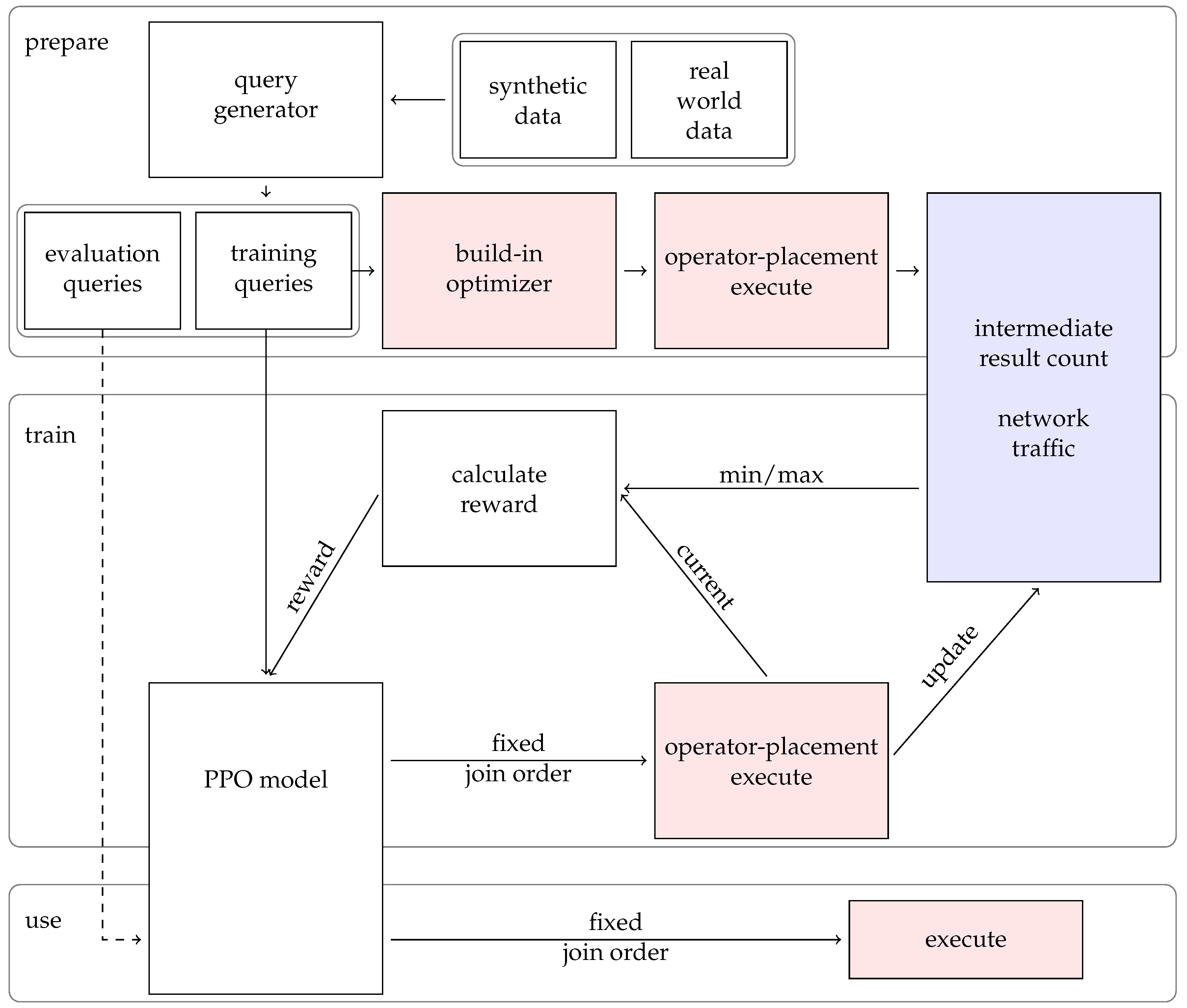
Luposdate3000 [44] (source code available at https://github.com/luposdate3000/luposdate3000 (accessed on 20 August 2022)) is a SPARQL DBMS with a focus on IoT. We ensured that new features can easily extend the DBMS by design. It is entirely written in Kotlin and can therefore be compiled to different targets, allowing it to be executed on various platforms. The database works with the simulator SIMORA [14] to gain further insight into semantic web databases. Luposdate3000 uses column iterators wherever possible when evaluating queries. The overall query processing pipeline can be seen in Figure 2.

Figure 2. Luposdate3000 Join order optimization pipeline. We added or modified the colored parts. In blue, we highlight the added executable scheme, which only outputs statistics instead of actual results. The modified machine learning and network placement are shown in red and green.

We modified the DBMS to return the number of intermediate results for each executed query instead of the actual results. In Figure 2, this is highlighted in blue. Additionally, we added an interface to allow an external application to enforce a specific join tree during execution. This interface is marked in red in Figure 2. In particular, this simplifies interaction with the Python programming language, which plays a central role in the machine learning community.

Luposdate3000 has two built-in join order optimizers: a greedy optimizer and one with dynamic programming. Neither of them uses machine learning. Therefore, they can be used to compare the quality of machine learning approaches with the greedy and dynamic programming-based approaches. The Luposdate3000 greedy join order optimizer uses minimalistic histograms with only one bucket. This simplicity allows the histograms to be extracted directly from the data without additional storage overhead. It also allows the optimizer to always use an up-to-date histogram.

The optimization process itself consists of several steps. First, the optimizer collects all input from all consecutive joins to obtain an overview of what needs to be joined. Then, these inputs are grouped by variable name to detect the star-shaped subtrees first. The basic idea is that this allows merge joins to be used more frequently. In addition to the star join pattern, many identical variable names indicate that the join will likely reduce the number of output rows. Within each group, the optimizer looks at the estimated number of results for each input and the estimated number of different results for each join. The inputs are concatenated so that the estimated output cardinality remains as small as possible. The groups with different variables must be merged in the last step. Here, the optimizer attempts to assemble subgroups with at least one variable in common. This strategy prevents the optimizer from choosing the Cartesian product as long as the SPARQL query allows it. The advantage of this optimizing strategy is that the time needed to find a join tree is linear to the number of inputs to join.

The dynamic programming-based optimizer produces better join trees. However, the time needed to create the join tree is $O(N\ast 2^R)$, with R as the number of inputs to join and N as the number of join orders.

Luposdate3000 supports many widely used indexing strategies such as RDF-3X [32] and Hexastore [33], and many partitioning schemes based on them. Each time a value is inserted into the database or included in the output, a dictionary must be called to translate the internal IDs into their corresponding values. A distributed environment, especially with many devices, generates much traffic. Caching some of the last used values is possible to reduce this traffic. In particular, ontology predicates are used in almost every query. Therefore, we added another cache to the database containing all of the ontology’s values. Last, we encoded small values directly in the internal dictionary IDs so that these values could be decoded without a dictionary. Given the definition of the benchmark scenario, these optimizations make it possible to avoid distributed dictionary access altogether and use only local knowledge. To improve data insertion, the database supports multi-cast-like communication.

3. Our Approach

In our approach, the routing and application layers are tightly coupled. We use the same modifications to the routing layer as in our earlier article [31]. Therefore, we assume that the routing protocol has the necessary information to find the next DBMS on the path to a given DBMS. Therefore, we begin this section by explaining how this information can be used to optimize operator distribution. Finally, the reduced network traffic can further train the model to improve the order of joins.

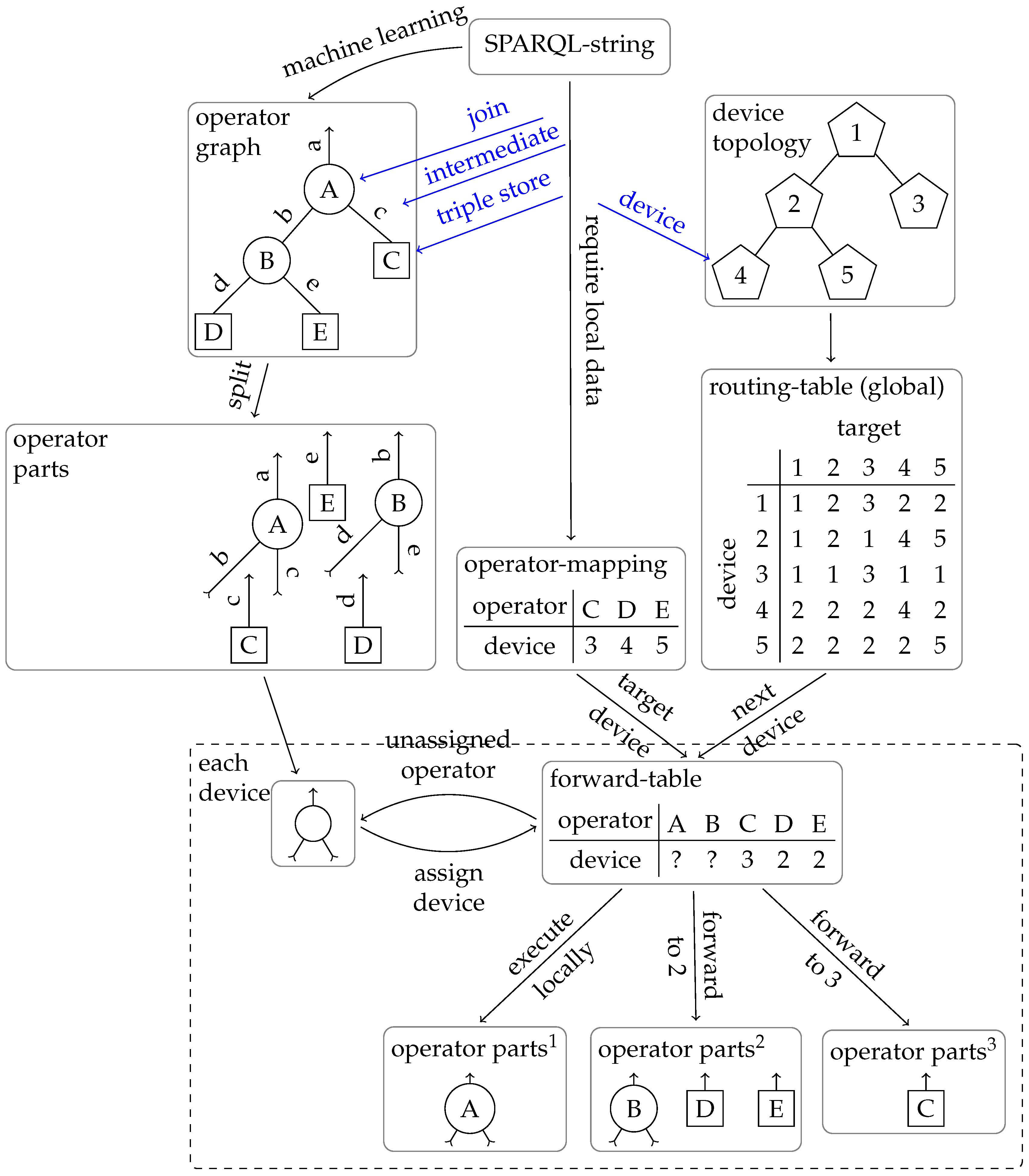
3.1. Query Distribution

Figure 3 shows the processing pipeline of a SPARQL query. This whole chapter explains the details. First, the SPARQL string query must be converted into an operator graph. This conversion is carried out by tokenizing the string and logical optimization. In our case, this is join order optimization using machine learning. The optimization goal is often defined as the estimated execution time, but other metrics, such as network traffic, are also achievable goals.

Figure 3. Routing-assisted join order optimization in comparison to state-of-the-art static join order optimization. Small letters indicate data streams. Capital letters indicate Operators in the operator graph. Numbers are addresses of devices.

After logical optimization, we divide the graph into many parts, with one for each operator. At each point where the operator graph is divided, we add matching send and receive operators, indicated by arrows in the figure. These send-and-receive operators ensure that the operator graph can be executed in a distributed manner.

Then, these parts must be assigned to the devices. The operators for triple store access must be executed on specific devices because they require local data. In the figure, this is represented by the operator mapping table. All other operators could be executed anywhere. Our goal is to shorten the data paths. Therefore, we need to work with the local routing table of our current device. In our example, device 1 is only connected to devices 2 and 3. It cannot send all triple-store operators directly to their destination. Therefore, for each triple store operator, we compute the next device through which it must be routed to reach its destination. This functionality must also be provided within the routing protocol. Therefore, it is helpful if the routing protocol provides these functions. To check where the other operators should be sent, we consider all of the inputs of an operator. This operator is also sent if all inputs are routed to the same device. This process is repeated until each operator is assigned a destination. Operators whose inputs are sent to different devices are calculated locally on the current device. This step is repeated on each device, to which operators are passed until all operators are executed locally on the current device. In this way, the operator graph is adapted to the topology.

During or after the evaluation of a join operator, it is possible to switch the target device again if the result set is larger than the input set. In this case, the input streams and operators are forwarded to the parent DBMS instance. While this increases the CPU load since the join operator must be repeated, it reduces the network load since less data must be sent. This extension can be applied to any operator placement strategy.

3.2. Machine Learning Strategy

There are many different types of machine learning approaches [45]. In the context of join order optimization, manually labeling good or bad join orders does not make sense. Therefore, we are using a reinforcement learning approach, which can improve its model through exploration. Reinforcement learning algorithms are fundamentally online learning approaches. However, there are multiple variations of offline learning as well [45]. In our context, there are three reasons to stop training when the model reaches a good enough state:

• The training requires much CPU or GPU time to update its model. By freezing the model, the required computations can be significantly reduced.
• The statistics data can be removed after training, freeing up much storage space. When the model needs to be retrained because of many updates or different queries, these statistics would be outdated, so there is no reason to keep them after the training.
• We have modified the query executor to return intermediate results instead of the actual response for each query. Counting every intermediate result also requires time and resources, so we want to avoid it. The idea of different details in the data for training and evaluation is also used in other algorithms [46].

3.3. Reinforcement Learning for Join Order Optimization in SPARQL (ReJOOSp)

While the number of tables in SQL is small, the number of predicates in SPARQL is very high. This is a significant difference in possible encoding for machine learning. In SQL, it is enough to say which tables should be joined. On the other hand, in SPARQL, the triple patterns must be explicitly connected, dramatically increasing the input size for machine learning and making it harder for the model to learn what is essential. 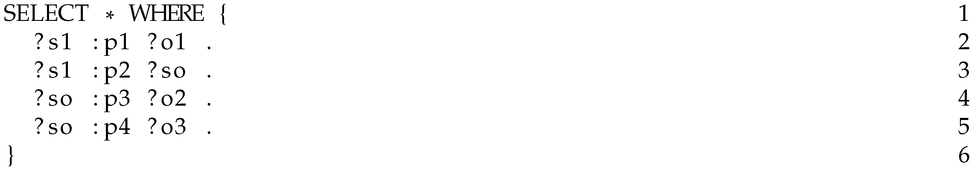Figure 4 shows an example query with two subject–subject joins and one subject–object join. A plausible approach would be to join the subject–subject joins independently from each other first. The assumption here is, that a subject–subject join is often a 1 to 1 join. Additionally, those joins can be evaluated independently. Afterward, both intermediate results are joined.

Figure 4. Example SPARQL query.

We use the Stable Baselines 3 [47] framework because there are many more open-source contributors than other frameworks. Especially, there is a community add-on [48] that extends the built-in PPO model with the possibility of masking. Applying masks to the available actions is crucial for the model to produce good join trees. We use the default MLP policy with two layers and 64 nodes, also used in other join order optimizing articles [49]. Using more layers increases the number of learning steps required since the model must first learn how to use these hidden layers.

We need to keep the training phase short. Otherwise, the changes in the dataset will immediately render the newly trained model useless. We want to treat the machine learning model as a black box. This allows us to focus on encoding the query and computing a reward. The reward should reflect the quality of the join tree compared to other previously executed join trees. Therefore, the algorithm needs to know the best and worst case. Calculating the reward for joins with up to five inputs is straightforward, as traversing all join trees and keeping statistics on the good and the bad is possible.

However, since the model is intended to work with larger joins, for example, with 20 join inputs, this approach will not work, as it is impossible to collect statistics on all possible join trees. To solve this problem, we extend the machine learning pipeline to the concept shown in Figure 5.

Figure 5. Machine learning concept. The blue component uses an external SQL DBMS. The red components are executed within Luposdate3000. The white components are implemented in Python.

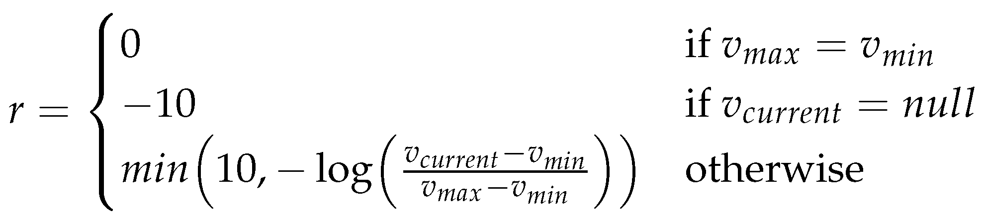
The default optimizer is initially used to initialize the statistics for each SPARQL query. These statistics only map the query to the total network traffic volume. These statistics do not contain specific join orders. Consequently, the model could not learn the competitor’s strategies. Furthermore, whenever we calculate a new reward during training, we extend these statistics with the number of intermediate results produced by the current join plan. All of these statistics about queries and their generated intermediate result counts are stored in a separate SQL DBMS. These statistics will continually improve as the model is trained. The reward calculation function can be seen in Figure 6. The variables $v_{max}$ and $v_{min}$ refer to the min and max network traffic for this specific query, while $v_{current}$ refers to the traffic for the current join plan. Even if the actual best and worst case is unknown, this estimation is good enough to train the model.

Figure 6. Our reward function uses $v_{min}$ and $v_{max}$ from the statistics, which refer to the currently known best- and worst-case network traffic volume. $v_{current}$ may receive a $null$ value when it runs into a timeout. This $null$ value is not considered when calculating the known worst case.

A logarithmic reward function and a minimum compensate for the potentially high variation between different join trees. We generally want to reward good join trees and penalize those whose intermediate results are very high, or the DBMS decides to abort our benchmark because it takes too long.

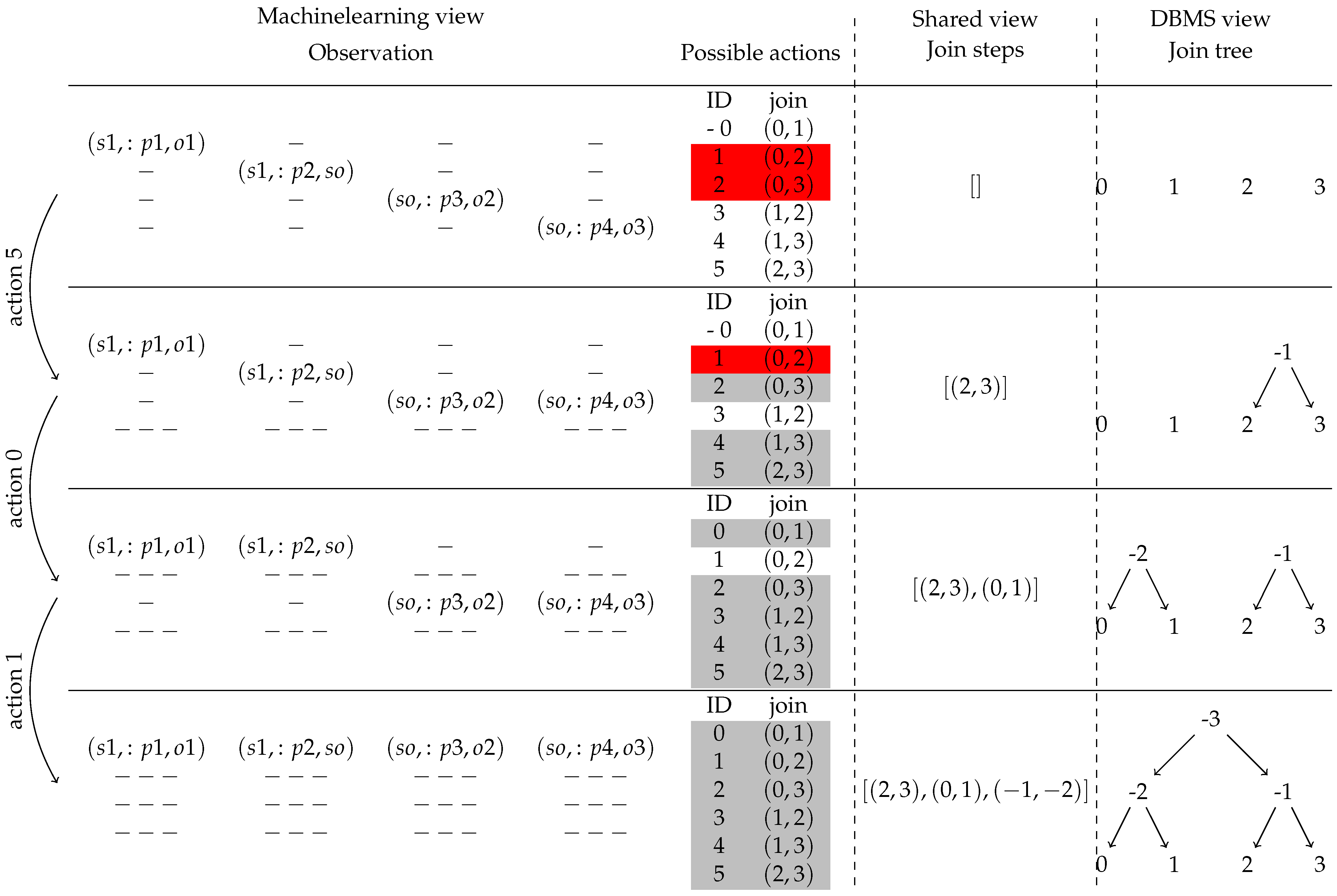
To explain our machine learning approach, ReJOOSp, in detail, we show the internal state of the essential variables in Figure 7. This figure should give an overview of how the join tree is constructed. The details of ReJOOSp are explained in the following. Each row in the figure shows a time step. The essential step in the initialization is the definition of the observation matrix. This observation matrix is created by using a transformation of the SPARQL query, which is placing the triple patterns on the diagonal of a square matrix. This matrix is necessary for the neural network to remember which inputs have already been connected. The remaining cells of this square matrix are marked as empty. The matrix size is chosen such that it is able to represent the largest desired join. This means that the matrix size is quadratic in the maximum number of joins allowed. Even if this seems to be a large matrix, it is still small compared to approaches from relational database systems, where the matrix size is quadratic to the number of tables. The purpose of the matrix is that each join is mapped to a sequence of numbers of the same size. The DBMS itself does not need this observation matrix.

Figure 7. Overview of join order optimization. The gray actions are invalid because the contained relations are already joined. The red actions are Cartesian products, which are avoided.

We define the possible actions as a list of pairs of rows in the matrix that could be joined. To further reduce the machine learning search space, we ignore the difference between the left and right input of the join operator. For the example in Figure 4 with four triple patterns, this list of possible actions can be seen in the top row of Figure 7, next to the observation matrix. In Figure 7, the invalid actions are marked in gray. The Cartesian products are shown in red. The machine learning model now receives the matrix and the action list and selects a new action until only one action is possible. Then, this last action is applied, and the join tree is complete. For each selected action, the step function is executed.

The step function first calculates which two inputs are to be joined. The action ID is looked up in the action list to do this. Then, the observation matrix is updated. Therefore, the values from the matrix line of the right join input are copied to the matrix line of the left join input. All empty fields are skipped so that existing data are not overwritten. Finally, the right hand side join input row is marked as invalid, to prevent it from being considered for joining again. Then, we append our currently selected join step to the join step list. This list of join steps is the target of ReJOOSp, as it is the only output passed to the DBMS at the end. The DBMS can use this list to build the join tree shown in the right column of Figure 7. We are finished when the entire matrix, except for the first row, is cleared. The matrix always ends up in this state, regardless of the chosen join order.

3.4. Weak Points

The machine learning model is expected to work best on queries with the same or similar number of joins as in the training set. When the join count per query is highly varied, multiple models targeting different numbers of joins in a query should be trained. However, it should be noted that traditional approaches cannot deliver good join orders for queries with many joins.

The model needs to be retrained when the data change too much. It costs a lot of computation time whenever a model needs to be retrained. However, optimizing individual queries is cheaper, and the join orders are better than other approaches, such that the computational overhead is reduced at other places in the DBMS.

4. Evaluation

SIMORA [14] (source code available at https://github.com/luposdate3000/SIMORA (accessed on 20 August 2022)) is used to simulate the DBMS in a reproducible randomized topology. This topology was chosen because it is the most realistic one. We apply the operator placement strategy as described in the previous section. We also use that placement strategy when evaluating the join orders given by other DBMSs. The distributed parking scenario benchmark [50] generates 9923 triples to obtain and compare plausible network loads. Since the insertion is independent of the join order, the data transmission to store the data is not included. Due to the simulation component, the execution is much slower, so only joins with up to six triple patterns can be analyzed.

The smaller number of triple patterns allows, as a side effect, for a much shorter training phase. During all measurements, the DBMS distributed the data based on subject hashes because this allows many star-shaped join operators to be executed locally. Figure 8 shows the reward received by the model after x iterations. After about 8192 steps, each model frequently receives a high reward. Frequent high rewards indicate that the model is finished with the training phase.

Figure 8. This figure shows the reward for the model after x training steps. The displayed graphs use an average running function reset after logarithmic increasing distances. The graph names of the models contain the number of triple patterns used during training.

In the current implementation, the training and testing phase queries are disjointed. The evaluation of the evaluation query set confirms that the quality of the join orders does not improve significantly with extended training. Using a maximum of six triple patterns has the advantage of executing all possible join orders and storing their intermediate results and network traffic. To avoid bad results, a timeout of one minute is applied. In addition, all join orders with Cartesian products are terminated immediately. If a query fails this way, the reward calculation assumes twice the worst-case number of intermediate results and network traffic. These complete statistical data are used to evaluate the quality of the join trees computed by the different algorithms.

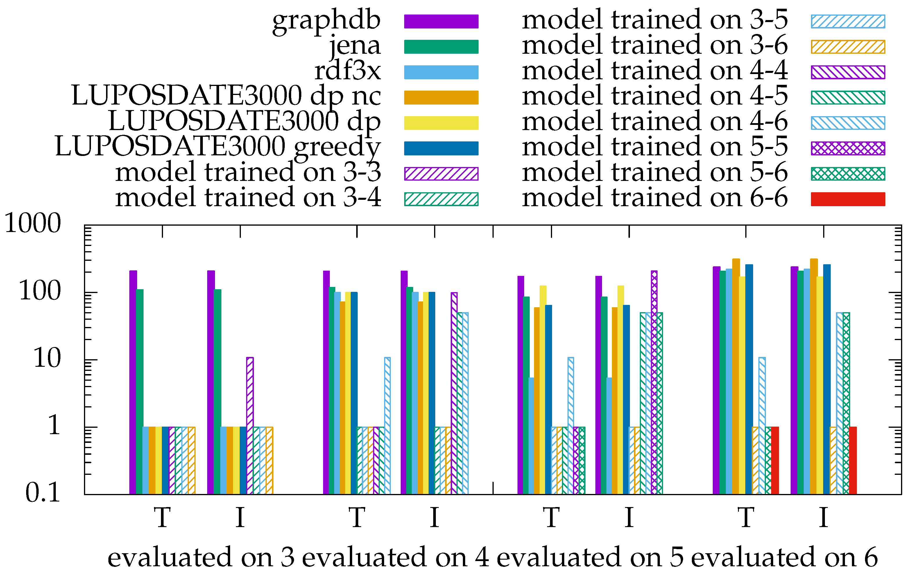
First, the results for the evaluation based on intermediate results are shown in Figure 9. The optimizers from Jena and GraphDB consider only left-deep join orders. However, if only three triple patterns exist, this still matches all possibilities. Nevertheless, these two optimizers always produce about 100 times more intermediates than necessary. The optimizer of RDF3X achieves much better results. It can always select the best case for three triple pattern queries and frequently for five triple patterns. However, the four and six triple-pattern queries achieve bad results like the previous optimizers.

Figure 9. All optimizers were evaluated based on the produced intermediate results. The X-axis shows which evaluation was performed on how many triple patterns. I means intermediate results, and T means network traffic. The Y-axis shows the average factor between the best join order and the chosen join order of a given join order optimizer. A factor of 1 is achieved if the optimizer always chooses the best case. The models are trained on joins with the number of triple patterns specified in their labels.

Luposdate3000 provides two optimizers: dynamic programming (dp in the figure) and greedy programming. The dynamic programming optimizer can optionally cluster the triple patterns by variable names, which reduces the search space, and increases the optimization speed. In the figure, the optimizer marked with nc is not using clustering by variable names. In the context of three triple patterns, all LUPOSDATE3000 built-in optimizers always choose the best join order. However, with more triple patterns, the optimizer achieves a similar quality to the other optimizers without ML. When trained on network traffic, the ML models almost always choose the optimal join order. However, when the reward function during training is based on intermediate results, the optimizer creates unnecessary work.

Next, Figure 10 shows the results for the same queries, but this time the ranking is based on network traffic. The overhead factor is generally much lower than the previous figure showing the intermediate results. This reduction is achieved by the dynamic operator relocation, which first executes the join. Then, the bytes of the input are compared with those of the output. Finally, the option with fewer bytes is chosen and sent over the network.

Figure 10. All optimizers were evaluated based on the network traffic. The X-axis shows which evaluation was performed on how many triple patterns. I means intermediate results, and T means network traffic. The Y-axis shows the average factor between the best join order and the chosen join order of a given join order optimizer. A factor of 1 is achieved if the optimizer always chooses the best case. The models are trained on joins with the number of triple patterns specified in their labels.

Consequently, the only overhead is the operator graph size, sent twice for every device on the path. Since only the network traffic counts in this comparison, and the smaller number is always chosen, there is no advantage for any specific optimizer. Without this optimization, the bad join orders would be much worse than they are now. It is also possible that the ranking between excellent and bad join orders changes by turning off this feature. However, in that case, the absolute number of bytes sent through the network will increase, so those join orders can not be called optimal anymore.

The exciting part of this figure is that the trained model almost always achieves less network traffic than the state-of-the-art static optimizers. When the models are trained on network traffic, their result is almost optimal. They are also slightly better than those models trained on intermediate results. The best possible results were achieved with the model, which trained on all possible mixed triple pattern sizes. Consequently, the figure also shows that overfitting occurs if the models are trained on small query sets, slightly decreasing the quality.

5. Summary and Future Work

We discovered that we can improve the join order quality by using the network traffic volume to train the machine learning model. Our strategy, which pushes the operators as close as possible to the data source, minimizes the produced network traffic by 10%. Alternatively, the model can reduce the number of intermediate results by a factor of 100.

In the future, the machine learning approach could be extended to predict when it has to be retrained due to changes in the data. Several components of this work can be exchanged, such as the dataset, the triple store indices, the topology, the routing protocols, and the encodings for machine learning. Also, using quantum computing instead of traditional machine learning could be considered.