
How Machine Learning Classification Accuracy Changes in a Happiness Dataset with Different Demographic Groups


Abstract
:1. Introduction
2. Related Works
3. Methods
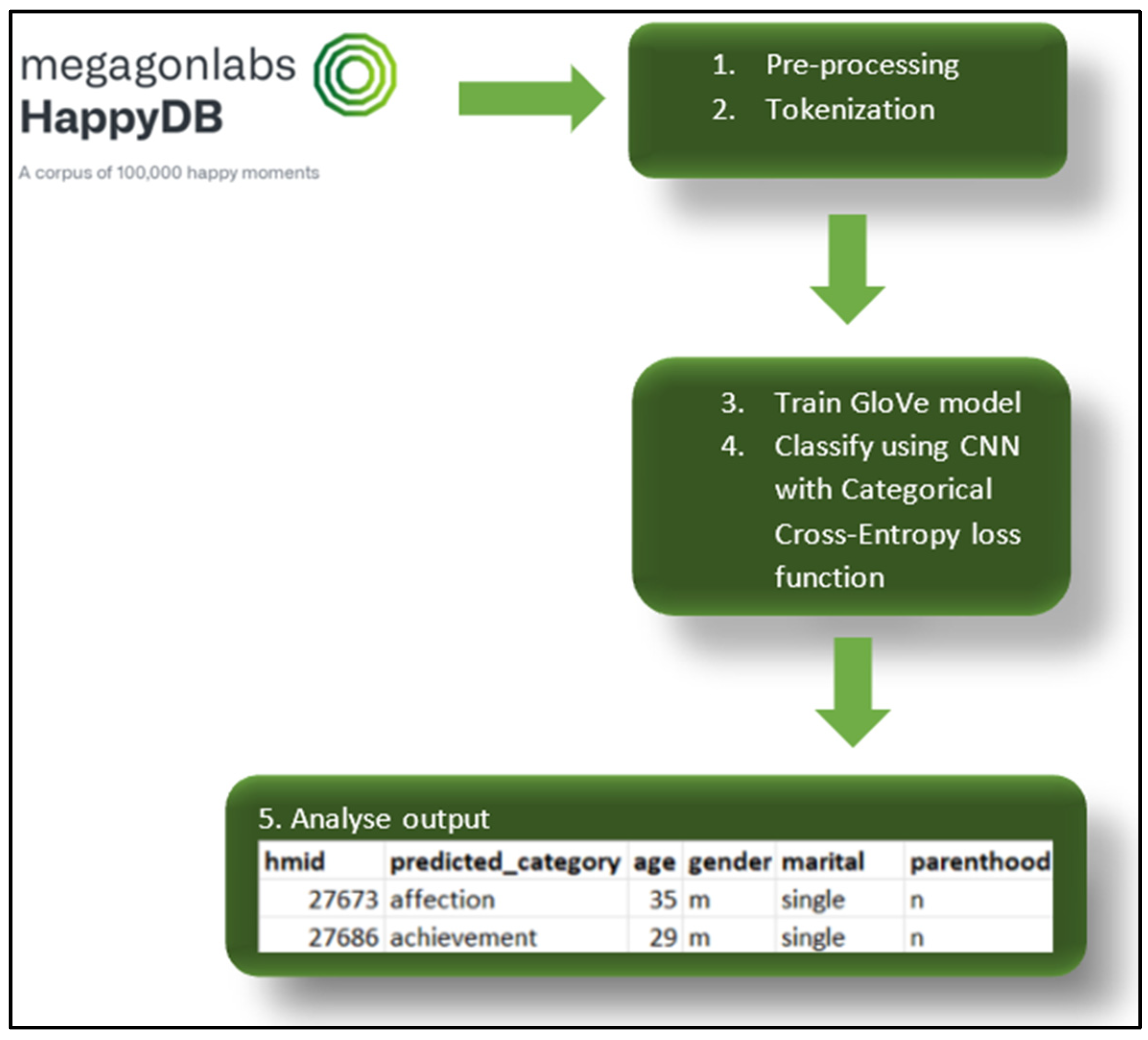
3.1. Dataset
3.2. Data Science Pipeline
3.3. Classification Evaluation
3.3.1. Classification Accuracy
3.3.2. Precision
3.3.3. Classifier Recall
3.3.4. F-Measure Metric
3.4. Training Classifiers on Seven Categories of Happiness
3.5. Test Dataset Imbalance
4. Results
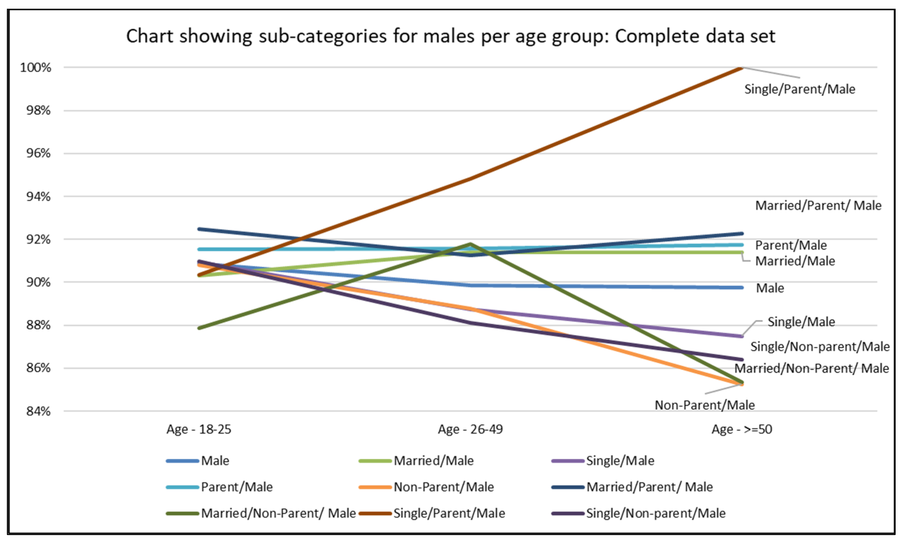
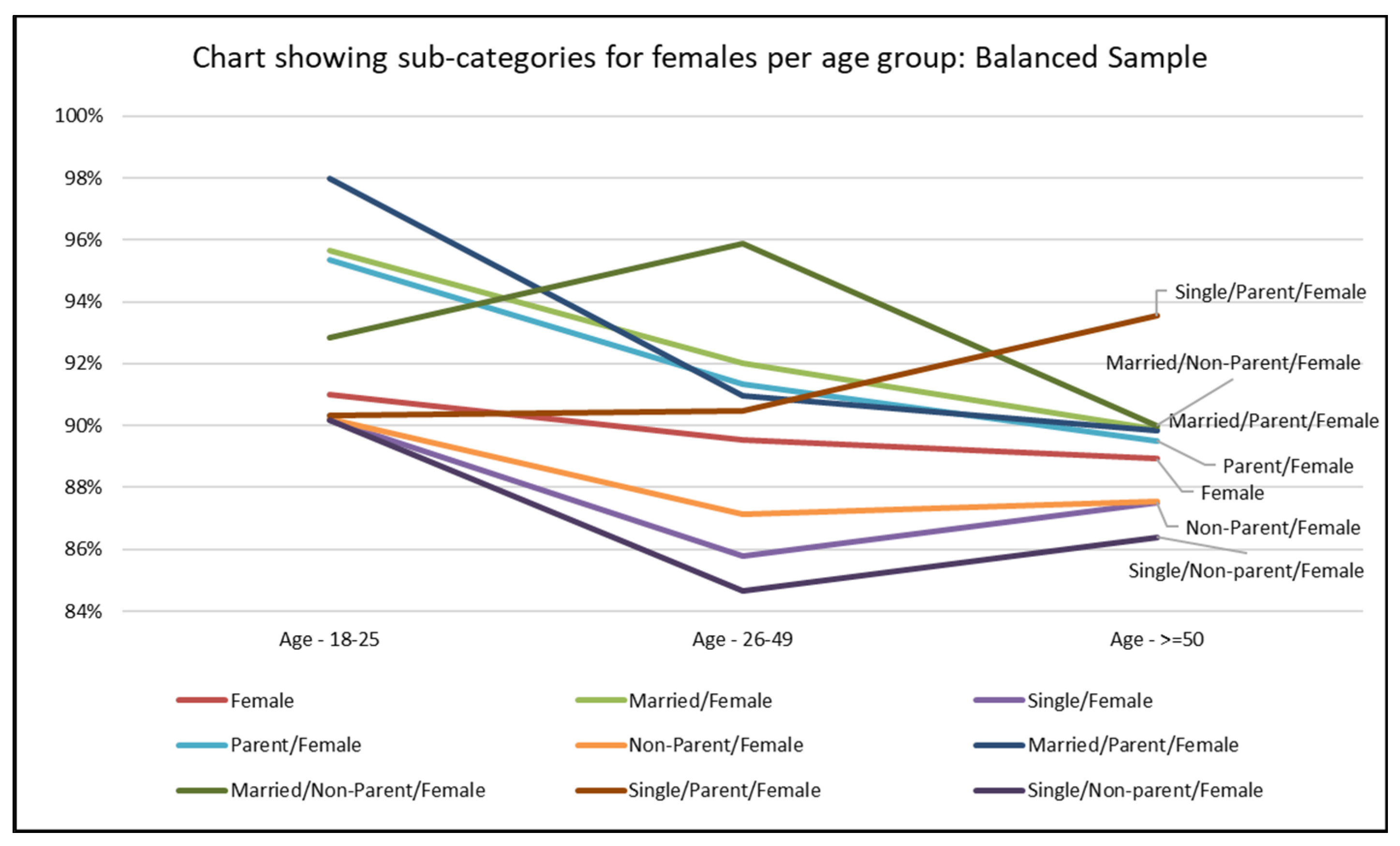
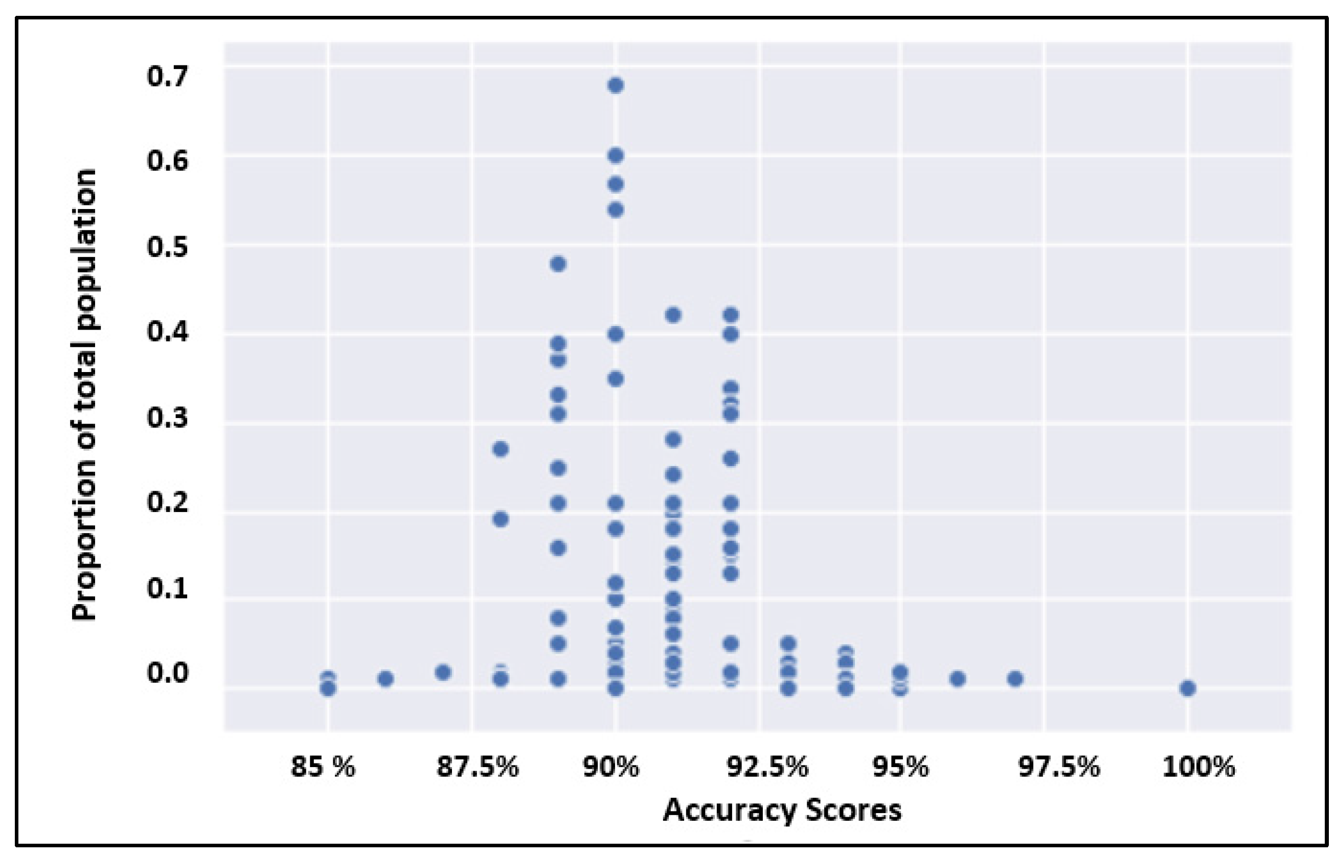
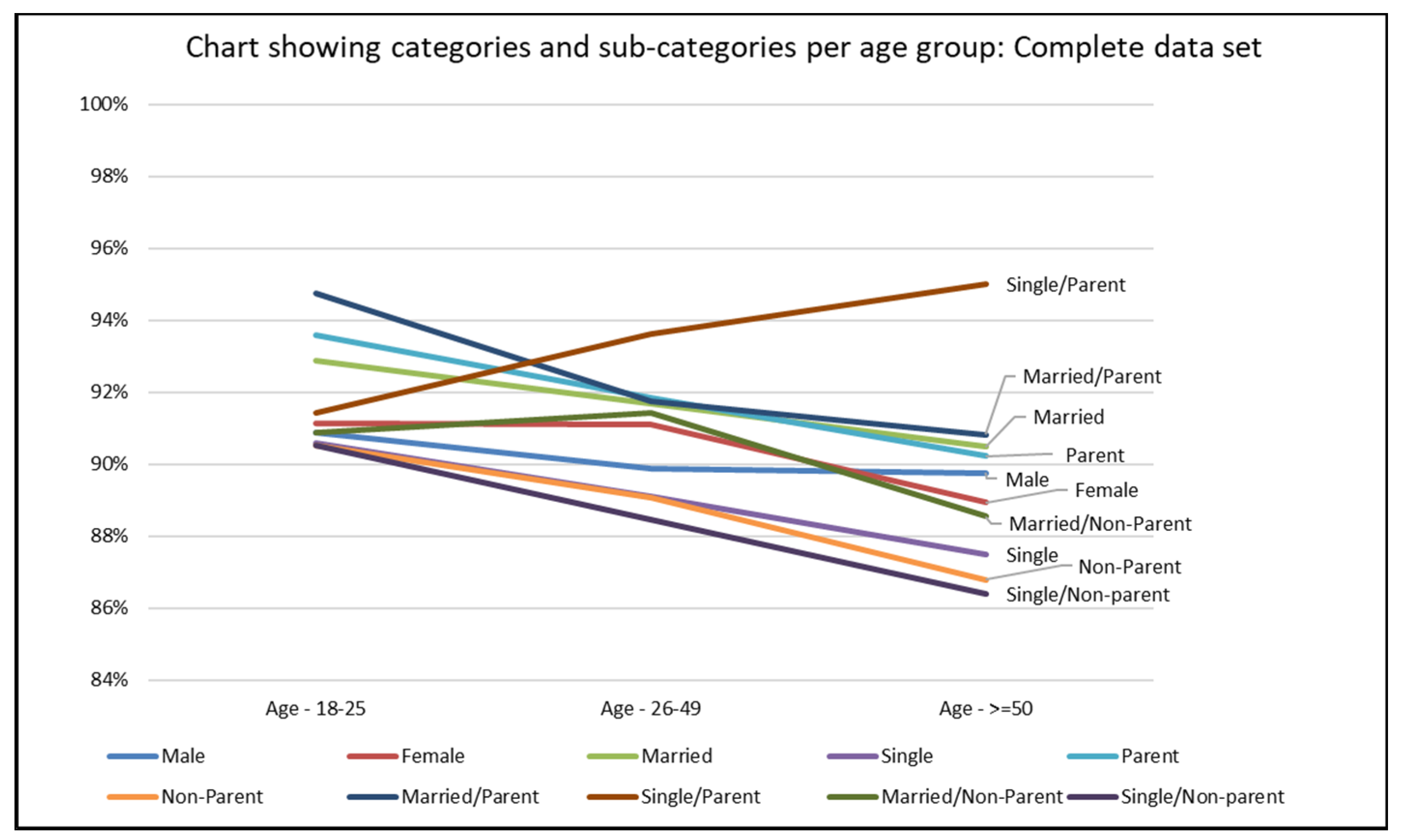
Displaying Prediction Accuracy for a Classification Task by Predicting for Different Demographic Groups
5. Discussion
6. Limitations
7. Conclusions
Author Contributions
Funding
Institutional Review Board Statement
Informed Consent Statement
Data Availability Statement
Conflicts of Interest
References
- Compton, W.; Hoffman, E. Positive Psychology: The Science of Happiness and Flourishing, 3rd ed.; Sage Publications: Thousand Oaks, CA, USA, 2013. [Google Scholar]
- Mohamed, E.; Mostafa, S. Computing Happiness from Textual Data. Stats 2019, 2, 347–370. [Google Scholar] [CrossRef] [Green Version]
- Vashisth, P.; Meehan, K. Gender Classification using Twitter Text Data. In Proceedings of the 31st Irish Signals and Systems Conference, Cork, Ireland, 9–10 June 2020. [Google Scholar]
- O’Neil, C. Weapons of Math Destruction: How Big Data Increases Inequality and Threatens Democracy. Vikalpa 2019, 44, 97–98. [Google Scholar]
- Sweeney, C.; Ennis, E.; Bond, R.; Mulvenna, M.; O’Neill, S. Understanding a Happiness Dataset: How the Machine Learning Classification Accuracy Changes with Different Demographic Groups. In Proceedings of the 2021 IEEE Symposium on Computers and Communications (ISCC ‘21), Athens, Greece, 5 September 2021. [Google Scholar]
- Akari, A.; Evensen, S.; Golshan, B.; Halevy, A.; Li, V.; Lopatenko, A.; Stepanov, D.; Suhara, Y.; Tan, W.-C.; Xu, Y. Happydb: A Corpus of 100,000 Crowdsourced Happy Moments. arXiv 2018, arXiv:1801.07746. [Google Scholar]
- Raj Kumar, G.; Bhattacharya, P.; Yang, Y. What Constitutes Happiness? Predicting and Characterizing the Ingredients of Happiness Using Emotion Intensity Analysis. Available online: http://ceur-ws.org/Vol-2328/4_3_paper_22.pdf (accessed on 26 May 2020).
- Jaidka, K.; Mumick, S.; Chhaya, N.; Ungar, L. The CL-Aff Happiness Shared Task: Results and Key Insights. Available online: http://ceur-ws.org/Vol-2328/2_paper.pdf (accessed on 27 May 2020).
- Siriaraya, P.; Suzuki, K.; Nakajima, S. Utilizing Collaborative Filtering to Recommend Opportunities for Positive Affect in Daily Life. In Proceedings of the HealthRecSys@ RecSys, Copenhagen, Denmark, 20 September 2019; pp. 2–3. [Google Scholar]
- Torres, J.; Vaca, C. Neural Semi-Supervised Learning for Multi-Labeled Short-Texts. In Proceedings of the 2nd Workshop on Affective Content Analysis@ AAAI (AffCon2019), Honolulu, HI, USA, 27 January 2019. [Google Scholar]
- Veenhoven, R.; Bakker, A.; Burger, M.; Van Haren, P.; Oerlemans, W. Effect on Happiness of Happiness Self-monitoring and Comparison with Others. In Positive Psychology Interventions: Theories, Methodologies and Applications within Multi-Cultural Contexts; VanZyl, L., Rothmann, S., Eds.; Springer International: Hillerød, Denmark, 2019; pp. 1–23. [Google Scholar]
- Klonsky, E.; May, A. The Three-Step Theory (3ST): A New Theory of Suicide Rooted in the “Ideation-to-Action” Framework. Int. J. Cogn. Ther. 2015, 8, 114–129. [Google Scholar] [CrossRef] [Green Version]
- Gillick, D. Can Conversational Word Usage Be Used to Predict Speaker Demographics? In Proceedings of the Eleventh Annual Conference of the International Speech Communication Association, Makuhari, Japan, 26–30 September 2010. [Google Scholar]
- Koppel, M.; Argamon, S.; Shimoni, A. Automatically Categorizing Written Texts by Author Gender. Lit. Linguist. Comput. 2002, 17, 401–412. [Google Scholar] [CrossRef]
- Schler, J.; Koppel, M.; Argamon, S.; Pennebaker, J. Effects of Age and Gender on Blogging. In Proceedings of the 2006 AAAI Spring Symposium on Computational Approaches for Analyzing Weblogs, Palo Alto, CA, USA, 27–29 March 2006. [Google Scholar]
- Filippova, K. User Demographics and Language in an Implicit Social Network. In Proceedings of the 2012 Joint Conference on Empirical Methods in Natural Language Processing and Computational Natural Language Learning (EMNLP-CoNLL ‘12), Jeju Island, Korea, 12–14 July 2012. [Google Scholar]
- Herring, S.; Paolillo, H.J. Gender and Genre Variation in Weblogs. J. Socioling. 2006, 10, 439–459. [Google Scholar] [CrossRef]
- Huffaker, D.A.; Calvert, S. Gender, Identity and Language Use in Teenager Blogs. J. Comput.-Mediat. Commun. 2005, 10, 10211. [Google Scholar]
- Burger, J.D.; Henderson, J. An Exploration of Observable Features Related to Blogger Age. In Proceedings of the 2006 AAAI Spring Symposium on Computational Approaches for Analyzing Weblogs, Palo Alto, CA, USA, 27–29 March 2006. [Google Scholar]
- Yan, X.; Yan, L. Gender Classification of Weblogs Authors. In Proceedings of the 2006 AAAI Spring Symposium on Computational Approaches for Analyzing Weblogs, Palo Alto, CA, USA, 27–29 March 2006. [Google Scholar]
- Popescu, A.; Grefenstette, G. Mining User Home Location and Gender from Flickr Tags. In Proceedings of the International Conference on Weblogs and Social Media (ICWSM-10), Washington, DC, USA, 23–26 May 2010. [Google Scholar]
- Kincaid, J.P.; Fishburne, R.P., Jr.; Rogers, R.L.; Chissom, B.S. Derivation of New Readability Formulas (Automated Readability Index, Fog Count and Flesch Reading Ease Formula) for Navy Enlisted Personnel; Research Branch Report; Naval Technical Training: Meridian, MS, USA, 1975. [Google Scholar]
- Mishra, P. 4 Popular Techniques to Measure the Readability of a Text Document. Available online: https://medium.com/mlearning-ai/4-popular-techniques-to-measure-the-readability-of-a-text-document-32a0882db6b2 (accessed on 2 November 2021).
- Mikolov, T.; Chen, K.; Corrado, G.; Dean, J. Efficient Estimation of Word Representations in Vector Space. arXiv 2013, arXiv:1301.3781. [Google Scholar]
- Pennington, J.; Socher, R.; Manning, C. GloVe: Global Vectors for Word Representation. In Proceedings of the Conference on Empirical Methods on Natural Language Processing (EMNLP ‘14), Doha, Qatar, 26–28 October 2014. [Google Scholar]
- Lewis, D. Representation and Learning in Information Retrieval. Ph.D. Thesis, University of Massachusetts, Amherst, MA, USA, 1992. [Google Scholar]
- Pak, A.; Paroubek, P. Twitter as a Corpus for Sentiment Analysis and Opinion Mining. In Proceedings of the International Conference on Language Resources and Evaluation (LREC ’10), Valletta, Malta, 17–23 May 2010. [Google Scholar]
- Melville, P.; Gryc, W.; Lawrence, R. Sentiment Analysis of Blogs by Combining Lexical Knowledge with Text Classification. In Proceedings of the 15th ACM SIGKDD International Conference on Knowledge Discovery and Data Mining, Paris, France, 28 June–1 July 2009. [Google Scholar]
- Ke, G.; Meng, Q.; Finley, T.; Wang, T.; Chen, W.; Ma, W.; Ye, Q.; Liu, T. Lightgbm: A Highly Efficient Gradient Boosting Decision Tree. In Proceedings of the 31st Conference on Neural Information Processing Systems (NIPS 2017), Long Beach, CA, USA, 4–9 December 2017. [Google Scholar]
- Safavian, S.; Landgrebe, D. A Survey of Decision Tree Classifier Methodology. IEEE Trans. Syst. Man Cybern. 1991, 21, 660–674. [Google Scholar] [CrossRef] [Green Version]
- Gu, J.; Wang, Z.; Kuen, J.; Ma, L.; Shahroudy, A.; Shuai, B.; Liu, T.; Wang, X.; Wang, G.; Cai, J.; et al. Recent Advances in Convolutional Neural Networks. Pattern Recognit. 2018, 77, 354–377. [Google Scholar] [CrossRef] [Green Version]
- Tiwari, V.; Lennon, R.; Dowling, T. Not Everything You Read Is True! Fake News Detection using Machine learning Algorithms. In Proceedings of the 2020 31st Irish Signals and Systems Conference (ISSC), Letterkenny, Ireland, 11–12 June 2020. [Google Scholar]
- Li, Y.; Sun, G.; Zhu, Y. Data Imbalance Problem in Text Classification. In Proceedings of the 2010 Third International Symposium on Information Processing, Qingdao, China, 15–17 October 2010. [Google Scholar]


| Category | Definition | Examples |
|---|---|---|
| Achievement | Employing extra effort to achieve a better-than-expected result. | Finish work. Complete marathon. |
| Affection | Meaningful interaction with family, loved ones, and pets. | Hug. Cuddle. Kiss. |
| Bonding | Meaningful interactions with friends and colleagues. | Have meals with coworkers. Meet friends. |
| Enjoying the Moment | Being aware or reflecting on the present environment. | Have a good time. Mesmerize. |
| Exercise | Intent to exercise or workout. | Run. Bike. Do yoga. Lift weights. |
| Leisure | An activity performed regularly in one’s free time for pleasure. | Play games. Watch movies. Bake cookies. |
| Nature | In the open air, in nature. | Garden. Beach. Sunset. Weather. |
| Category | Count: Total Dataset | Count: Train | Count: Test |
|---|---|---|---|
| Affection | 34,168 | 27,372 | 6796 |
| Achievement | 33,993 | 27,211 | 6782 |
| Enjoying the Moment | 11,144 | 8905 | 2239 |
| Bonding | 10,727 | 8609 | 2118 |
| Leisure | 7458 | 5922 | 1536 |
| Nature | 1843 | 1456 | 387 |
| Exercise | 1202 | 953 | 249 |
| Total | 100,535 | 80,428 | 20,107 |
| Naive Bayes | Gradient Boosting | CNN | |
|---|---|---|---|
| Accuracy | 82.48% | 86.02% | 90.83% |
| Recall | 0.85 | 0.87 | 0.89 |
| Precision | 0.86 | 0.89 | 0.90 |
| F1 | 0.854 | 0.883 | 0.897 |
| Group Name | All Ages | 18–25 | 26–49 | >=50 |
|---|---|---|---|---|
| Male | 90.13% | 90.88% | 89.86% | 89.76% |
| n | 11,555 | 3017 | 8011 | 508 |
| Female | 90.83% | 91.141% | 91.09% | 88.93% |
| n | 8422 | 1761 | 5645 | 1003 |
| Married | 91.62% | 92.87% | 91.68% | 90.48% |
| n | 8351 | 561 | 6886 | 893 |
| Single | 89.63% | 90.58% | 89.09% | 87.50% |
| n | 10,763 | 4236 | 6196 | 312 |
| Parent | 91.72% | 93.58% | 91.83% | 90.23% |
| n | 7981 | 514 | 6389 | 1064 |
| Non-Parent | 89.50% | 90.54% | 89.07% | 86.78% |
| n | 12,119 | 4301 | 7346 | 454 |
| Married/Male | 91.33% | 90.32% | 91.40% | 91.41% |
| n | 4174 | 279 | 3569 | 326 |
| Single/Male | 89.57% | 90.94% | 88.74% | 87.50% |
| n | 7050 | 2737 | 4182 | 112 |
| Married/Female | 91.96% | 95.39% | 92.06% | 89.88% |
| n | 4130 | 282 | 3274 | 563 |
| Single/Female | 89.88% | 90.27% | 89.83% | 87.50% |
| n | 3637 | 1460 | 1977 | 200 |
| Married/Parent | 91.76% | 94.76% | 91.76% | 90.81% |
| n | 6288 | 286 | 5230 | 762 |
| Single/Parent | 93.23% | 91.43% | 93.61% | 95.00% |
| n | 1019 | 210 | 767 | 40 |
| Parent/Male | 91.60% | 91.54% | 91.59% | 91.76% |
| n | 3680 | 260 | 3066 | 352 |
| Non-Parent/Male | 89.43% | 90.82% | 88.79% | 85.26% |
| n | 7871 | 2755 | 4943 | 156 |
| Parent/Female | 91.88% | 95.67% | 92.13% | 89.52% |
| n | 4239 | 254 | 3267 | 706 |
| Non-Parent/Female | 89.76% | 90.38% | 89.64% | 87.54% |
| n | 4180 | 1507 | 2375 | 297 |
| Married/Non-Parent | 91.16% | 90.88% | 91.41% | 88.55% |
| n | 2059 | 274 | 1653 | 131 |
| Single/Non-parent | 89.25% | 90.53% | 88.45% | 86.40% |
| n | 9741 | 4025 | 5427 | 272 |
| Married/Parent/ Male | 91.41% | 92.47% | 91.25% | 92.28% |
| n | 2991 | 146 | 2560 | 285 |
| Married/Non-Parent/ Male | 91.11% | 87.88% | 91.77% | 85.37% |
| n | 1181 | 132 | 1008 | 41 |
| Married/Parent/Female | 92.16% | 97.14% | 92.35% | 89.85% |
| n | 3251 | 140 | 2628 | 473 |
| Married/Non-Parent/Female | 91.22% | 93.66% | 90.84% | 90.00% |
| n | 877 | 142 | 644 | 90 |
| Single/Parent/Male | 93.92% | 90.35% | 94.81% | 100.00% |
| n | 510 | 114 | 385 | 9 |
| Single/Parent/Female | 92.56% | 92.71% | 92.43% | 93.55% |
| n | 497 | 96 | 370 | 31 |
| Single/Non-parent/Male | 89.23% | 90.96% | 88.12% | 86.41% |
| n | 6538 | 2622 | 3796 | 103 |
| Single/Non-parent/Female | 89.46% | 90.10% | 89.23% | 86.39% |
| n | 3139 | 1364 | 1606 | 169 |
Publisher’s Note: MDPI stays neutral with regard to jurisdictional claims in published maps and institutional affiliations. |
© 2022 by the authors. Licensee MDPI, Basel, Switzerland. This article is an open access article distributed under the terms and conditions of the Creative Commons Attribution (CC BY) license (https://creativecommons.org/licenses/by/4.0/).
Share and Cite
Sweeney, C.; Ennis, E.; Mulvenna, M.; Bond, R.; O’Neill, S. How Machine Learning Classification Accuracy Changes in a Happiness Dataset with Different Demographic Groups. Computers 2022, 11, 83. https://doi.org/10.3390/computers11050083
Sweeney C, Ennis E, Mulvenna M, Bond R, O’Neill S. How Machine Learning Classification Accuracy Changes in a Happiness Dataset with Different Demographic Groups. Computers. 2022; 11(5):83. https://doi.org/10.3390/computers11050083
Chicago/Turabian StyleSweeney, Colm, Edel Ennis, Maurice Mulvenna, Raymond Bond, and Siobhan O’Neill. 2022. "How Machine Learning Classification Accuracy Changes in a Happiness Dataset with Different Demographic Groups" Computers 11, no. 5: 83. https://doi.org/10.3390/computers11050083
APA StyleSweeney, C., Ennis, E., Mulvenna, M., Bond, R., & O’Neill, S. (2022). How Machine Learning Classification Accuracy Changes in a Happiness Dataset with Different Demographic Groups. Computers, 11(5), 83. https://doi.org/10.3390/computers11050083