Abstract
Several calibration algorithms use spheres as calibration tokens because of the simplicity and uniform shape that a sphere presents across multiple views, along with the simplicity of its construction. Among the alternatives are the use of complex 3D tokens with reference marks, usually complex to build and analyze with the required accuracy; or the search of common features in scene images, with this task being of high complexity too due to perspective changes. Some of the algorithms using spheres rely on the estimation of the sphere center projection obtained from the camera images to proceed. The computation of these projection points from the sphere silhouette on the images is not straightforward because it does not match exactly the silhouette centroid. Thus, several methods have been developed to cope with this calculation. In this work, a simple and fast numerical method adapted to precisely compute the sphere center projection for these algorithms is presented. The benefits over other similar existing methods are its ease of implementation and that it presents less sensibility to segmentation issues. Other possible applications of the proposed method are presented too.
1. Introduction
Spheres are commonly employed as calibration tokens in several camera calibration algorithms [1,2,3,4,5,6,7,8]. The main reason for this is that they show a similar silhouette (elliptical shape) independent of the camera position. An interesting review of the methods using spheres for this purpose can be found in [1].
Typically, the center of the sphere silhouette obtained by a camera is used to estimate the sphere center projection. Nevertheless, this is not an exact estimation because the sphere center projection does not exactly match the silhouette center on the image plane (see Figure 1); therefore, an error, referred to as eccentricity [9,10], is committed if the mass center of the sphere projection is used. The magnitude of this error depends on several parameters: the sphere radius, camera–sphere distance, camera focal length, camera angle, etc. The computation of the exact center projection is not as straightforward as computing the center of the sphere silhouette on the image and requires more computation time; thus, obtaining an estimation of this error can be interesting in order to decide whether it could be neglected or a correction is necessary.
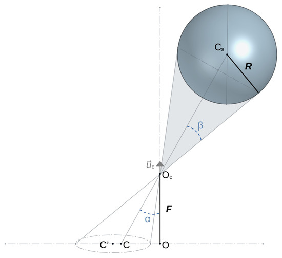
Figure 1.
A sphere of center is projected on the camera plane as an ellipse. The projection of its center, C, does not lie exactly on the ellipse center, . F represents the camera focal length, is the camera position and is the camera orientation. O, principal point of camera image.
To solve this problem, the camera’s intrinsic and extrinsic parameters, along with the sphere radius and some information derived from the sphere silhouette, are needed. In [11], the equation of the silhouette (an ellipse) is employed and an analytical solution is developed. In [1,12], an approximate and an analytical solution are, respectively, derived from the ellipse center and area. These methods compute the sphere position in the space, but, if needed, the eccentricity can be derived. In [9], the eccentricity is directly computed by developing a formula from the silhouette equation. Finally, in other works [4], the corrections are integrated into the calibration procedure equations as it is not possible to access directly the correction.
All these works present complex formulations and rely on segmentation image or edge detection algorithms to obtain silhouette information. Accuracy issues occur with the estimation of the ellipse equation or the ellipse area on poorly illuminated environments or when reflecting objects appear.
In the present work, a variation of these methods is introduced using part of the fixed parameters (intrinsic camera parameters and sphere radius), the silhouette center and an estimation of the camera-to-sphere distance. This approach simplifies calculations and is more adequate for camera calibration algorithms such as the one presented in [3]. Furthermore, the silhouette center computed as the mass center of the silhouette is less sensitive to segmentation issues.
The remainder of this paper is organized as follows: In Section 2, the new approach is presented. In Section 3, an evaluation of the error in the context of the calibration method presented in [3] is performed, and the calibration results are compared by employing exact sphere center projection. In Section 4, the conclusions are presented.
2. Sphere Center Projection
The projection of a sphere in a plane is an ellipse, but, as shown in Figure 1, the sphere center projection C does not match the ellipse center .
Considering a pinhole camera model, knowing the sphere center position () and the intrinsic and extrinsic camera parameters (F, and ; see Figure 1), the C value can be easily computed as the intersection of the line defined by and the plane defined by and O (camera principal point) by means of classic geometry [13,14].
On the other hand, computing is not so straightforward, but it can be calculated by means of trigonometry. Knowing the angles and (see Figure 1 and Figure 2), can be computed as
where
and is a unitary vector that can be computed as
because and C are collinear, with the ellipse’s major axis passing through the camera principal point O ( 1 in [1]).
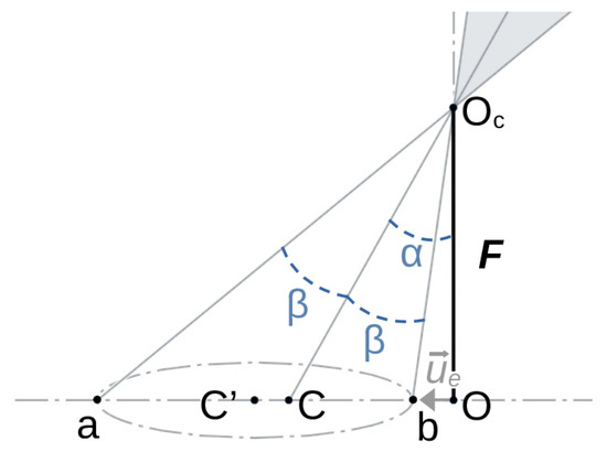
Figure 2.
Point can be computed as the mean of points a and b.
Following the calculation in [9], the angle can be computed from the working distance (W, sphere-to-camera distance) and the sphere radius (R) using triangle similarity as follows (Figure 3):
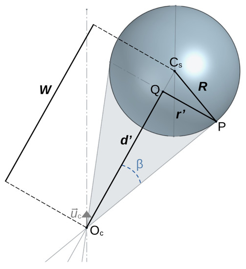
Figure 3.
Triangles and and triangles and are similar.
On the other hand, angle can be computed (see Figure 1) as the angle between the camera orientation, , and the vector pointing to the sphere center from the camera, , as
All these values can be computed if the sphere position is known; however, this is not the case in a calibration context, where only an estimation of the camera parameters, sphere dimension and 2D sphere images is available. In the present work, a method to compute the real sphere center projection on an image, C, is proposed employing the available information (intrinsic camera parameters and sphere radius), the sphere silhouette center on the image, , computed as the mass center of the sphere blob in the 2D image, and an estimation of the working distance W.
On the one hand, having R and W allows us to compute the angle from Equation (7). An estimation of the working distance W is feasible in many scenarios (this will be discussed later).
On the other hand, the angle can be computed as follows (see Figure 2)
and if C is expressed relative to O, then
C is the dependent variable, but starting with as an estimation of its value, an estimation of can be made using Equation (10),
and the estimated angle, , can be used to estimate the distance, and hence the error, between C and using the following expression derived from Equations (1) and (10):
Again, if is expressed relative to O, can be obtained from Equation (4),
and then the new estimation can be calculated as
Using these calculations, a correction can be applied to the initial estimation. As shown in Figure 4, this procedure can be repeated iteratively, recomputing each time the values of , e and C until convergence.
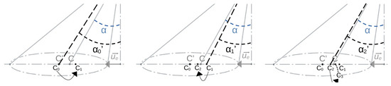
Figure 4.
Iterative process for computing C. In every iteration (from left to right), a new estimation of and is computed. The unitary vector define the line containing , C and O.
Hence, an iterative algorithm named Precise Center Location (PCL, Algorithm 1) is proposed to numerically compute C. After computing , the algorithm starts with C estimated as , and iteratively re-estimates its value until convergence.
| Algorithm 1 Precise Center Location (PCL) |
|
Several practical considerations need to be taken into account. On the one hand, and C are expressed in real-world units with a center on the principal point of the camera sensor (O). Thus, the intrinsic camera parameters (sensor resolution, pixel size, optical distortion, ⋯) must be known to convert the image pixel coordinates to real-world units. It is important to have a good model of the camera’s optical distortion [15,16] to correct pixel positions before to converting them to real-world units.
In addition, an estimation of the work distance must be provided. This value can be estimated fairly in scenarios where the camera positions are fixed and can be refined on each iteration for iterative calibration algorithms (see Section 3.3).
3. Experiments
To test our algorithm and to present a case study, a real 3D capture device was used. The ZG3D device is a 3D scanner (see Figure 5) made up of 16 cameras pointing to its center. These cameras capture falling objects from different points of view, and a specific software program reconstructs them using shape-from-silhouette techniques ([2,17]).
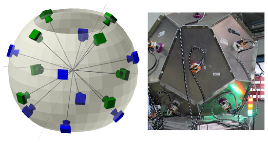
Figure 5.
ZG3D capture device. Camera distribution (left). Actual device (right). The objects are captured as they fall through the device.
The cameras on this device must be calibrated accurately to obtain a precise reconstruction. This is done by means of a multiview calibration algorithm [3] that uses a calibrated token consisting of two spheres of different sizes connected by a narrow cylinder (see Figure 6). The calibration process presented in [3] is fed with several captures of the token, where the sphere center projections should be located and used as input for the algorithm.

Figure 6.
The calibration token consisted of two spheres of different diameters connected by a narrow cylinder (left). The center projections of both spheres were located on the images (right).
The ZG3D device has 16 XCG-CG510 (Sony Corporation) cameras, with a sensor resolution of pixels, a pixel size of 3, 45 m and a 25 mm focal length lens. They were 550 mm from the center of the device, where the objects were captured.
The token is a calibrated item composed by two spheres of diameters 43.5 mm and 26.1 mm that are 65.25 mm apart. They were connected by a cylinder of 8 mm in diameter.
The experiments were performed using synthetic and real captures from the ZG3D device. Each capture consisted of 16 images (one per camera; see Figure 7) of the calibration token. For the synthetic captures, a CAD model of the ZG3D device and the calibration token was employed, and the images were obtained using z-buffer techniques [18]. In both scenarios, five capture datasets were created, each containing 20 captures of the calibration token in random positions.
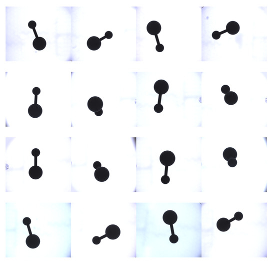
Figure 7.
An example of capture. On each capture, 16 images were obtained in the device.
In this section, a test that verifies the precision of the PCL algorithm is first presented. Hereafter, the method to estimate the error map for a specific scenario is shown—in our case, for the ZG3D device. Finally, the performance of the calibration algorithm is tested when the sphere center projection is corrected using the PCL algorithm.
3.1. Precision Test
Synthetic datasets were employed to check the precision of the PCL algorithm. During the dataset construction, the exact position and orientation of the token were known because a CAD model was used, thus allowing us to compute the exact sphere center projections on each image. These values, representing the ground truth, were compared to the values obtained using the silhouette center algorithm employed in [3] (see Figure 6) with and without the proposed correction. A total of images constituted the synthetic dataset, each containing two spheres. After eliminating images with occlusions and with cropped tokens on the borders, a total of 1134 images were available.
An error value is defined as the Euclidean distance between the real projected center and the computed point in the image. Figure 8 shows the error distributions for the calculated sphere center projection points on both spheres. As expected, the large sphere has a larger error for the uncorrected points; however, after correction, both spheres have similar distributions and present a minimal error. These small errors can be caused by errors in the blob center detection algorithm, but are probably caused by the estimation of the work distance (W) used. A value of 550 mm was employed, defined by the distance between the cameras and the center of the capture area in the device. However, small deviations in the token falling path and/or its variable position result in slightly different values for each camera.
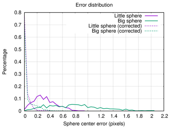
Figure 8.
Distribution error of sphere center calculations for both calibration token spheres. The graph shows the estimation error before and after applying the proposed sphere center correction algorithm with the context parameters.
On the other hand, the iterative algorithm converges very quickly, requiring only a few iterations (less than 5) to achieve a precision () of in this case study.
3.2. Error Estimation
The developed algorithm can be employed to analyze the error when computing the sphere center projection as the sphere blob center in images—for example, in cases where computer power is limited and it is of interest to avoid executing unnecessary code.
Figure 9 shows the error maps obtained for both token spheres depending on their position on the image in the ZG3D device. In this case, an error range of and pixels are obtained for the small and the large spheres, respectively. These ranges are consistent with the results presented in Figure 8. Whether these errors are acceptable or not depends on each application. Regarding our case study, this point will be discussed in the next section.
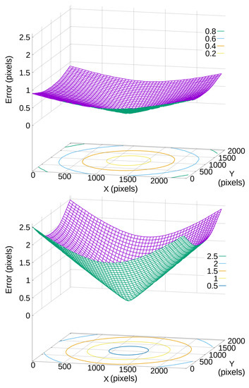
Figure 9.
The error between the blob center and the sphere center projection with data: mm, mm, sphere diameter mm (top) and mm (bottom) on an image (, pixel size = m). The bottom of the curve represents a null error.
Capture system parameters (F, W, D, ⋯) can be explored so that error maps can be obtained to set them to the desired error range and/or to decide if the PCL algorithm correction is needed. Figure 10 shows the maximal error obtained (which appears when the sphere is in an image corner) for the ZG3D cameras while varying their focal length (F) and working distance (W) with spheres of different diameters (D). These maps can help to configure these parameters in the design phase.
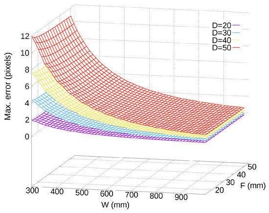
Figure 10.
Maximal error on the image ( pixels, m pixel size) for different values of the work distance (W), focal length (F) and the sphere diameter (D).
3.3. Calibration Performance Tests
The impact of sphere center projection correction in the ZG3D calibration algorithm [3] is tested in this section. The calibration algorithm uses as input the intrinsic camera parameters computed separately for each camera, a coarse initialization of the extrinsic parameters, the token dimensions and the sphere center projections () obtained from the silhouettes of a set of token captures.
As shown in Figure 11, the algorithm uses the sphere center projections of each capture to compute the epipolar lines using the estimated intrinsic and extrinsic parameters of each camera. These lines are then used to triangulate the sphere centers in the 3D space (more details in [3]) and a correspondence between camera points and 3D points can be built for each camera using several sphere captures. With this information, the extrinsic parameters are recalibrated using a gradient descent algorithm and a new iteration is started with the recalibrated extrinsic parameters until convergence.
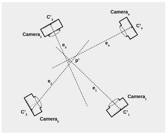
Figure 11.
Each point is the computed center projection of a target sphere captured with camera i; an epipolar line can be obtained for each point–camera pair. With the epilopar lines, the point (the estimated sphere center in the 3D space) can be obtained by triangulation. A more precise estimation of point implies a more precise estimation.
Because this algorithm estimates the sphere centers in the 3D space, and because an estimation of the camera positions exists in each iteration, the working distances (W) can be estimated and conveniently used in the PCL algorithm. The PCL algorithm was then incorporated into the calibration process to produce more accurate epipolar lines; thus, the triangulation process is more precise.
To compare the calibration results, two values were employed; on the one hand, we used the quadratic error distance between the calibrated and real camera positions. Obviously, this value can only be computed for the virtual datasets. On the other hand, the dispersion (standard deviation) of the token size estimated by each camera after calibration was calculated. This size is computed as the distance between their sphere centers, which theoretically should be mm. This measure is proposed because it gives a good estimation of the calibration quality [3].
Three experiments were performed employing the virtual datasets:
- using the exact sphere center projections (C) from the CAD models;
- using the estimated projections from capture images () without PCL;
- using the estimated projections from capture images (), including PCL on the calibration algorithm.
Moreover, two more experiments were performed employing the real datasets:
- using the estimated projections from capture images () without PCL;
- using the estimated projections from capture images (), including PCL on the calibration algorithm.
In each experiment, five executions of the calibration algorithm (one per dataset) were performed and the results were averaged. Table 1 and Table 2 show the results obtained for each case. The experiment with the exact projections shows that the calibration algorithm can achieve the exact calibration in this case. If the estimated projections are used, activating the PCL algorithm offers a significantly lower value in both the error distance and dispersion, giving results close to the exact values for the virtual datasets.

Table 1.
Token size dispersion after calibration on both virtual and real datasets (in mm).
Table 2.
Mean quadratic camera error distances between the calibrated and CAD model cameras using virtual datasets (in mm).
By comparison, the results on real datasets are not as significant as those for the virtual datasets, but still provide an interesting improvement. In this case, other error sources probably have a significant effect on the quality of the calibration (real image artifacts, inaccuracies in the lens distortion model of the intrinsic parameters, etc.).
4. Conclusions
This work presents a simple numerical method to obtain the exact sphere center projection on an image using the Precision Center Location (PCL) algorithm. It is based on the correction of the centroid of the sphere silhouette projection on the image. No ellipse fitting or area estimations are needed, as in other mentioned works [1,4,9,11,12], minimizing the errors derived from edge detection or image segmentation algorithms. These errors are derived from poorly illuminated scenes or from systems with camera lens configurations with significant optical diffraction, or dispersion, where blurry contours can appear.
The PCL algorithm is fast and accurate, as shown in Section 3.1. Its implementation is very straightforward and intuitive, avoiding the complex formulations employed by other methods. It can be programmed easily.
In addition, the sphere center projection estimated as the silhouette centroid on images could be accurate enough depending the camera/system configuration—for example, if the ratio is high enough, or simply because the system does not require extreme precision. In these cases, the algorithm can be used to calculate the errors in the estimation and to decide if a more elaborate solution is needed. This can be useful to save computer resources, simplify software, etc.
Finally, in Section 3.3, a case study is presented to illustrate the integration of this algorithm in a multi-view camera calibration algorithm using spheres as calibration targets. The integration was straightforward and the sphere center projections were corrected on each iteration of the PCL algorithm. With this correction, the calibration accuracy obtained was improved. On the virtual dataset, the error estimators were significantly reduced, showing the importance of an exact estimation of the sphere center projection if high accuracy is needed and every error source should be analyzed. On the real dataset, the improvement was smaller; nevertheless, other error sources more difficult to eliminate or to model (real image artifacts, small inaccuracies in the distortion camera model, etc.) should be taken into account.
Author Contributions
Conceptualization, A.J.P.; methodology, A.J.P. and J.-C.P.-C.; software, A.J.P. and J.-L.G.; writing—original draft, A.J.P.; writing—review and editing, J.P.-S. and A.J.P. All authors have read and agreed to the published version of the manuscript.
Funding
This work was partially funded by Generalitat Valenciana through IVACE (Valencian Institute of Business Competitiveness) distributed nominatively to Valencian technological innovation centres under project expedient IMAMCN/2021/1.
Institutional Review Board Statement
Not applicable.
Informed Consent Statement
Not applicable.
Data Availability Statement
All data has been presented in the main text.
Conflicts of Interest
The authors declare no conflict of interest.
References
- Penne, R.; Ribbens, B.; Roios, P. An Exact Robust Method to Localize a Known Sphere by Means of One Image. Int. J. Comput. Vis. 2019, 127, 1012–1024. [Google Scholar] [CrossRef]
- Perez-Cortes, J.C.; Perez, A.J.; Saez-Barona, S.; Guardiola, J.L.; Salvador, I. A System for In-Line 3D Inspection without Hidden Surfaces. Sensors 2018, 18, 2993. [Google Scholar] [CrossRef] [PubMed] [Green Version]
- Perez, A.J.; Perez-Cortes, J.C.; Guardiola, J.L. Simple and precise multi-view camera calibration for 3D reconstruction. Comput. Ind. 2020, 123, 103256. [Google Scholar] [CrossRef]
- Agrawal, M.; Davis, L.S. Camera calibration using spheres: A semi-definite programming approach. In Proceedings of the Ninth IEEE International Conference on Computer Vision, Nice, France, 13–16 October 2003; pp. 782–789. [Google Scholar]
- Safaee-Rad, R.; Tchoukanov, I.; Smith, K.; Benhabib, B. Three-dimensional location estimation of circular features for machine vision. IEEE Trans. Robot. Autom. 1992, 8, 624–640. [Google Scholar] [CrossRef] [Green Version]
- Huang, H.; Zhang, H.; Cheung, Y.-m. The common self-polar triangle of concentric circles and its application to camera calibration. In Proceedings of the 2015 IEEE Conference on Computer Vision and Pattern Recognition (CVPR), Boston, MA, USA, 7–12 June 2015; pp. 4065–4072. [Google Scholar]
- Matsuoka, R.; Sone, M.; Sudo, N.; Yokotsuka, H.; Shirai, N. A Study on Location Measurement of Circular Target on Oblique Image. Opt. 3-D Meas. Tech. IX 2009, I, 312–317. [Google Scholar]
- Matsuoka, R.; Shirai, N.; Asonuma, K.; Sone, M.; Sudo, N.; Yokotsuka, H. Measurement Accuracy of Center Location of a Circle by Centroid Method. In Photogrammetric Image Analysis; Stilla, U., Rottensteiner, F., Mayer, H., Jutzi, B., Butenuth, M., Eds.; Springer: Berlin/Heidelberg, Germany, 2011; pp. 297–308. [Google Scholar]
- Matsuoka, R.; Maruyama, S. Eccentricity on an image caused by projection of a circle and a sphere. ISPRS Ann. Photogramm. Remote Sens. Spat. Inf. Sci. 2016, III-5, 19–26. [Google Scholar] [CrossRef] [Green Version]
- Luhmann, T. Eccentricity in images of circular and spherical targets and its impact on spatial intersection. Photogramm. Rec. 2014, 29, 417–433. [Google Scholar] [CrossRef]
- Shiu, Y.C.; Ahmad, S. 3D location of circular and spherical features by monocular model-based vision. In Proceedings of the IEEE International Conference on Systems, Man and Cybernetics, Cambridge, MA, USA, 14–17 November 1989; pp. 576–581. [Google Scholar]
- Guan, J.; Deboeverie, F.; Slembrouck, M.; Van Haerenborgh, D.; Van Cauwelaert, D.; Veelaert, P.; Philips, W. Extrinsic Calibration of Camera Networks Using a Sphere. Sensors 2015, 15, 18985–19005. [Google Scholar] [CrossRef] [PubMed] [Green Version]
- Faugeras, O. Three-Dimensional Computer Vision: A Geometric Viewpoint; MIT Press: Cambridge, MA, USA, 1993. [Google Scholar]
- Anton, H. Elementary Linear Algebra; John Wiley and Sons: Hoboken, NJ, USA, 1994. [Google Scholar]
- Zhang, Z. A Flexible New Technique for Camera Calibration. IEEE Trans. Pattern Anal. Mach. Intell. 2000, 22, 1330–1334. [Google Scholar] [CrossRef] [Green Version]
- Wang, J.; Shi, F.; Zhang, J.; Liu, Y. A new calibration model of camera lens distortion. Pattern Recognit. 2008, 41, 607–615. [Google Scholar] [CrossRef]
- Dyer, C.R. Volumetric Scene Reconstruction From Multiple Views. In Foundations of Image Understanding; Springer: Boston, MA, USA, 2001; pp. 469–489. [Google Scholar]
- Karinthi, R. VII.6—Accurate Z-Buffer Rendering. In Graphics Gems V; Paeth, A.W., Ed.; Academic Press: Boston, MA, USA, 1995; pp. 398–399. [Google Scholar] [CrossRef]
Publisher’s Note: MDPI stays neutral with regard to jurisdictional claims in published maps and institutional affiliations. |
© 2022 by the authors. Licensee MDPI, Basel, Switzerland. This article is an open access article distributed under the terms and conditions of the Creative Commons Attribution (CC BY) license (https://creativecommons.org/licenses/by/4.0/).