3. Multidimensional Scaling (MDS) Background
This work focuses on FTM exchanges between fixed points. In this context, Wi-Fi access points and other static devices (e.g., digital signage) can be configured to play the role of ISTAs and RSTAs, alternating between one and the other and ranging to one another over time. As the points are fixed, and as each ranging burst takes a few hundreds of milliseconds (e.g., a burst of 30 exchanges would consume about 250 ms in good RF conditions), a large number of samples can be taken (e.g., a burst per minute represents 43,200 samples per 24-hour period). This flexibility allows for obtaining ranges between pairs far apart, and for which only a few exchanges succeed. From all exchanges, only the best (typically smallest) distance is retained, as will be seen later. The output of these FTM measurements is a network of nodes, among which nodes have a known position.
The measured distance between these nodes can be organized in a matrix that we will note . Conceptually, the set is similar to any other noisy Euclidean Distance Matrix (EDM). The set contains an exhaustive table of distances between points taken by pairs from a list of points x in N dimensions and for any point . Each point is labelled ordinally, hence each row or column of an EDM, i.e., , individually addresses all the points in the list. The main task of the experimenter is then to find the dimension N and construct a matrix of distances that on one hand best resolves the noise (which causes inconsistencies between the various measured pairs), and on the the other hand is closest to the real physical distances between points, called ground truth, and which matrix is noted D. Such task is one main object of Multidimensional Scaling (MDS).
MDS draws its origin from psychometrics and psychophysics. MDS considers a set of n elements and attempts to evaluate similarities or dissimilarities between them. These properties are measured by organizing the set elements in a multi-dimensional geometric object where the properties under evaluation are represented by distances between the various elements. MDS thus surfaces geometrical proximity between elements displaying similar properties in some dimension of an space. The properties can be qualitative (non-metric MDS, nMDS), where proximity may be a similarity ranking value, or quantitative (metric MDS, mMDS), where distances are expressed. This paper will focus on mMDS.
Two main principles lie at the heart of mMDS: the idea that distances can be converted to coordinates, and the idea that during such process dimensions can be evaluated. The coordinate matrix
X is an
object, where each row
i expresses the coordinate of the point
i in
N dimensions. Applying the squared Euclidean distance equation to all points
i and
j in
X (Euclidean distance
, which we write
for simplicity) allows for an interesting observation:
Applying this equation to the distance matrix
D, noting
the squared distance matrix for all
,
c an
column vector of all ones,
the column
a of matrix X, noting
e a vector that has elements
, and writing
the transpose of any matrix
A, the equation becomes:
This observation is interesting, in particular because it can be verified that the diagonal elements of are , i.e., the elements of e. Thus, from X, it is quite simple to compute the distance matrix D. However, mMDS usually starts from the distance matrix D, and attempts to find the position matrix X, or its closest expression U. This is also FTM approach, that starts from distances and attempt to deduce location. As such, mMDS is directly applicable to FTM.
Such reverse process is possible, because one can observe that D, being the sum of scalar products of consistent dimensions, is square and symmetric (and with only positive values). This observation is intuitively obvious, as D expresses the distance between all point pairs, and thus each point represents one row and one column in D. These properties are very useful, because a matrix with such structure can be transformed in multiple ways, in particular through the process of eigendecomposition, by which the square, positive and symmetric matrix B of size can be decomposed as follows: , where matrix Q is orthonormal (i.e., Q is invertible and we have ) and is a diagonal matrix such that . Values of are the eigenvalues of B. Eigenvalues are useful to find eigenvectors, which are sets of individual non-null vectors that satisfy the property: , i.e., the direction of does not change when transformed by B.
In the context of MDS, this decomposition is in fact an extension of general properties of Hermitian matrices, for which real and symmetric matrices are a special case. A square matrix B is Hermitian if it is equal to its complex conjugate transpose , i.e., .
In terms of the matrix elements, such equality means that . A symmetric MDS matrix in obviously respects this property, and has the associated property that the matrix can be expressed as the product of two matrices, formed from one matrix U and its transpose , thus . Because this expression can be found, B is said to be positive semi-definite (definite because it can be classified as positive or negative, positive because the determinant of every principal submatrix is positive, and positive semi-definite if 0 is also a possible solution). A positive semi-definite matrix has non-negative eigenvalues.
This last property is important for mMDS and for the FTM case addressed in this paper. As
can be rewritten as
, it follows that non-null eigenvectors are orthogonal. As such, the number of non-null eigenvalues is equal to the rank of the matrix, i.e., its dimension. This dimension is understood as the dimension of the object studied by MDS. With FTM, this outcome determines if the graph formed by APs ranging once another is in 2 dimensions (e.g., all APs on the same floor, at ceiling level) or in 3 dimension (e.g., APs on different floors). In a real world experiment,
B is derived from
and is therefore noisy. But one interpretation of the eigendecomposition of
B is that it approximates
B by a matrix of lower rank
k, where
k is the number of non-null eigenvalues, which can then represent the real dimensions of the space where
B was produced. This is because, if
is the
i-th column vector of
Q (and therefore
the
i-th row vector of
), then
can be written as:
Therefore, if
eigenvalues are 0, so is their individual
product, and an image of
B can be written as:
C and B have the same non-null eigenvectors, i.e., C is a submatrix of B restricted to the dimension of B’s non-null eigenvalues. In noisy matrices, where distances are approximated, it is common that all eigenvalues will be non-null. However, the decomposition should expose large eigenvalues (i.e., values that have a large effect on found eigenvectors) and comparatively small eigenvalues (i.e., values that tend to reduce eigenvectors close to the null vector). Small eigenvalues are therefore ignored and considered to be null values that appear as non-zero because of the matrix noise.
An additional property listed above is that positive semi-definite matrices only have non-negative eigenvalues. In the context of MDS, this is all the more logical, as each eigenvector expresses one dimension of the space. However, noisy matrices may practically also surface some negative eigenvalues. The common practice is to ignore them for rank estimation, and consider them as undesirable but unavoidable result of noise. We will apply the same principles for measurements obtained with FTM. However, it is clear that the presence of many and/or large negative eigenvalues is either a sign that the geometric object studied under the MDS process is not Euclidian, or that noise is large, thus limiting the possibilities of using the matrix directly, without further manipulation.
Therefore, if from Equation (
3) above, one defines
, then an eigendecomposition of
B can be performed as
. As scalar product matrices are symmetric and have non-negative eigenvalues, one can define
as a diagonal matrix with diagonal elements
. From this, one can write
The coordinates in U differ from those in X, which means that they are expressed relative to different coordinate systems. However, they represent the geometric object studied by MDS with the same dimensions and scale. Thus, a rotation can be found to transform one into the other.
With these transformations, mMDS can convert a distance matrix into a coordinate matrix, while estimating the space dimension in the process. Thus, classical mMDS starts by computing, from all measured distances, the squared distance matrix
. The measured distance matrix
is also commonly called, in MDS in general, the proximity matrix, or the similarity matrix. Next, a matrix called the
J is computed, that is in the form
where
c is an
column vector of all ones. Such matrix is a set of weights which column or row-wise sum is twice the mean of the number of entries
n. This matrix has useful properties described in [
18]. In particular, applied to
, it allows the determination of the centered matrix
, which is a transformation of
around the mean positions of
. This can be seen as follows:
By transposing
J into the expression, it can easily be seen that, as
and
:
At this point, the distance matrix is centered. This phase has a particular importance for the method proposed in this paper, because we will see below that its direct effect is to dilute the noise of one pair into the measurements reported by other pairs, thus causing mMDS to fail in highly asymmetric measurements like FTM. mMDS then computes the eigendecomposition of . Next, the experimenter has the possibility to decide of the dimensions of the projection space ( or in our case, but the dimension can be any in mMDS). This can be done by arbitrarily choosing the m largest eigenvalues and their corresponding eigenvectors of B. This choice is useful when the experimenter decides to project the distance matrix into m dimensions, and has decided of what value m should be. Alternatively, the experimenter can observe all eigenvalues in B and decide that the dimension space matches all m large positive eigenvalues in B, ignoring the (comparatively) small positive eigenvalues, along with the null and negative eigenvalues as detailed in the previous section.
Then, if we write the matrix of these m largest positive eigenvalues, and the first m columns in Q (thus the matrix of eigenvalues matching the dimensions decided by the experimenter), the coordinate matrix is determined to be .
5. Materials and Methods
5.1. First Component: Wall Remover-Minimization of Asymmetric Errors
One first contribution of this paper is a method to reduce dilation asymmetry. Space dimension is resolved using other techniques (e.g., RSSI-based), and
Section 6 will provide an example. Once the dimension space has been reduced to
and only sensors on the same floor, we want to reduce the dilation asymmetry.
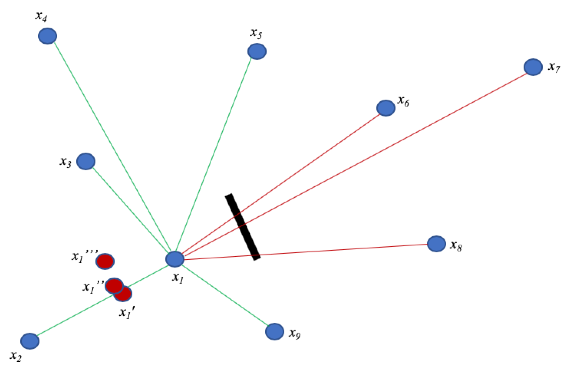
Figure 1 illustrates a typical asymmetry scenario. In this simplified representation, a strong obstacle appears between the sensor
and sensors
and
, causing the distances
,
and
to be appear as
,
and
respectively. At the same time, supposing that the system is calibrated properly and LoS conditions exist elsewhere, the obstacle does not affect distance measurements between
and
and
, that are all approximated along the same linear dilation factor
k.
In such case, using a centering technique to average the error may make sense algebraically, but not geometrically. Finding a method to reduce the error while detecting its directionality is therefore highly desirable. Luckily, geometry provides great methods to this mean, that only have the inconvenience of requiring multiple comparisons. Such process may be difficult when performing individual and mobile station ranging, but becomes accessible when all sensors are static. When implemented in a learning machine, this method can be implemented at scale and reduce the distance error only when it is directional, thus outputting a matrix
which
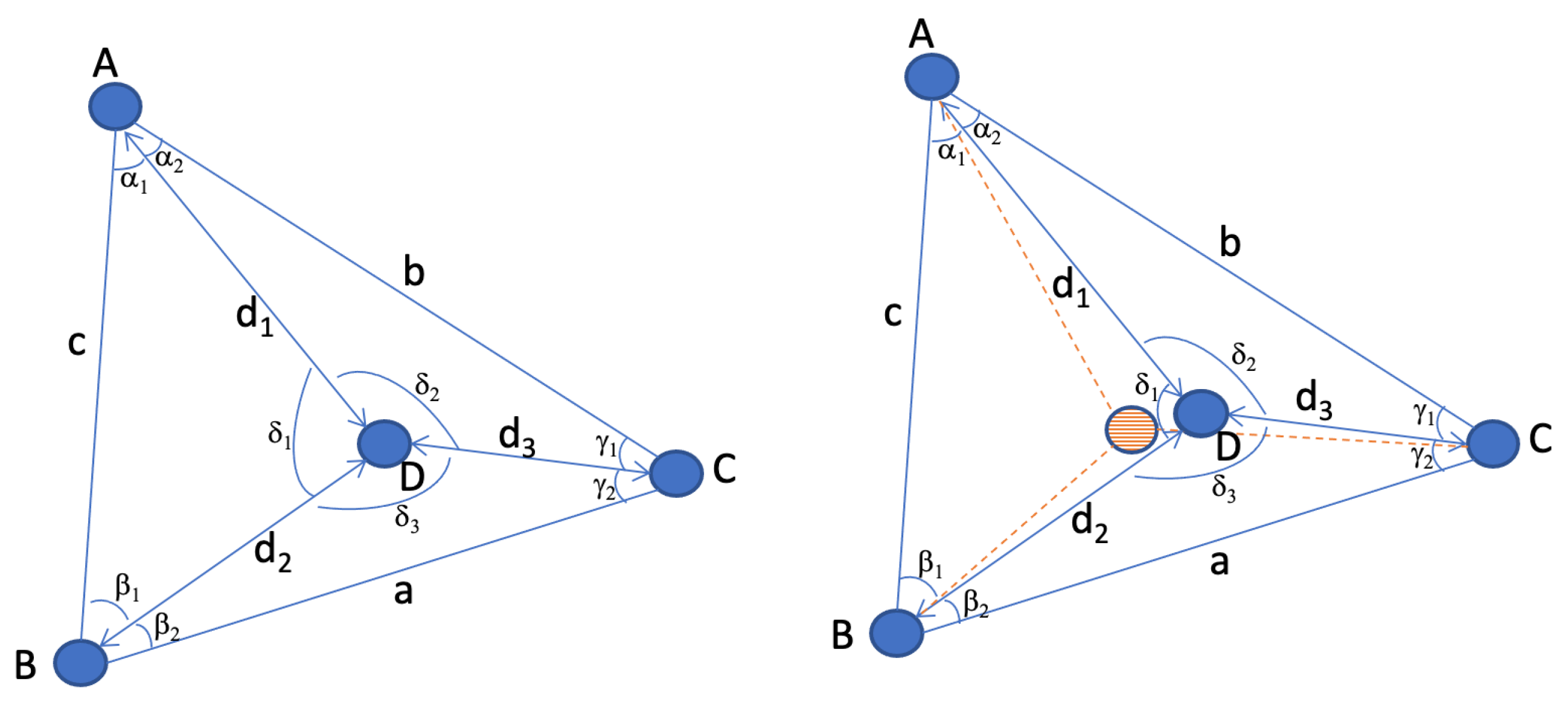
k factor is closer to uniformity. It should be noted that the purpose of such method should not be to fully solve the MDS problem, as some pair-distances are usually not known, and the method has a limited scope (i.e., it cannot assess some of the pairs, as will be seen below). However, in many cases, sensors can be found that display interesting properties displayed on the left part of
Figure 3. In this scenario, 3 sensors
and
are selected that form a triangle. The triangle represented in the left part of
Figure 3 is scalene, but the same principle applies to any triangle. A fourth sensor
is found which distance to
and
is less than
or
, thus placing
within the triangle formed by
.
A natural property of such configuration is that
and, in any of the triangles
or
, one side can be expressed as a combination of the other two and of its opposite angle. For example,
in
can be expressed as:
The above easily allows us to find
and can also be used to determine angles from known distances, for example
, knowing that:
Therefore, angles and missing distances can be found from known distances. In an ideal world, properties (
20) and (
21) are verified for each observed triangle (
and (
)). In a noisy measurement scenario, inconsistencies are found. For example, an evaluation of the triangle
may be consistent with the left side of
Figure 3, but an evaluation of triangle
may position
in the hashed representation
of the right part of
Figure 3. It would be algebraically tempting to resolve
as the middle point between both possibilities (mean error). However, this is not the best solution. In
Figure 3 simplified example, the most probable reason for the inconsistency is the presence of an obstacle or reflection source between
and
. If all distances are approximations, some of them being close to the ground truth and some of them displaying a larger
k factor, a congruent representation of such asymmetry is that
k is larger for
than it is for the other segments. Quite obviously, other possibilities can be found. For example, in the individual triangle
, it is possible that
k is larger for the segments
than it is for segments
and
. However, as
is compared to other segments and the same anomaly repeats, the probability that the cause is an excessive stretch on
increases.
As the same measurements are performed for more points, the same type of inconsistency appears for other segments. Thus an efficient resolution method is to identify these inconsistencies, determine that the distance surfaced for the affected segment is larger than a LoS measurement would estimate, then attempt to individually and progressively reduce the distance (by a local contraction factor that we call ), until inconsistencies are reduced to an acceptable level (that we call ).
Thus, formally, a learning machine that we call a geometric Wall Remover engine, is fed with all possible individual distances in the matrix, and compares all possible iterations of sensors forming a triangle and also containing another sensor. Distance matrices do not have orientation properties. When considering for example, can be found on either side of segment , and the solution can also be a triangle in any orientation. However, adding a fourth point (), which distance to is evaluated, can constrain within the triangle. As the evaluation proceeds iteratively throughout all possible triangles that can be formed from the distance matrix, the system first learns to place the sensors relative to each other. The resulting sensor constellation can have globally any orientation, but the contributing points partially appear in their correct relative position.
Then, each time a scenario matching the right side of
Figure 3 is found, the algorithm learns the asymmetry and increases the weight
w of the probability
p that the matching segment (
in this example) has a dilated
factor (cf. Algorithm 1). As a segment may be evaluated against many others, its
w may accordingly increase several times at each run. The algorithm starts by evaluating the largest found triangles first (sorted distances from large to small), because they are the most likely to be edge sensors. This order is important, because in
Figure 3 example, a stretched
value may cause
to be graphed on the right side of segment
, and thus outside of
. This risk is mitigated if multiple other triangles within
can also be evaluated. An example is depicted by
Figure 4. In this simplified representation (not all segments are marked), the position of
is constrained by first evaluating
and
against
and
. This evaluation allows the system to surface the high probability of the stretch of segment
, suggesting that
should be closer to
than the measured distance
suggests, but not to the point of being on the right side of
. The system can similarly detect a stretch between points
and
(but not between
and
or
and
).
| Algorithm 1: Wall Remover Algorithm |
Input : : learning rate
: acceptable error range |
| Output: optimized |
 |
At the end of the first training iteration, the system outputs a sorted list of segments with the largest stretch probabilities (largest w and therefore largest p). The system then picks that segment with that largest stretch, and attempts to reduce its stretch by proposing a contraction of the distance by an individual factor. The factor can be a step increment (similar to other machine learning algorithms learning rate logic) or can be proportional to the stretch probability. After applying the contraction, the system runs the next iteration, evaluating progressively from outside in, each possible triangle combination. The system then recomputes the stretch probabilities and proposes the next contraction cycle. In other words, by examining all possible triangle combinations, the system learns stretched segments and attempts to reduce the stretch by progressively applying contractions until inner neighboring angles become as coherent as possible, i.e., until the largest stretch is within a (configurable) acceptable range from the others.
This method has the merit of surfacing points internal to the constellation that display large k factors, but is also limited in scope and intent. In particular, it cannot determine large k factors for outer segments, as the matching points cannot be inserted within triangles formed by other points. However, its purpose is to limit the effect on measurements of asymmetric obstacles or sources of reflection.
5.2. Second Component: Iterative Algebro-Geometric EDM Resolution
The output of the wall remover method is a matrix with lower variability to the dilation factor k, but the method does not provide a solution for an incomplete and noisy EDM. Such reduction still limits the asymmetry of the noise, which will therefore also limit the error and its locality when resolving the EDM, as will be shown below. Noise reduction can be used on its own as a preparatory step to classical EDM resolution techniques. It can also be used in combination with the iterative method we propose in this section, although the iterative method has the advantage of also surfacing dilation asymmetries, and thus could be used directly (without prior dilation reduction). Combined together, these two techniques provide better result than standard EDM techniques.
EDM resolution can borrow from many techniques, which address two contiguous but discrete problems: matrix completion and matrix resolution. In most cases, the measured distance matrix has missing entries, indicating unobserved distances. In the case of FTM, these missing distances represent out-of-range pairs (e.g., sensors at opposite positions on a floor or separated by a strong obstacle, and that cannot detect each other). A first task is to complete the matrix, by estimating these missing distances. Once the matrix contains non-zero numerical values (except for the diagonal, which is always the distance and therefore always 0), the next task is to reconcile the inconsistencies and find the best possible distance combination.
Several methods solve both problems with the same algorithm and [
21] provides a description of the most popular implementations. We propose a geometric method, that we call Iterative Algebro-Geometric EDM resolver (Algorithm 2), which uses partial matrix resolution as a way to project sensor positions geometrically onto a
plane, then a mean cluster error method to identify individual points in individual sets that display large asymmetric distortions (and should therefore be voted out from the matrix reconstruction). By iteratively attempting to determine and graph the position of all possible matrices for which point distances are available, then by discarding the poor (point pairs, matrices) performers and recomputing positions without them, then by finding the position of the resulting position clusters, the system reduces asymmetries and computes the most likely position for each sensor.
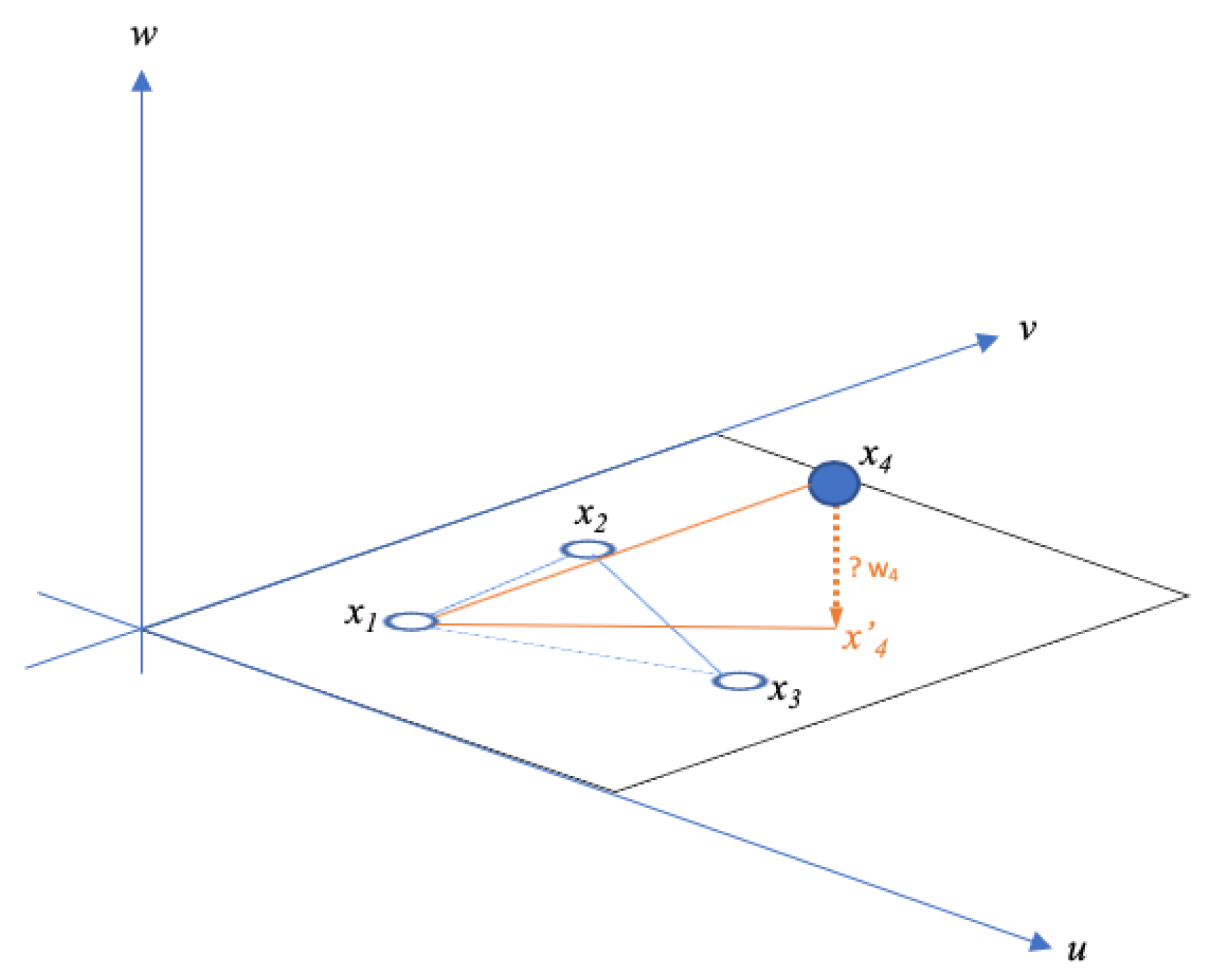
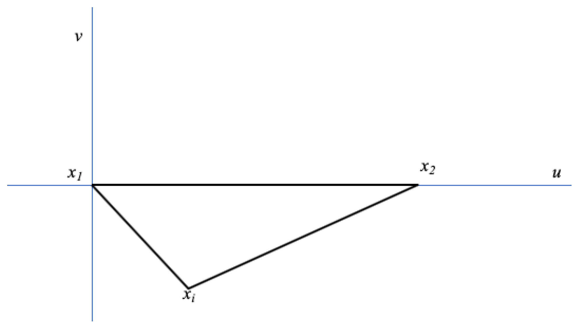
We want to graph the position of each point in the sub-matrix. A pivot
is chosen iteratively in
. In the first iteration,
, then
in the second iteration, and
in the last iteration. For each iteration,
is set as the origin, and
. An example is displayed in
Figure 5. The next point
in the matrix (
) is iteratively set along the
x-axis, and
. If
, then the position of each other point
of the set
is found using standard triangular formula illustrated by the points in
Figure 5 and where:
and
| Algorithm 2: Iterative algebro-geometric EDM resolution algorithm |
| Input: |
 |
Formally, the measured distance matrix
of
n sensor distances is separated in sub-matrices. Each sub-matrix
contains
points for which inter-distances were measured, so that:
Such formula fixes the position of above the u-axis (because is always positive). This may be ’s correct position in the sensor constellation in some cases, but can also result in an incorrect representation as soon as the next point is introduced in the graph. A simple determination of the respective positions of and can be made by evaluating their distances, as in the wall remover method. In short, if , then and are on opposite sides of the u-axis and becomes .
As the process completes within the first matrix, the position of
m points are determined using the first pair of points
and
as the reference. In the next iteration,
is kept but
changes from
to
. Algebraically, the first iteration determines the positions based on the pairwise distances expressed in the first 2 columns of the distance matrix, while the second iteration determines the positions based on the pairwise distances expressed in the first and third columns. Both results overlap for the first 3 points
and
, but not for the subsequent points. This can be easily understood with an example. Recall that for any pair of points
i and
j,
. Using
as a representation of both
and
, and the following small matrix of 5 points as an example:
The first iteration ignores and that are represented in the second iteration (but the second iteration does not represent or ).
As in the second iteration
is used as a reference point for the x axis, the geometrical representations of the first and the second iterations are misaligned. However,
is at the origin in both cases, and
is represented in both graphs (we note them
and
). Using Equation (
22), finding the angle
formed by the points
is straightforward, and projecting the second matrix into the same coordinate reference as the first matrix is a simple rotation of the second matrix, defined by
T as:
In the subsequent iterations,
ceases to be at the origin. Depending on the sub-matrix and the iteration,
may or may not be in the new matrix. However, 2 points
and
can always be found that are common to both the previous matrix
and the next matrix
. Projecting
into the same coordinate reference as
is here again trivial, by first moving the coordinates of each point found from
by
and
then perform a rotation using Equation (
22). These operations are conducted iteratively. As measured distances are noisy, for each point represented in
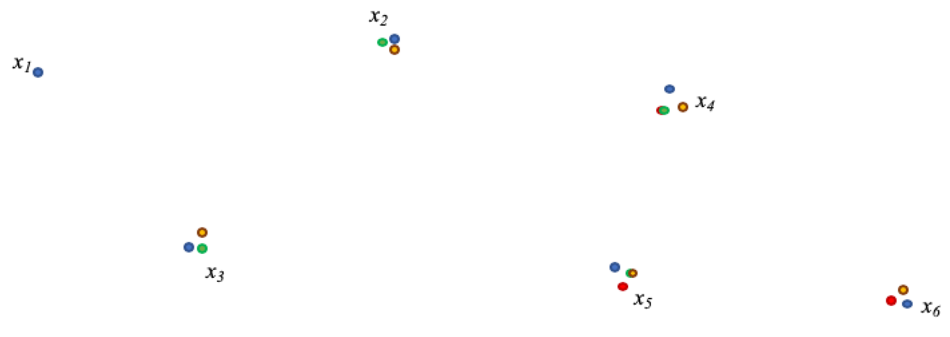
, different coordinates appear at the end of each iteration, thus surfacing for each point a cluster of computed coordinates.
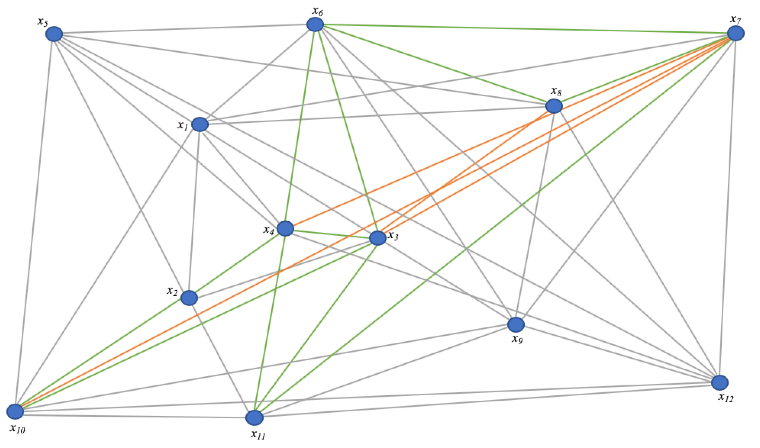
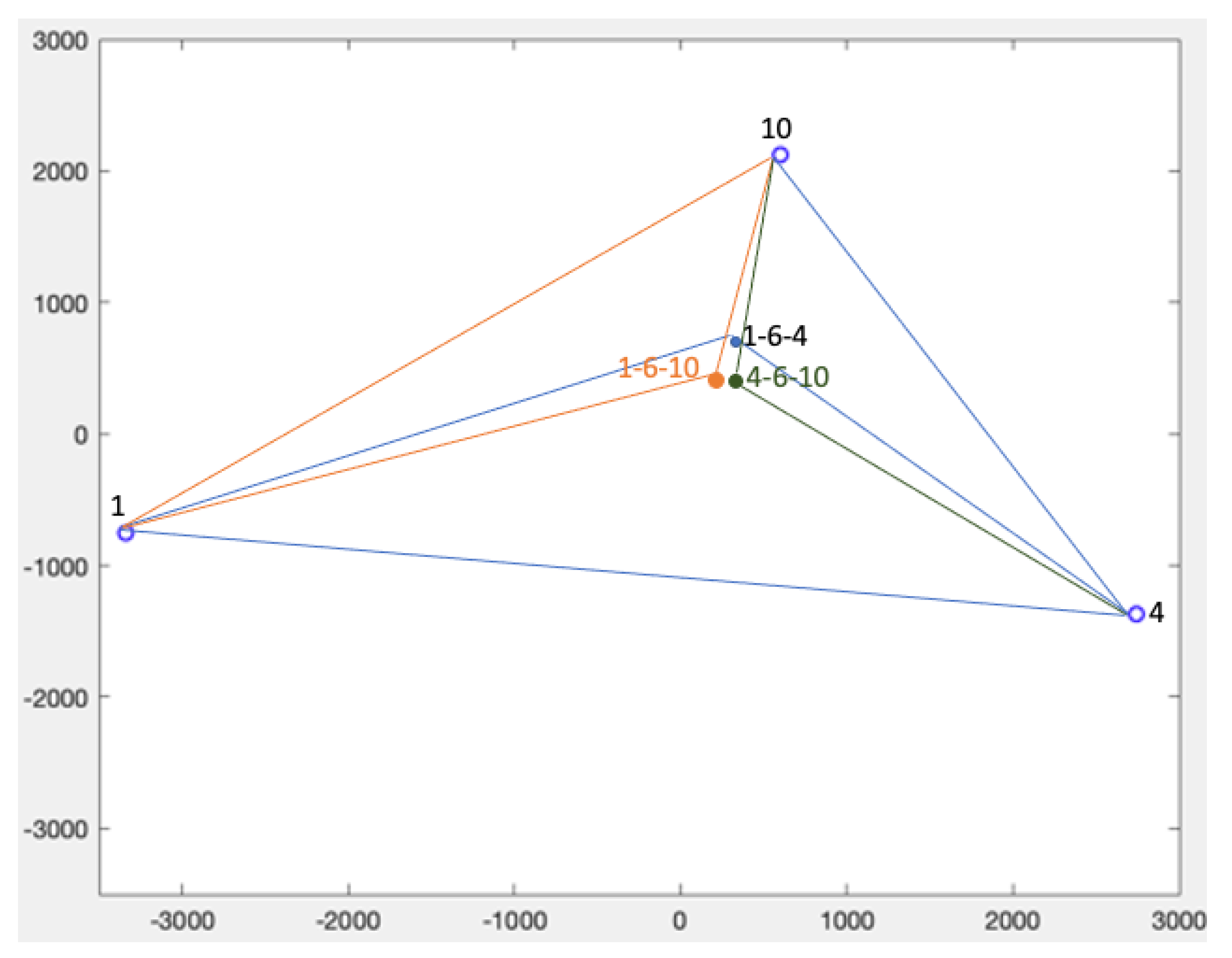
Figure 6 represents this outcome after 4 iterations over a 5-point matrix and
fixed about the first point.
The effect of projection and rotation makes that the red and green points are overlapping in
, and the green and orange point are overlapping in
. The choice to determine which points should be used to project
onto
is sequentially obvious, but arbitrary otherwise. In the example displayed in
Figure 6,
instead of
could have been chosen to project iteration green onto iteration red etc. A reasonable approach could be to compute iteratively, another one to compute all possible combinations, a third approach is to compute the mean of the positions determined for a point as the best representation of the likely position of a given point for a given iteration. The second method is obviously more computationally intensive, but provides a higher precision in the final outcome. As a cluster of positions appears for each point, representing the computed position of each sensor, asymmetries and anomalies can here as well be surfaced. All points associated with a sensor form a cluster, which center can be determined by a simple mean calculation, where for each cluster center
,
) and
m associated points:
Projections that are congruent will display points that are close to one another for a given cluster. However, the graph will also display some representations that display a large deviation. This deviation can be asymmetric. It is then caused by a dilation factor k different for a sensor pair than for the others. In most cases, strong obstacles or reflection sources may increase the dilation factor. The geometric wall remover method exposed in the previous section of this work is intended to reduce such effect. As the algorithm acts on the angles of adjacent triangles, it is more precise than this section of our proposed method. However, it may happen that the dilation occurs among pairs than the geometric wall remover cannot identify (for example because the pair is formed with sensors at the edge of the constellation).
The deviation also surfaces matrices coherence. A coherent matrix contains a set of distances displaying a similar dilation factor k. An incoherent matrix contains one or more distance displaying a k factor largely above or below the others. For example, several sensors may be separated from each other by walls, but be in LoS of a common sensor, which will display a k factor smaller than the others. Such sensor is an efficient anchor, i.e., an interesting point or for the next iteration. On the other hand, some sensors may be positioned in a challenging location and display large inconsistencies when ranging against multiple other sensors. The position of these sensors needs to be estimated, but they are poor anchors for any iteration.
An additional step is therefore to identify good, medium and poor anchors and discard all distances that were computed using poor anchors. The same step can identify and remove outliers pairwise computed positions that deviate too widely from the other computed positions for the same points), and thus accelerate convergence. For each cluster
i of
m points for a given sensor, each at an Euclidian distance
from the cluster center
, a mean distance to the cluster center can be expressed as:
where
thus expresses the mean radius of the cluster. By comparing radii between clusters, points displaying large
values are surfaced. Different comparison techniques can be used for such comparison. We found efficient the straightforward method of using the
rule, where a cluster which radius is more than 2 standard deviations larger than all clusters mean radii is highlighted as an outlier. The associated sensor therefore displays unusually large noise in its distance measurement to the other sensors, and is therefore a poor anchor. Matrices using this sensor as an anchor are removed from the batch and clusters are recomputed without these sensors’ contribution as anchors. As the computation completes, each cluster center is used as the best estimate of the associated sensor position. By reducing the variance of the dilation factor
k, by removing sub-matrices and sensor pairs that bring poor accuracy contribution, this method outperforms standard EDM completion methods when
is known, because it reduces asymmetries before computing positions, but also because the geometric method tends to rotate the asymmetries as multiple small
matrices are evaluated, thus centering the asymmetries around the sensor most likely position.


