
A Comparative Evaluation of Magnetorheological Micropump Designs


Abstract
:1. Introduction
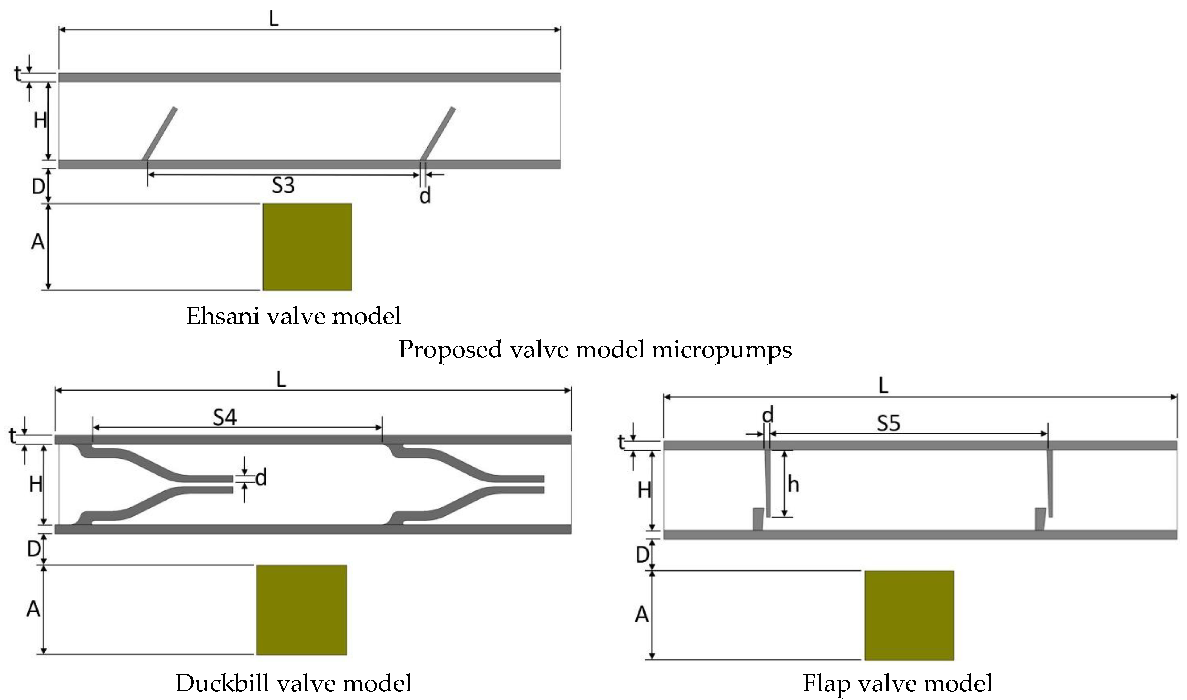
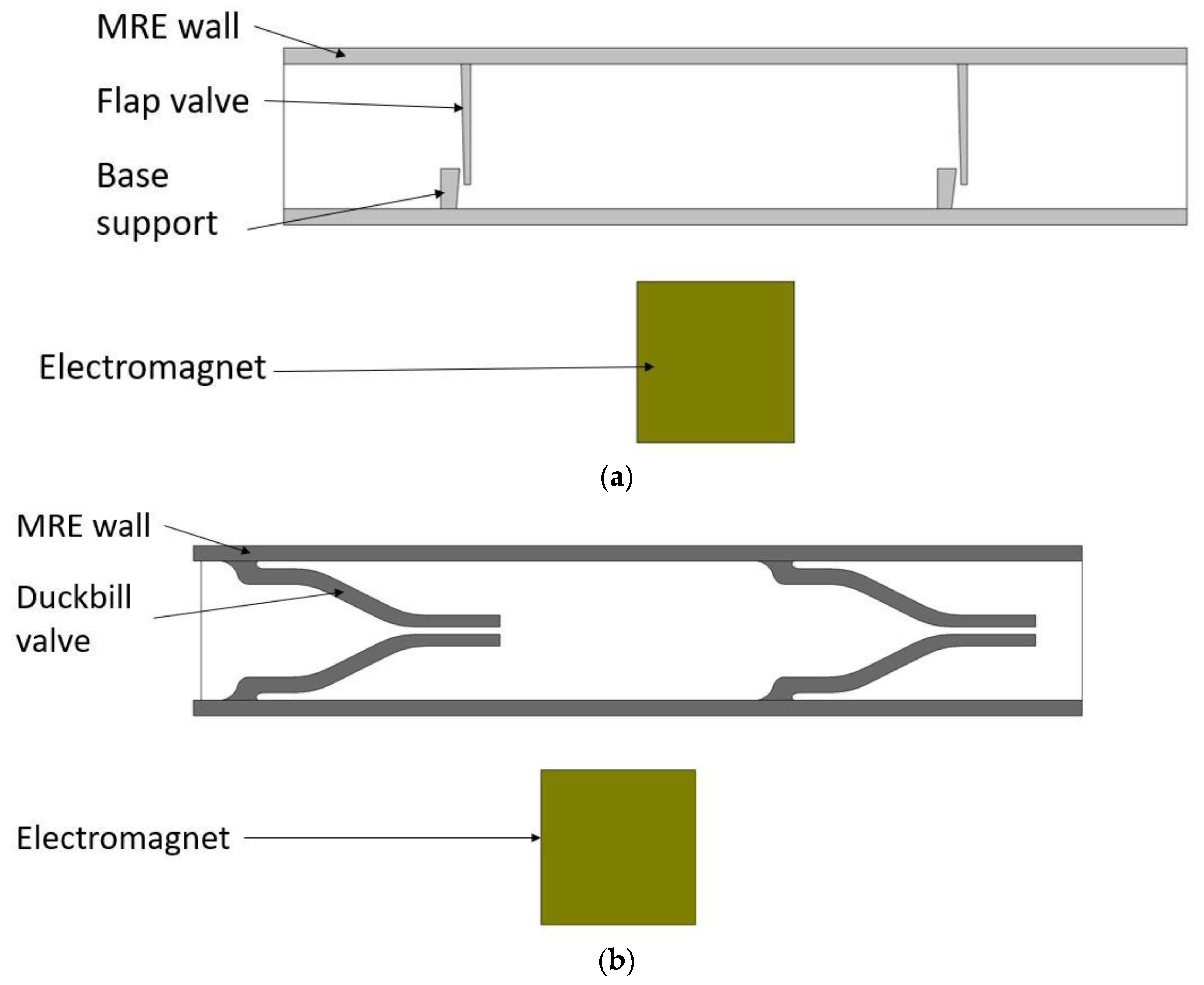
2. Proposed Design
3. Simulation Methodology
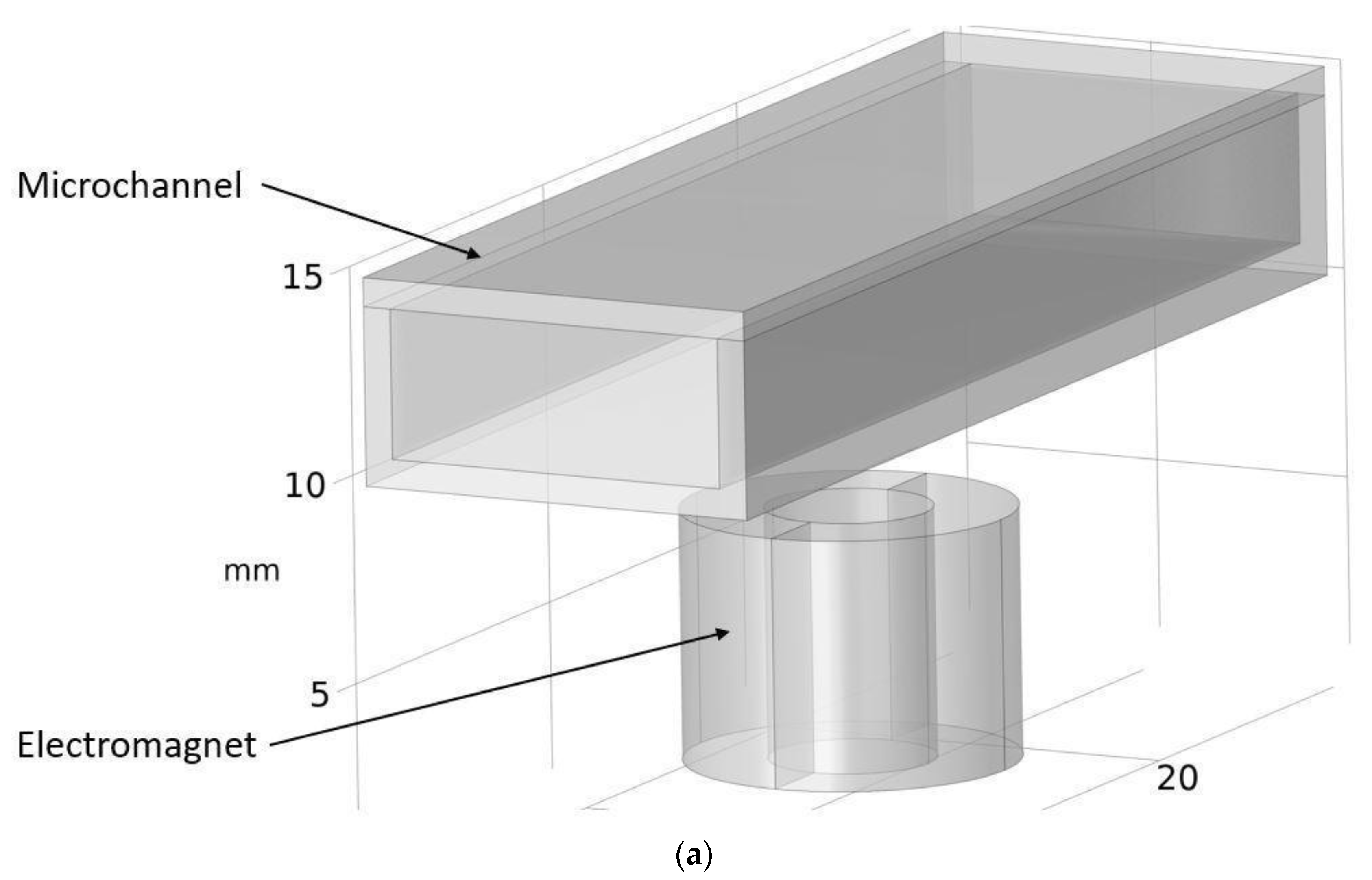
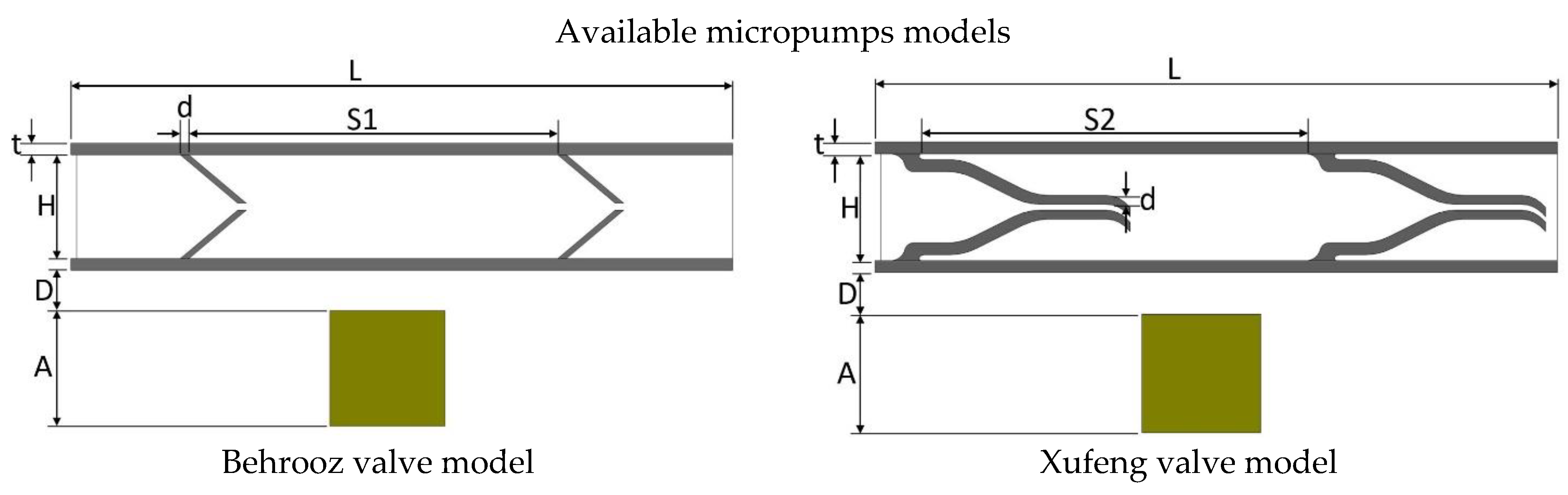
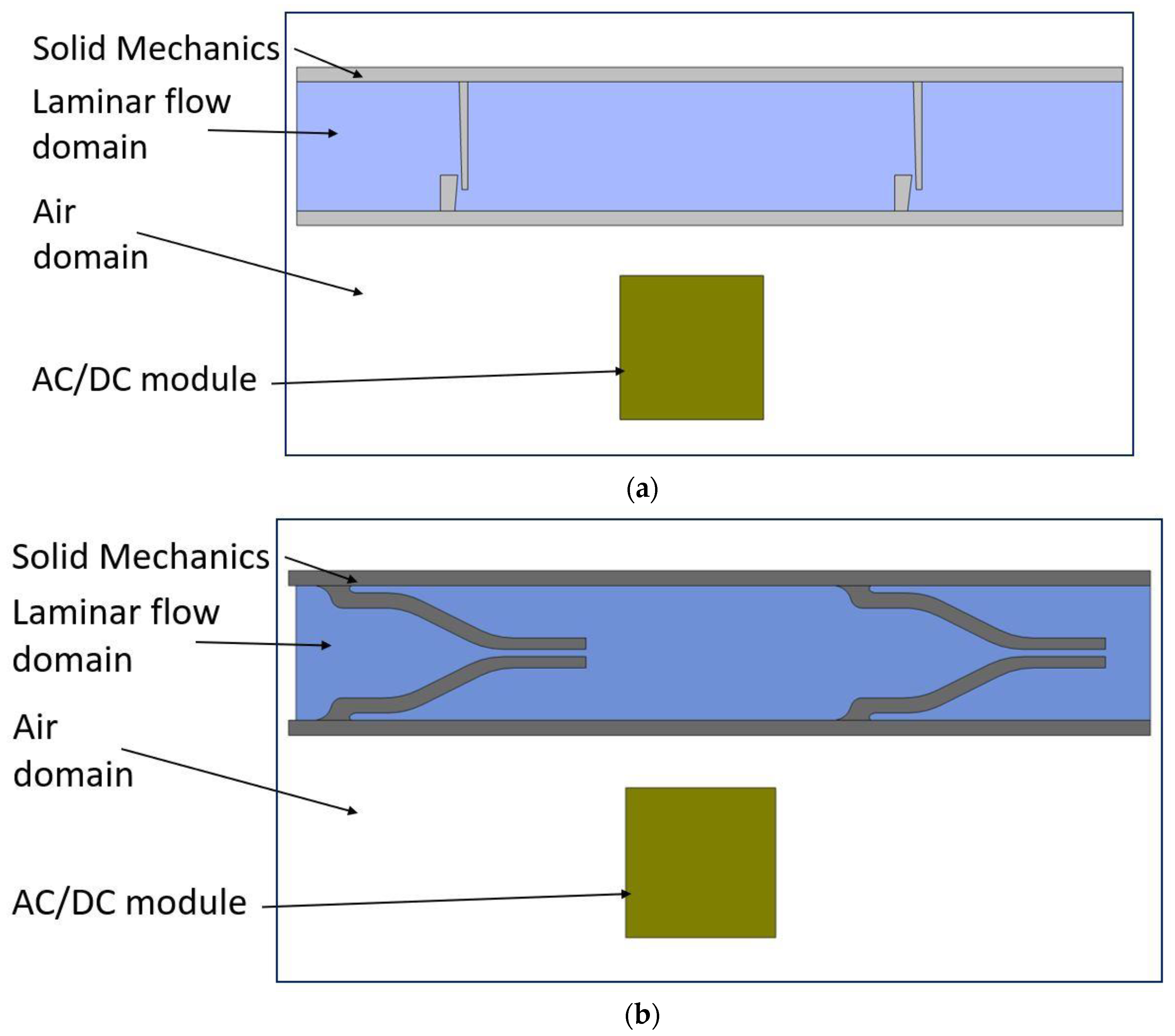
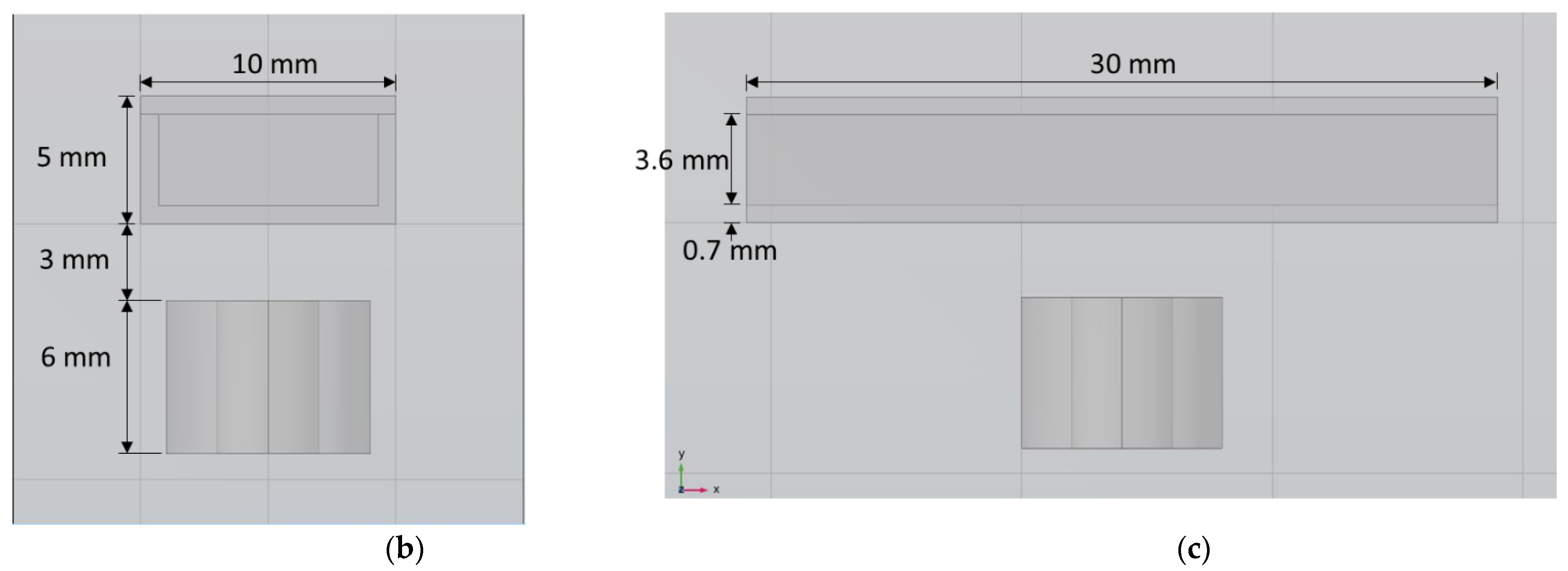
3.1. Model Creation
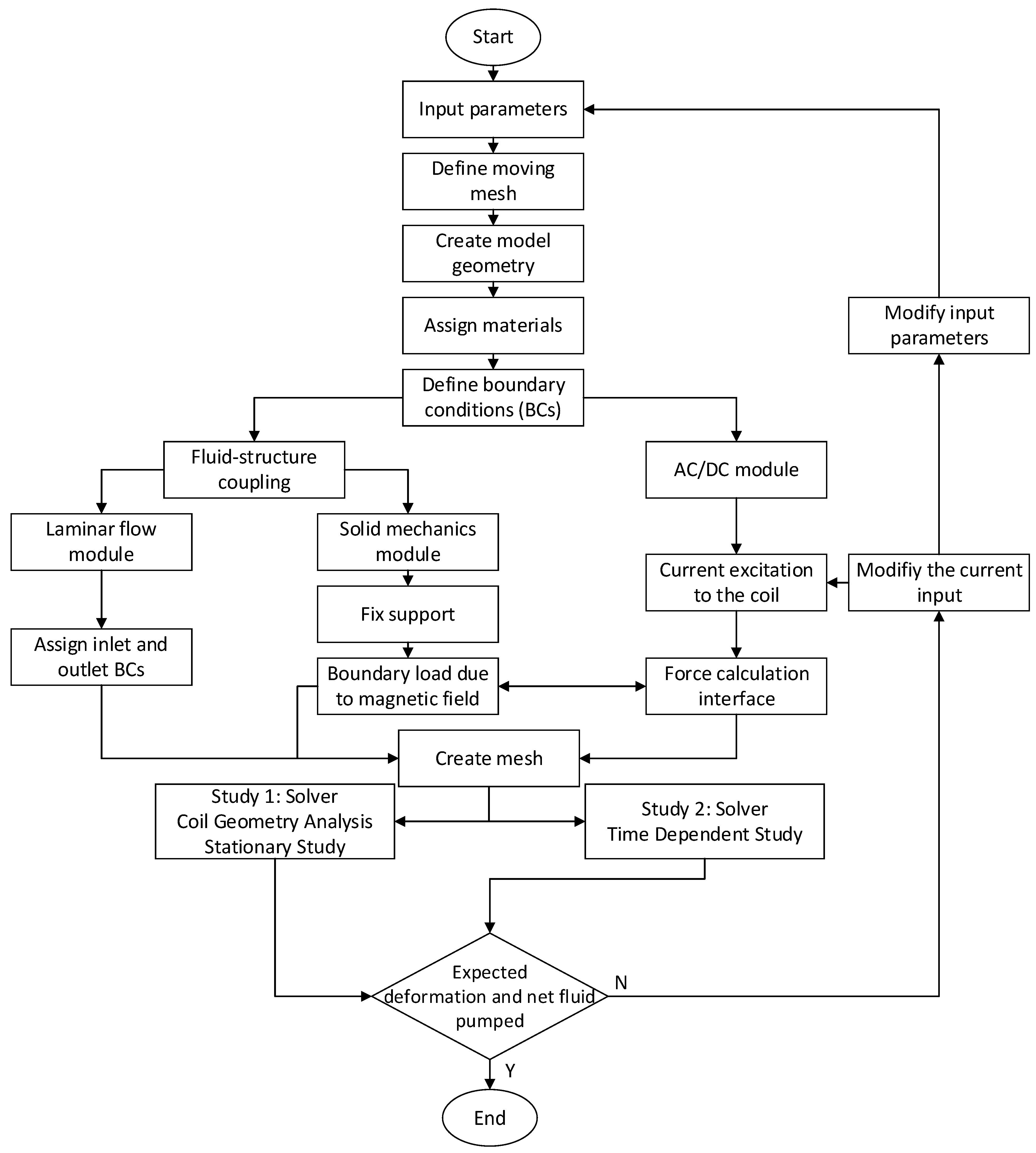
3.2. Simulation Procedure
3.3. Boundary Conditions
3.4. Computing Equations
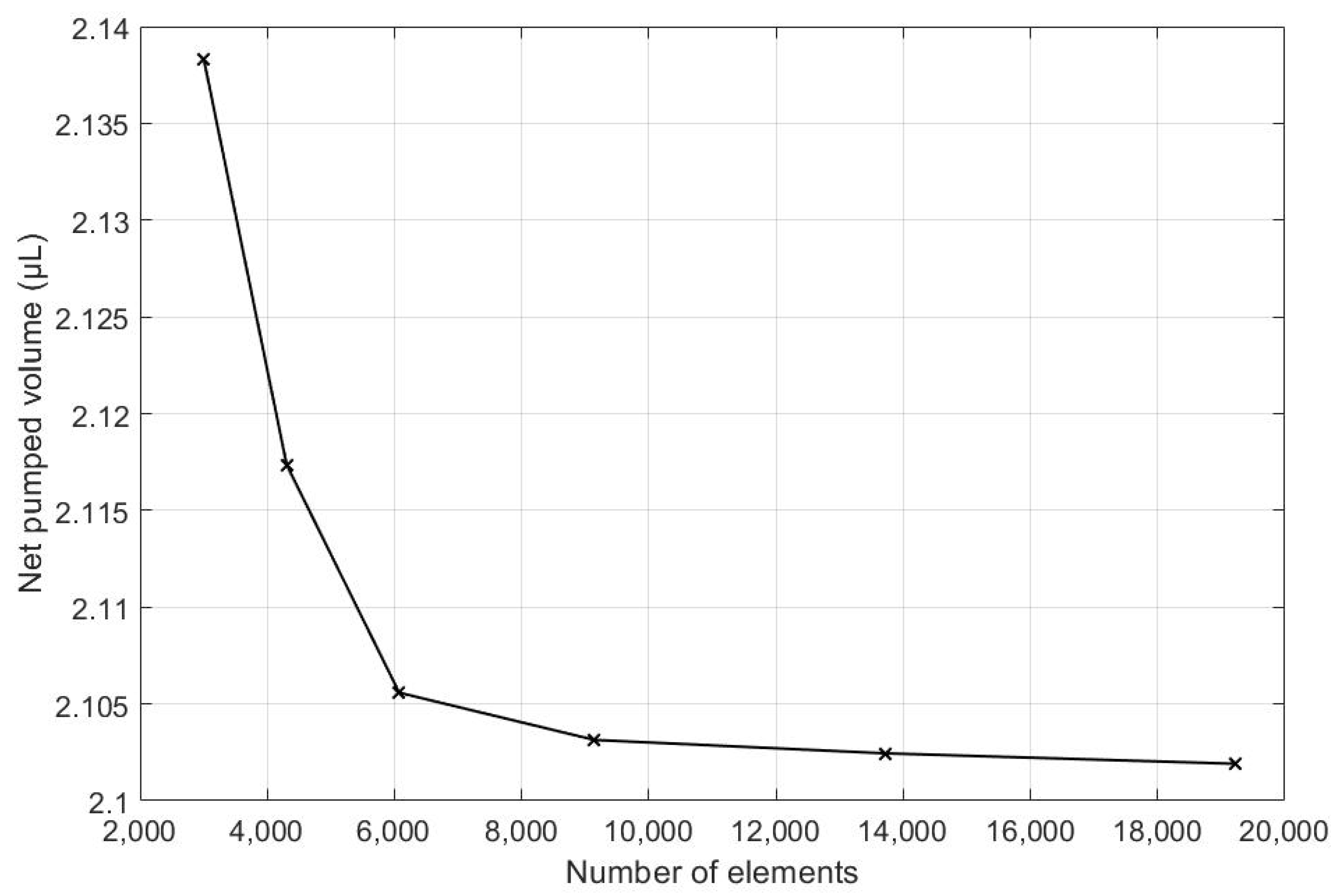
3.5. Grid Generation and Grid Independence Study
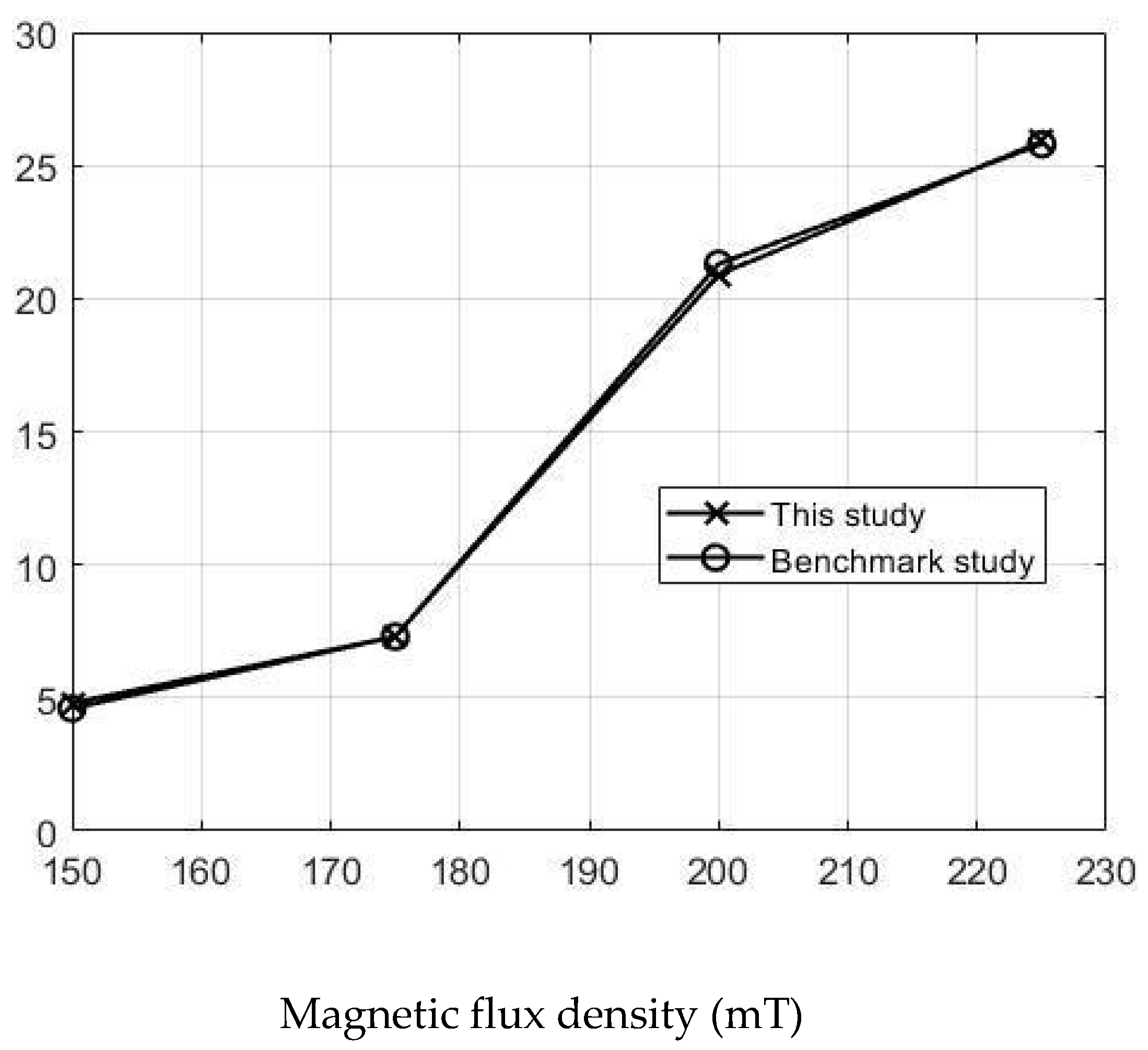
3.6. Validity Study
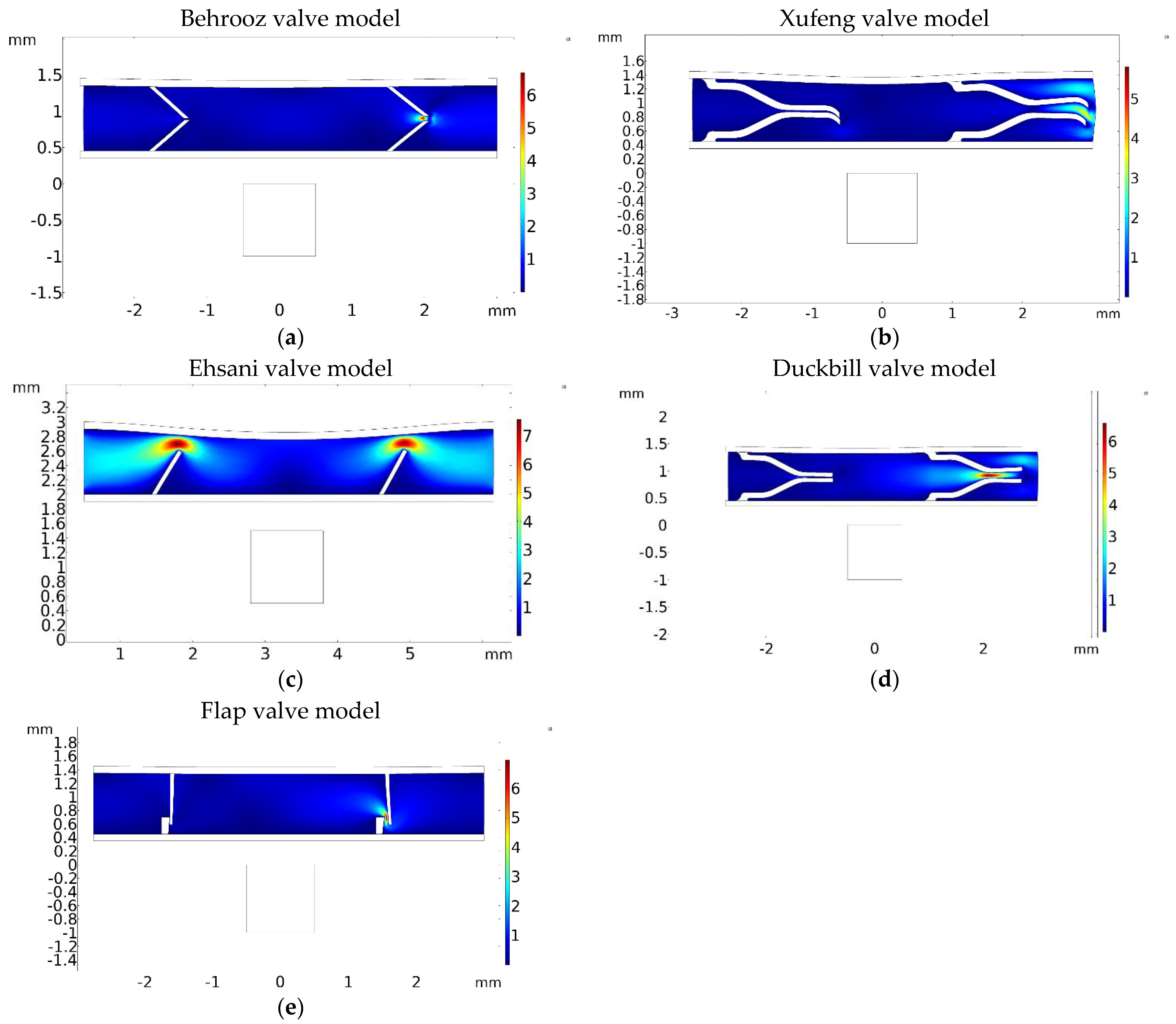
3.7. Results and Discussions
4. Summary and Conclusions
- The comparison study revealed that:
- ○
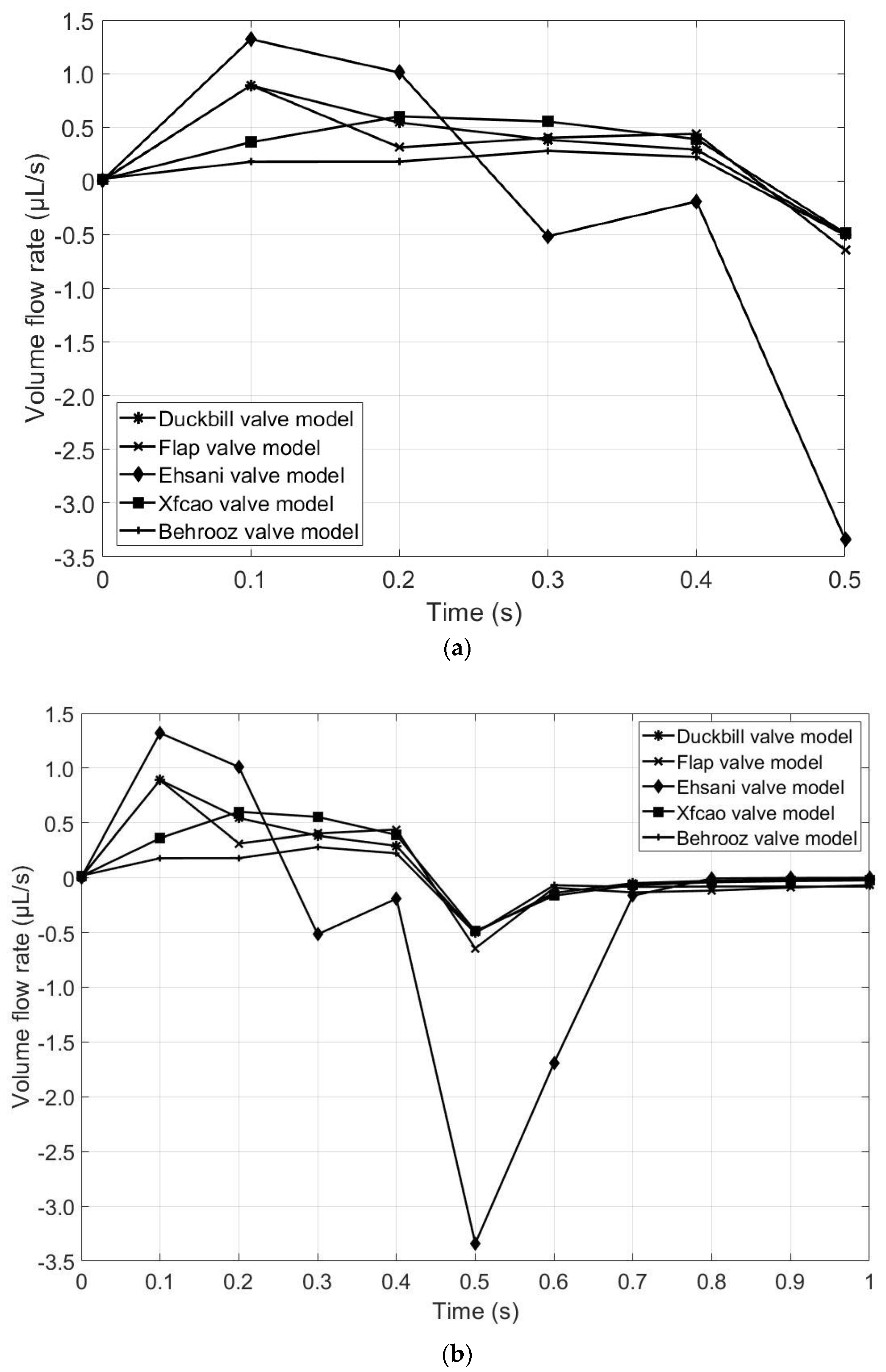
- the proposed duckbill and flap valve micropumps were five times faster than the Ehsani and Xufeng valve micropumps;
- ○
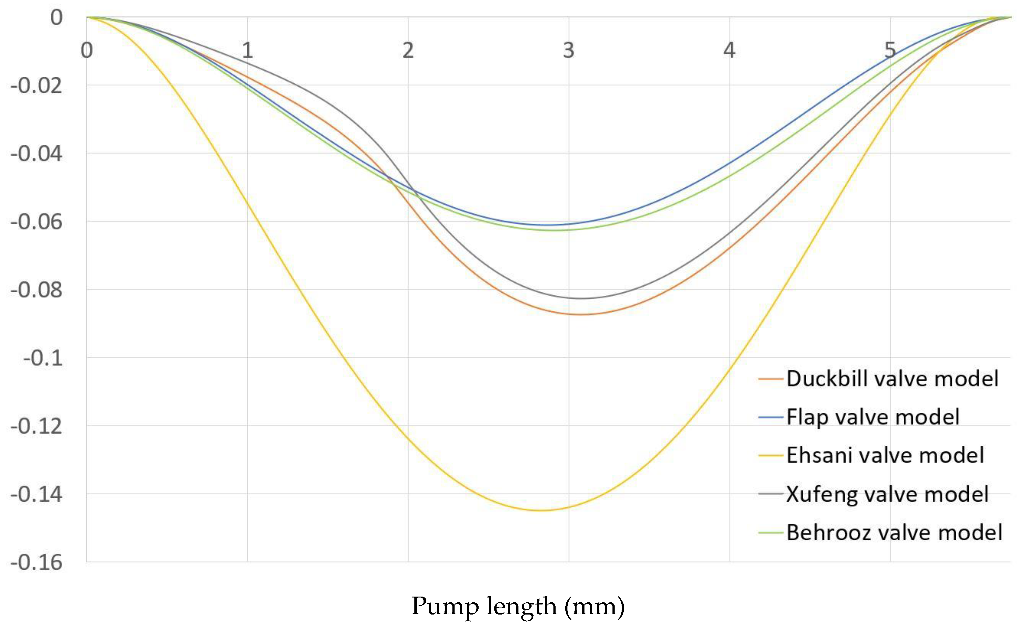
- the backflow was comparatively less for the duckbill and flap valve micropumps, while the Ehsani models showed the maximum backflow;
- ○
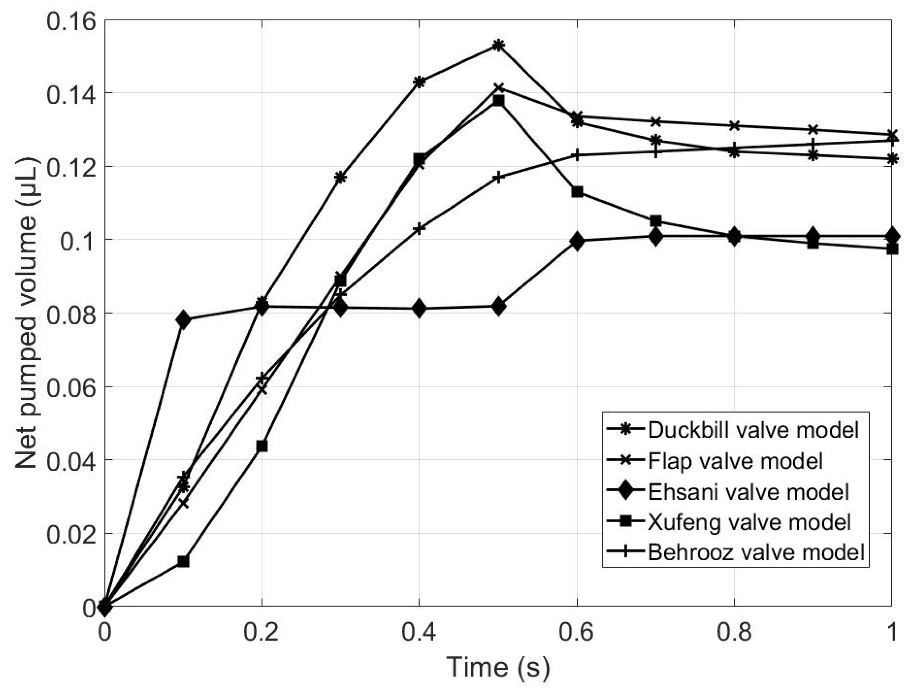
- the proposed flap and duckbill valve model could pump 1.09 µL and 1.16 µL in 1 s of pumping cycle, respectively, which is more than each of the three existing micropump models.
- After examining the MRE wall deformation, velocity magnitude and volume flow rate, it is concluded that the proposed duckbill and flap valve models can propel the largest amount fluid in the same time interval, and both of them have short response time to apply the magnetic field. Thus, in terms of the performance measures, it can be concluded that the proposed two models provide better results.
- The proposed study could be used for future MR micropump design considerations.
Author Contributions
Funding
Institutional Review Board Statement
Informed Consent Statement
Data Availability Statement
Acknowledgments
Conflicts of Interest
References
- Behrooz, F.; Wang, M.; Gordaninejad, X. Seismic Control of Base Isolated Structures Using Novel Magnetorheological Elastomeric Bearing. In Proceedings of the SMASIS2013, Snowbird, UT, USA, 16–18 September 2013; pp. 1–9. [Google Scholar] [CrossRef]
- Yarra, S.; Behrooz, M.; Pekcan, G.; Itani, A.; Gordaninejad, F. A large-scale adaptive magnetorheological elastomer-based bridge bearing. In Proceedings of the Active and Passive Smart Structures and Integrated Systems 2017, Portland, OR, USA, 11 April 2017; Volume 10164, p. 1016425. [Google Scholar] [CrossRef]
- Behrooz, M.; Yarra, S.; Mar, D.; Pinuelas, N.; Muzinich, B.; Publicover, N.G.; Pekcan, G.; Itani, A.; Gordaninejad, F. A self-sensing magnetorheological elastomer-based adaptive bridge bearing with a wireless data monitoring system. In Proceedings of the Sensors and Smart Structures Technologies for Civil, Mechanical, and Aerospace Systems 2016, Las Vegas, NV, USA, 26 July 2016; Volume 9803, p. 98030D. [Google Scholar] [CrossRef]
- Syam, T.M.I.; Muthalif, A.G.A. Magnetorheological Elastomer based torsional vibration isolator for application in a prototype drilling shaft. J. Low Freq. Noise Vib. Act. Control 2021, 41, 1–25. [Google Scholar] [CrossRef]
- An, H.N.; Sun, B.; Picken, S.J.; Mendes, E. Long time response of soft magnetorheological gels. J. Phys. Chem. B 2012, 116, 4702–4711. [Google Scholar] [CrossRef] [PubMed]
- Carlson, J.D.; Jolly, M. MR fluid, foam and elastomer devices. Mechatronics 2000, 10, 555–569. [Google Scholar] [CrossRef]
- Davis, L.C. Model of magnetorheological elastomers. J. Appl. Phys. 1999, 85, 3348–3351. [Google Scholar] [CrossRef]
- Ginder, J.M.; Davis, L.C. Shear stresses in magnetorheological fluids: Role of magnetic saturation. Appl. Phys. Lett. 1994, 65, 3410–3412. [Google Scholar] [CrossRef]
- Gong, X.; Xu, Y.; Xuan, S.; Guo, C.; Zong, L. The investigation on the nonlinearity of plasticine-like magnetorheological material under oscillatory shear rheometry. J. Rheol. 2012, 56, 1375–1391. [Google Scholar] [CrossRef] [Green Version]
- Oliveira, F.; Botto, M.A.; Morais, P.; Suleman, A. Semi-active structural vibration control of base-isolated buildings using magnetorheological dampers. J. Low Freq. Noise Vib. Act. Control 2018, 37, 565–576. [Google Scholar] [CrossRef]
- Rabinow, J. The magnetic fluid clutch. Electr. Eng. 1948, 67, 1167. [Google Scholar] [CrossRef]
- Rodríguez-López, J.; Elvira, L.; Resa, P.; Montero De Espinosa, F. Sound attenuation in magnetorheological fluids. J. Phys. D Appl. Phys. 2013, 46, 065001. [Google Scholar] [CrossRef]
- Song, W.L.; Li, D.H.; Tao, Y.; Wang, N.; Xiu, S.C. Simulation and experimentation of a magnetorheological brake with adjustable gap. J. Intell. Mater. Syst. Struct. 2017, 28, 1614–1626. [Google Scholar] [CrossRef]
- Sun, S.; Peng, X.; Guo, Z. Study on macroscopic and microscopic mechanical behavior of magnetorheological elastomers by representative volume element approach. Adv. Condens. Matter Phys. 2014, 2014, 232510. [Google Scholar] [CrossRef] [Green Version]
- Behrooz, M.; Gordaninejad, F. A flexible micro fluid transport system featuring magnetorheological elastomer. Smart Mater. Struct. 2016, 25, 025011. [Google Scholar] [CrossRef]
- Behrooz, M.; Gordaninejad, F. Three-dimensional study of a one-way, flexible magnetorheological elastomer-based micro fluid transport system. Smart Mater. Struct. 2016, 25, 095012. [Google Scholar] [CrossRef]
- Ehsani, A.; Nejat, A. Conceptual design and performance analysis of a novel flexible-valve micropump using magneto-fluid-solid interaction. Smart Mater. Struct. 2017, 26, 055036. [Google Scholar] [CrossRef]
- Cao, X.; Xuan, S.; Hu, T.; Gong, X. 3D printing-assistant method for magneto-active pulse pump: Experiment, simulation, and deformation theory. Appl. Phys. Lett. 2020, 117, 241901. [Google Scholar] [CrossRef]


| Micropump Models | Number of Electromagnets | Valve Type | Upper Wall Material | Parametric Study | Simulation |
|---|---|---|---|---|---|
| Behrooz valve model | 1 | One-way conical valve | MRE | Yes | MFSI |
| Xufneg valve model | 1 | Check valve | MRE | No | No |
| Ehsani valve model | 1 | One-way angle valve | MRE | Yes | MFSI |
| Parameter | Symbol | Behrooz Valve Model | Xufeng Valve Model | Ehsani Valve Model | Duckbill Valve Model | Flap Valve Model |
|---|---|---|---|---|---|---|
| Height of the pump chamber | H | 0.9 (mm) | 0.9 (mm) | 0.9 (mm) | 0.9 (mm) | 0.9 (mm) |
| Thickness of the upper wall | t | 0.1 (mm) | 0.1 (mm) | 0.1 (mm) | 0.1 (mm) | 0.1 (mm) |
| Valve spacing distance | S | S1 = 3.079 (mm) | S2 = 3.238 (mm) | S3 = 3.069 (mm) | S4 = 3.204 (mm) | S5 = 3.102 (mm) |
| Length of micro channel | L | 5.65 (mm) | 5.65 (mm) | 5.65 (mm) | 5.65 (mm) | 5.65 (mm) |
| Distance between the pump chamber and electromagnet | D | 0.35 (mm) | 0.35 (mm) | 0.35 (mm) | 0.35 (mm) | 0.35 (mm) |
| Side of the electromagnet | A | 1 (mm) | 1 (mm) | 1 (mm) | 1 (mm) | 1 (mm) |
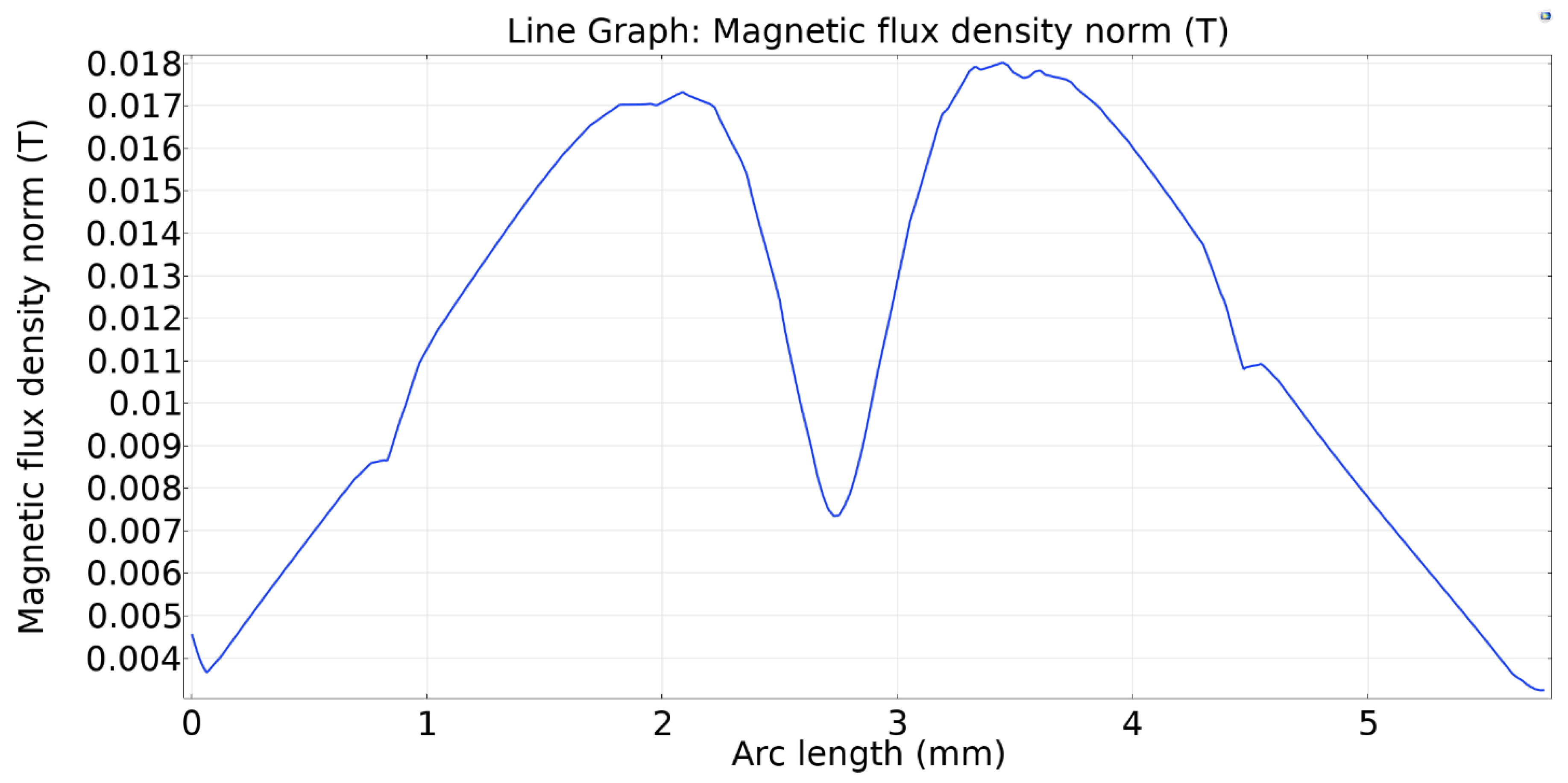
| Magnetic flux density | B | 0.018 (T) | 0.018 (T) | 0.018 (T) | 0.018 (T) | 0.018 (T) |
| Elastic modulus | E | 1.2 (MPa) | 1.2 (MPa) | 1.2 (MPa) | 1.2 (MPa) | 1.2 (MPa) |
| Grid Number | Number of Mesh Elements | Net Pumped Volume (µL) | The Difference in Net Pumped Volume (%) |
|---|---|---|---|
| 1 | 3002 | 2.13832 | - |
| 2 | 4306 | 2.11735 | 0.98 |
| 3 | 6075 | 2.10558 | 0.56 |
| 4 | 9144 | 2.10314 | 0.51 |
| 5 | 13,708 | 2.10245 | 0.14 |
| 6 | 19,215 | 2.10191 | 0.11 |
| Magnetic Flux Density (mT) | Benchmark Study ”Reprinted/Adapted with Permission from Ref. [18]. 2022, Rubayet Hassan”. | This Study | Maximum Displacement of Upper Wall (mm) |
|---|---|---|---|
| 75 | 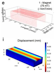 |  | 0.4 |
| 145 |  |  | 1.2 |
| 175 |  |  | 3.4 |
| Magnetic Flux Density (mT) | Magnetic Flux Density (mT) | Flow Rate from Validation Case (µL/s) | Percentage of Error (%) |
|---|---|---|---|
| 150 | 4.8 | 4.6 | 4.16 |
| 175 | 7.3 | 7.3 | 0 |
| 200 | 20.9 | 21.3 | 1.91 |
| 225 | 25.9 | 25.8 | 0.39 |
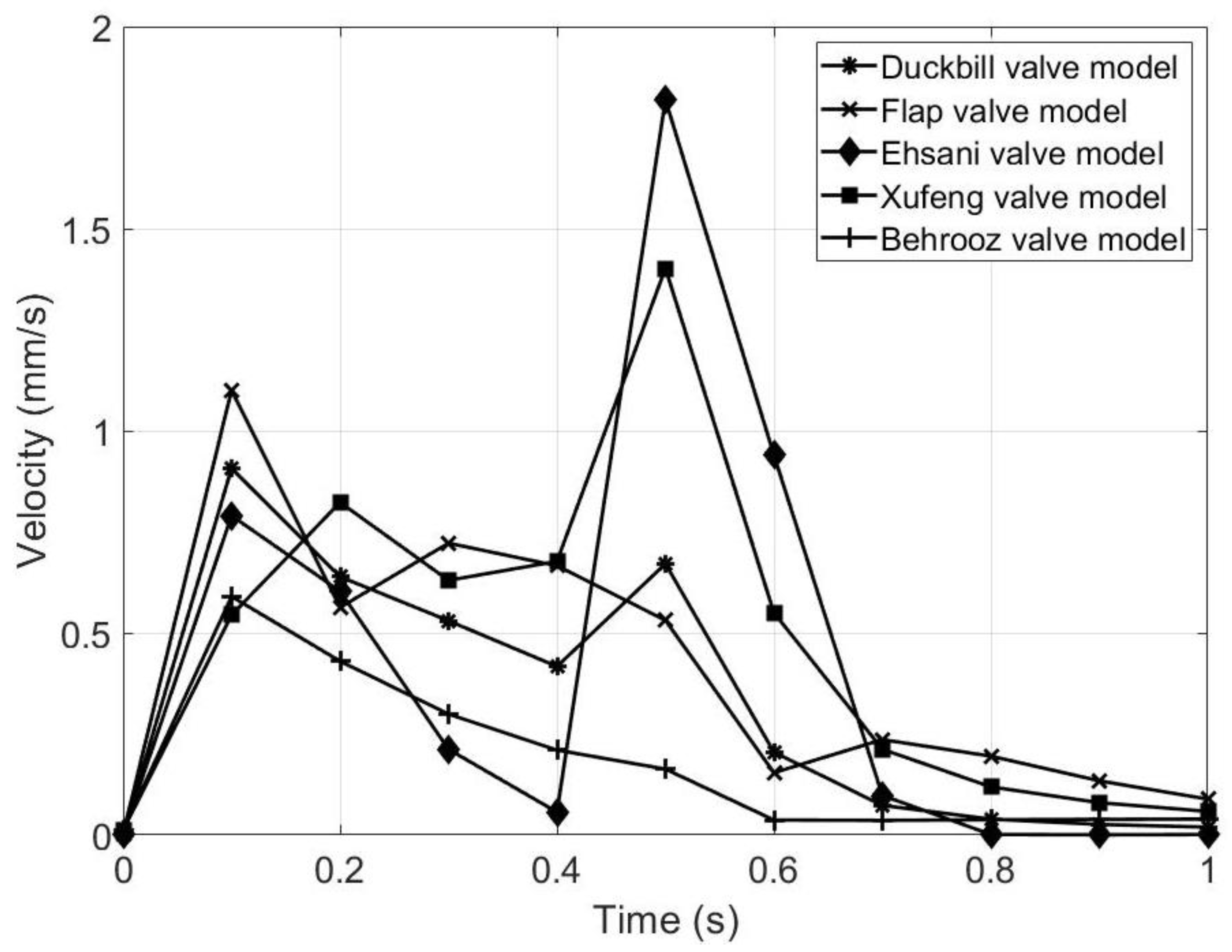
| Valve Model | Maximum Velocity Occurred (s) | Maximum Velocity Magnitude at Outlet (mm/s) |
|---|---|---|
| Flap valve | 0.1 | 1.10 |
| Duckbill valve | 0.1 | 0.91 |
| Behrooz valve | 0.1 | 0.59 |
| Ehsani Valve | 0.5 | 1.82 |
| Xufeng valve | 0.5 | 1.40 |
| Micropump Model | Net Pumped Volume (µL) |
|---|---|
| Duckbill valve model | 1.16 |
| Flap valve model | 1.09 |
| Xufeng valve model | 0.92 |
| Ehsani valve model | 0.91 |
| Behrooz valve model | 1.03 |
Publisher’s Note: MDPI stays neutral with regard to jurisdictional claims in published maps and institutional affiliations. |
© 2022 by the authors. Licensee MDPI, Basel, Switzerland. This article is an open access article distributed under the terms and conditions of the Creative Commons Attribution (CC BY) license (https://creativecommons.org/licenses/by/4.0/).
Share and Cite
Cesmeci, S.; Hassan, R.; Baniasadi, M. A Comparative Evaluation of Magnetorheological Micropump Designs. Micromachines 2022, 13, 764. https://doi.org/10.3390/mi13050764
Cesmeci S, Hassan R, Baniasadi M. A Comparative Evaluation of Magnetorheological Micropump Designs. Micromachines. 2022; 13(5):764. https://doi.org/10.3390/mi13050764
Chicago/Turabian StyleCesmeci, Sevki, Rubayet Hassan, and Mahmoud Baniasadi. 2022. "A Comparative Evaluation of Magnetorheological Micropump Designs" Micromachines 13, no. 5: 764. https://doi.org/10.3390/mi13050764
APA StyleCesmeci, S., Hassan, R., & Baniasadi, M. (2022). A Comparative Evaluation of Magnetorheological Micropump Designs. Micromachines, 13(5), 764. https://doi.org/10.3390/mi13050764