1. Introduction
Laser processing has the characteristics of high speed and stable energy. These properties have led to the widespread adoption of laser processing in the manufacturing, automotive, and electronics industries. Lasers can be applied in various ways, including cutting specific shapes on diamonds [
1], material removal on CBN (cubic boron nitride) [
2], drilling YSZ (yttrium stabilized zirconia) materials [
3], micro-drilling aluminum materials [
4], drilling holes without creating cracks on surfaces [
5], and sintering materials [
6]. However, controlling the depth of blind holes in laser drilling remains a challenge. In fact, the depth of laser-drilled holes is affected by many factors, such as the energy of the laser pulse, the pulse frequency, properties of the material being worked, spatter, and gas pressure. Controlling high-aspect-ratio blind holes with small diameters represents even more of a challenge, as accurately controlling the depth of blind holes in laser drilling requires a substantial amount of effort [
7]. Daniel et al. [
8] presented a mathematical model to estimate the drilled hole depth based on the homogenous distribution radiation of the laser on the wall of the drilled holes. However, it must be assumed that the drilled hole is conical, and it might not be suitable in cases full of variables. Numerical simulation techniques have also been applied to predict the depth and processing time in the laser drilling process. Meshless and particle-based methods were suitable for the simulation of the laser ablation process regarding its material loss in the process. The smoothed particle hydrodynamics (SPH) modeling technique was used to model the transient heat conduction during the interaction between the laser and material [
9]. In order to improve the robustness and efficiency of the computational calculation, several techniques have been developed, such as the particle strength exchange (PSE) method [
10], the symmetric smoothed-particle hydrodynamics (SSPH) method [
11], or the meshless local Petrov–Galerkin (MLPG) collocation method [
12]. A three-dimensional simulation of the laser drilling process by meshless methods with six different schemes was performed to compare runtimes at three different resolutions of particles [
13]. With numerical simulation techniques, however, process variables, for example, absorptivity of material, latent heat, or assist gas, were ignored in the computational modeling.
Neural networks can construct nonlinear models, can accept different kinds of variables as input, and have strong adaptability. They have been used for prediction, modeling, and parameter optimization in various laser processing techniques in recent years. One study indicated that artificial intelligence could extract knowledge concealed in experimental data, so that complex decisions could be made without manual intervention [
14]. In 2003, Yousef employed a neural network to predict laser energy using just the material type, drilling depth, and diameter for single-shot laser processing as inputs. This investigation demonstrated that neural networks can be used to predict the required processing parameters [
15].
Since artificial neural networks (ANNs) can only determine parameter conditions through constant recalculation, they may not provide the best processing solution. For this reason, Solati et al. [
16] combined an ANN with a genetic algorithm (GA), using the ANN to process the relationship equation first for material removal, and then using the GA to optimize the parameters. Sibalija et al. [
17] proposed a method of integrating ANNs with GA and compared this design with Taguchi’s quality loss function. Experimental laser drilling results showed that the integration of an ANN generated a system that could find a global solution within a continuous space.
In addition to optimizing ANNs, a GA can also be used alone to generate predictive algorithms. In one study, a GA was employed to establish multi-gene genetic programming (MGGP). Subsequently, scholars compared outcomes between ANNs when combined with MGGP, predicting the strength and processing time of processed graphene sheets using processing temperature, drill speed, and drill feed. Their results showed that MGGP-enhanced ANNs significantly outperformed conventional ANNs [
18].
Patel et al. [
19] compared the accuracy of fuzzy logic, regression models, and ANNs when predicting groove widths in laser-cut, glass-fiber-reinforced polymers. As input parameters, they tested changes in laser power, auxiliary gas pressure, and cutting speed. Mustafa et al. [
20] compared the results of extreme learning machines (ELMs) with ANNs to predict droplet spatter area, hole diameter, and hole inclination for the laser drilling of a titanium alloy, a material commonly used in aerospace engineering. In this study, not only was the ELM model more accurate than the ANN, but its operation time was shorter.
Another study incorporated analysis of variance into the response surface methodology (RSM) to enhance prediction accuracy, and then compared it with a feed-forward, back-propagation ANN to predict groove depth, groove width, and pattern similarity for machined Al–SiC composites. The input parameters comprised auxiliary gas flow, focus position, pulse frequency, and laser current. Overall, the ANN demonstrated a more uniform performance [
21]. Dhaker et al. [
22] used an adaptive neuro-fuzzy inference system that combined a GA and fuzzy logic to optimize parameters. It achieved accurate results by governing control parameters.
Most of the study works focused on predicting process parameters or predicting drilling depth and geometry, separately. Thus, this study proposes a complete architecture combining process parameter prediction and processing result simulation. With the proposed method, the operator only needs to input the desired drilling depth and hole diameter, and then the system can predict the required process parameters. At the same time, the proposed system can also simulate the processing results, and the operator can check whether the simulation error is within the acceptable range as the basis for whether to adjust the parameters. Through such a pre-simulation, the number of trial parameters can be reduced and the preparation time of finding parameters can be shortened. The quality of the drilled holes can also be confirmed in advance.
2. Pre-Processing of the Experiment
The laser source in this study was a 20-W EP-Z Pulsed Fiber Laser (PFL). Detailed specifications of the experimental setup are presented in
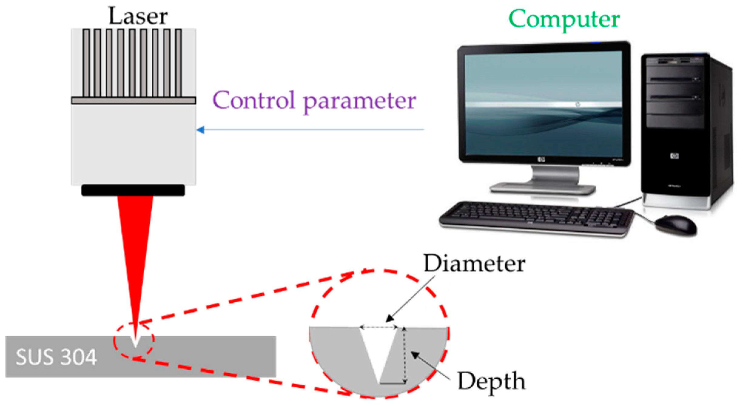
Table 1. A schematic figure of laser drilling is shown in
Figure 1. The processing material selected for testing was 304 stainless steel, 50 mm × 50 mm × 2 mm with a surface roughness Ra of 0.07.
Table 2 shows the precise material composition provided by the stainless steel manufacturer.
Before processing, an ultrasonic vibration machine was used to clean the surface of the material with acetone and ethanol for 20 and 25 s, respectively. The focus position was located on the surface of the material. Each hole’s drilling location was located 0.5 mm apart. To ensure experimental reliability and reproducibility, the position of the material and the z-axis of the laser processing machine were not adjusted when the material was placed onto the laser machining platform.
2.1. Experimental Data Collection
Many factors affect laser processing results, including laser pulse width, pulse repetition frequency, pulse waveform, pulse energy, number of pulses, and auxiliary gas pressure. The amount of laser energy applied to the material surface directly affects the laser drilling depth; therefore, among these factors, the combination of laser pulse energy and number of pulses is the most direct factor affecting drilling depth. Therefore, this study selected these two factors as the key variables of interest and held other parameters fixed for the duration of the experiment. The laser pulse energy settings used in this study were 0.45, 0.475, and 0.5 mJ. The number of shots used ranged from 1 to 40. Each combination of shots at each energy level were performed nine times for reliability, thus obtaining 1080 sets of data. Each data set contained the laser pulse energy, number of shots, drilled-hole diameter, and depth.
2.2. Measurement of Hole Diameter and Depth
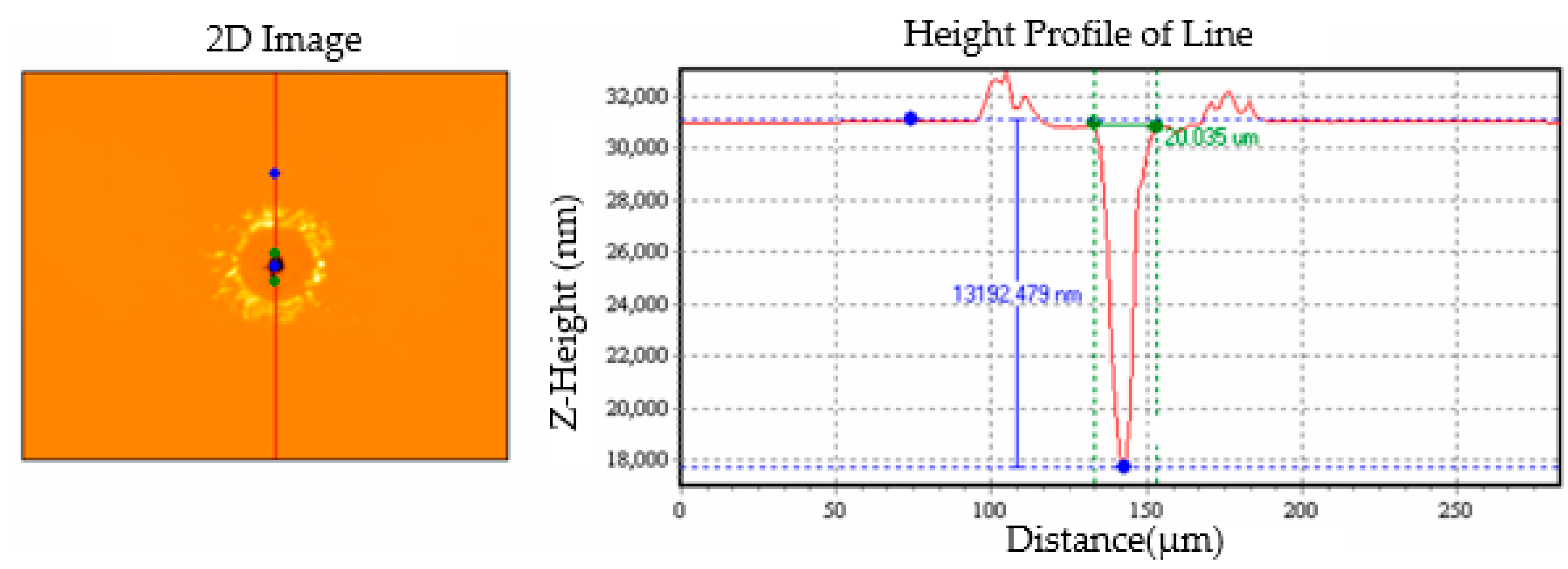
In order to reduce any errors caused by measurement and to ensure that the measurements were as accurate as possible, we used two types of instruments to measure the diameter and depth of the drilled holes. The first instrument was a SWIM-1510MS white-light interferometer obtained from Taizhi Precision Technology Company. It has a measurement accuracy of 1 nm increments and was used to measure the depth of shallow drilled holes. The measurement method is illustrated in
Figure 2.
Where the number of shots exceeded 10, the drilled-hole depth could not be measured accurately with a white-light interferometer. Therefore, a microscopy with an Olympus U-PMVTC was used in focus mode with a resolution of 0.5 μm. By using this instrument, the hole diameters were also measured from the captured images, as shown in
Figure 3.
3. Methodology
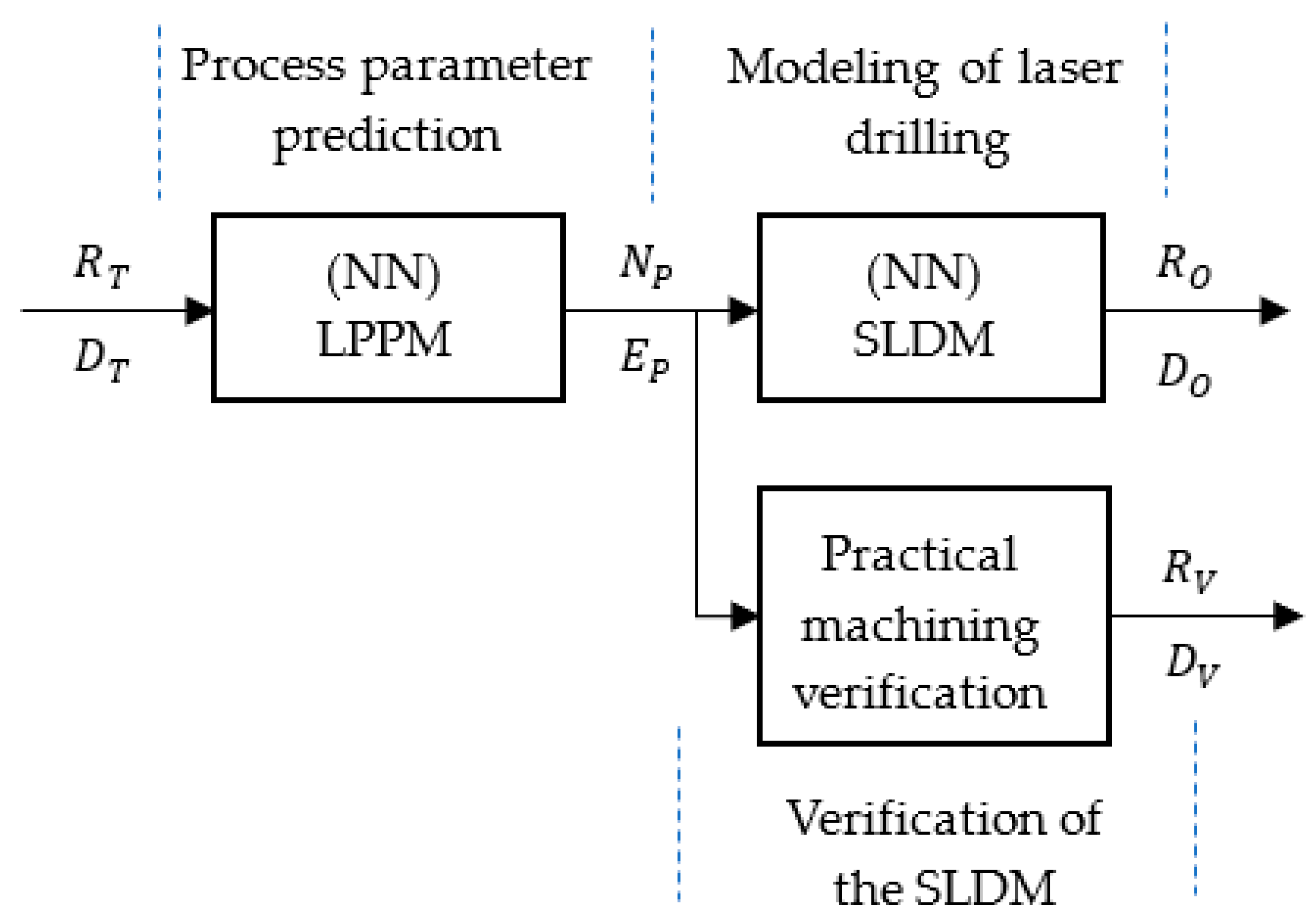
This study established two neural network models based on the deep learning toolbox in MATLAB and combined these with the practical laser machining process shown in
Figure 4. First, the target diameter
RT and target depth
DT data were fed into the laser parameter prediction model (LPPM). The number of laser shots
NP and the laser pulse energy
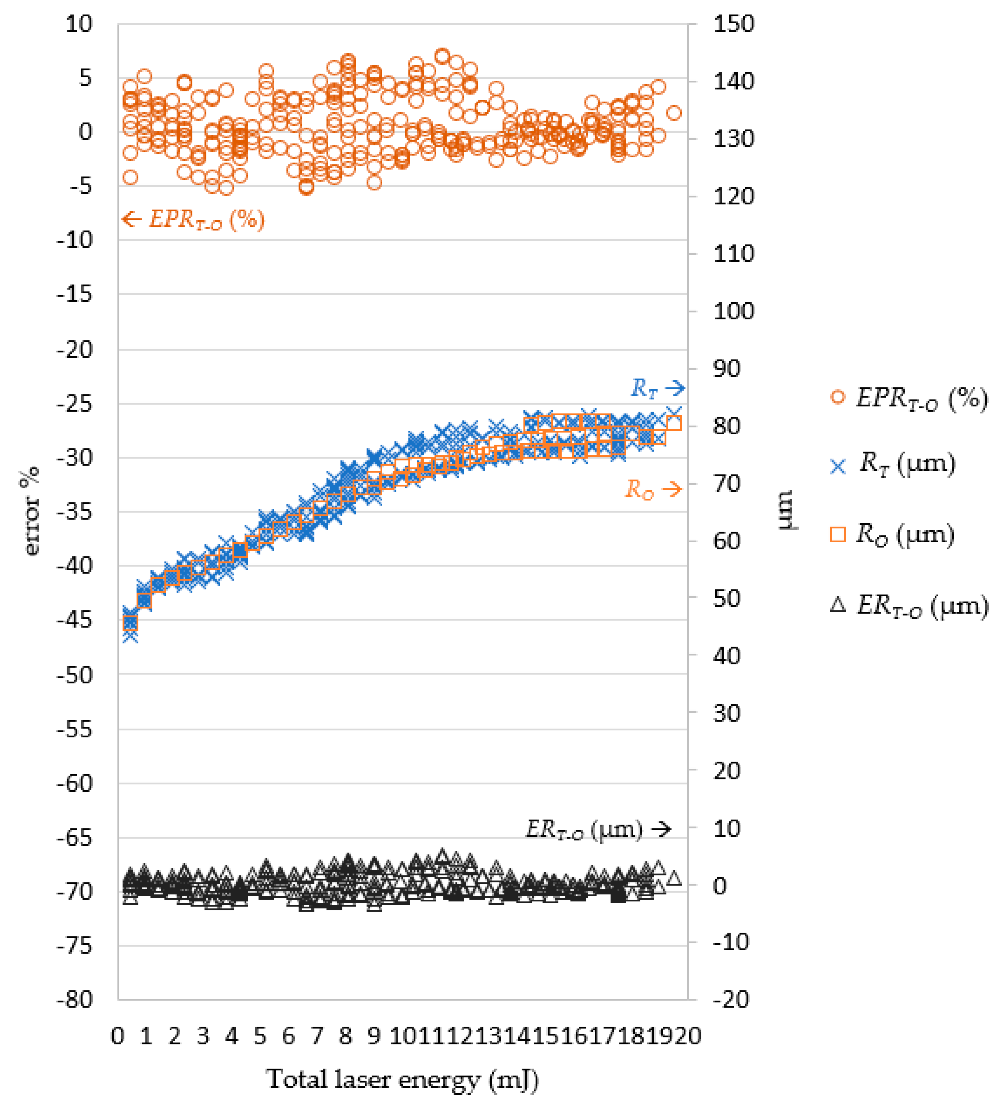
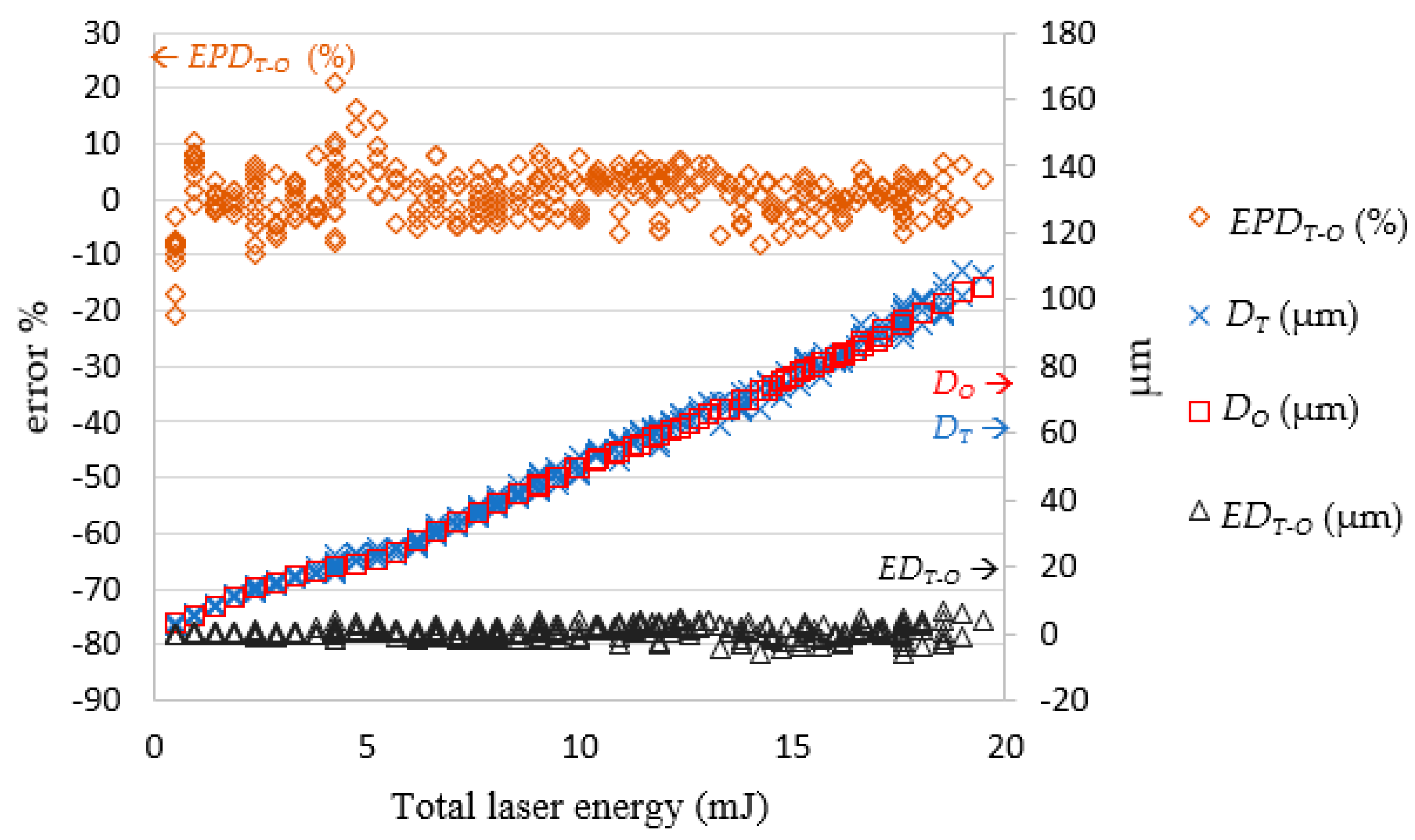
EP required were given in the output. Second, the LPPM output was then input to the simulated laser drilling model (SLDM) to simulate the drilling results and provide the values of the simulated hole diameter
RO and depth
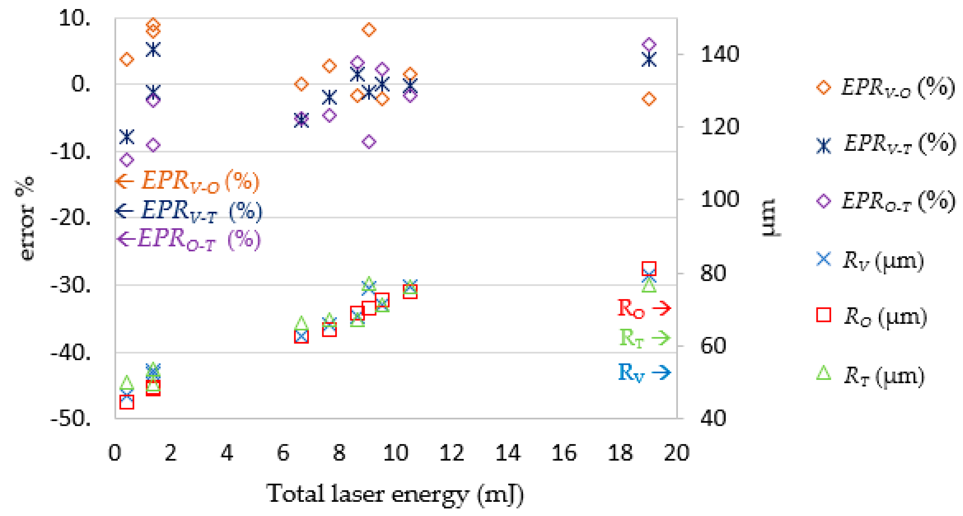
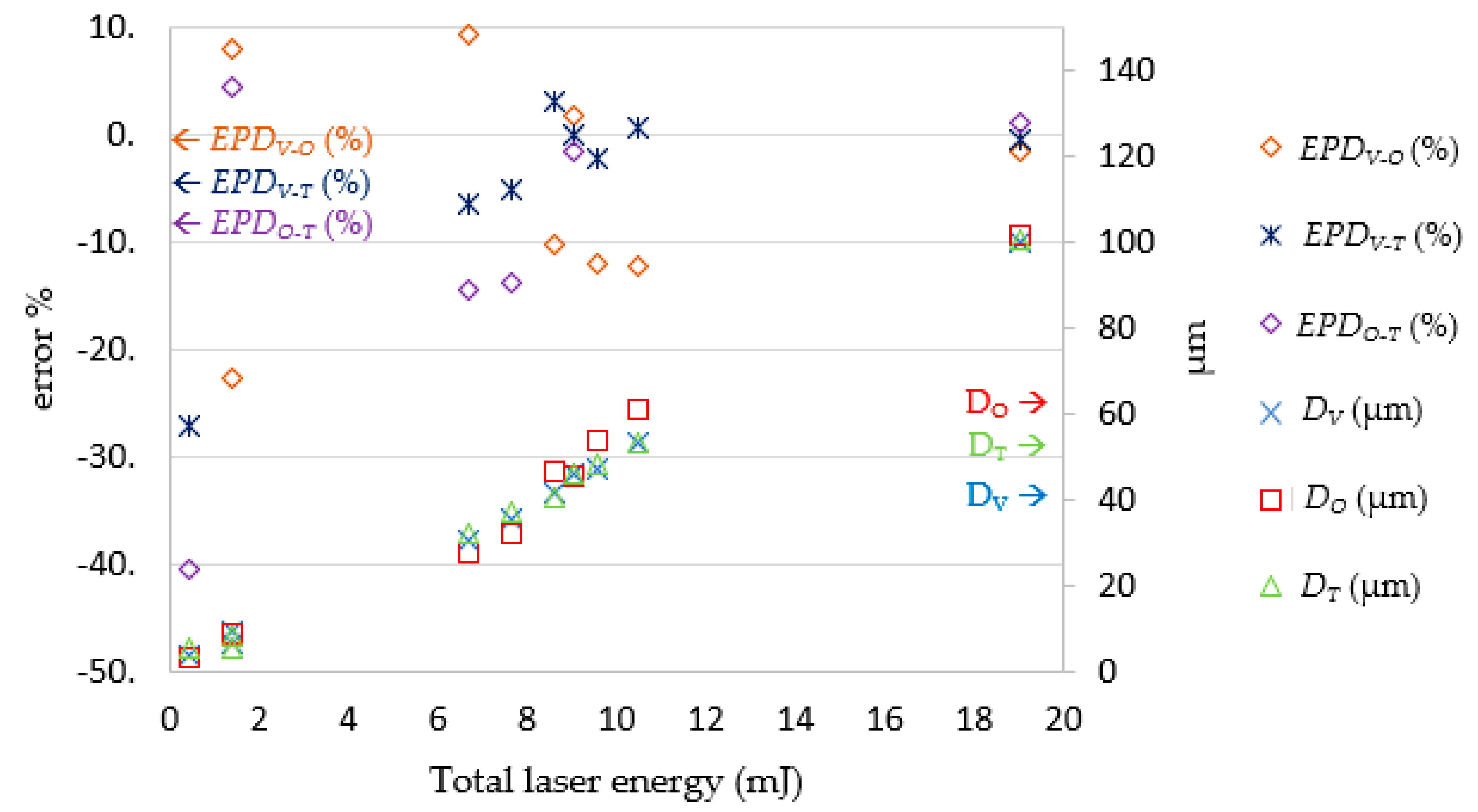
DO. Third, the LPPM-predicted
NP and
EP values were verified by actual laser machining, whereupon the drilled-hole diameters and hole depths,
RV and
DV, respectively, were recorded for verification.
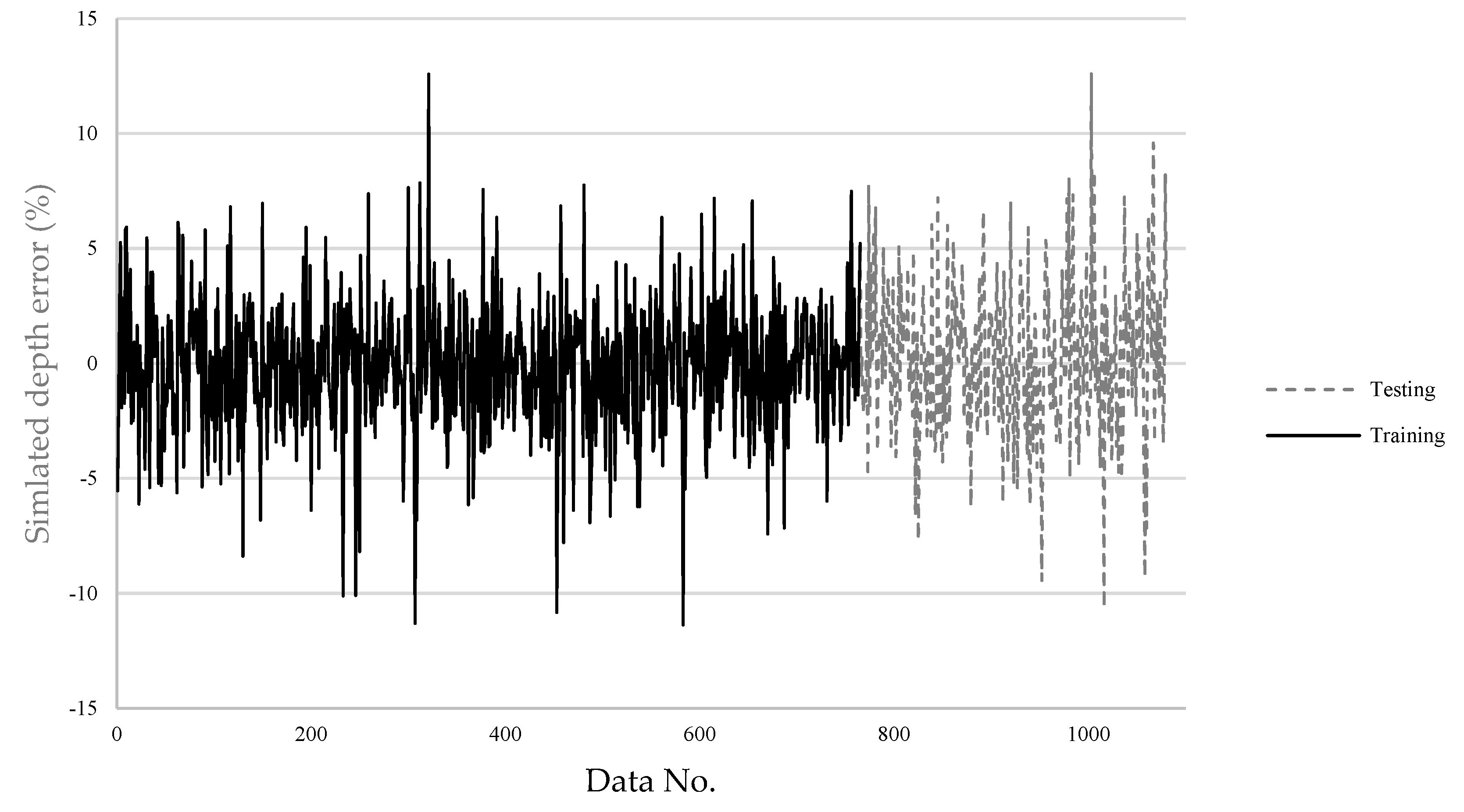
To build the models of LPPM and SLDM, 70% of the 1080 data sets were used for training and 30% were used for testing. The LPPM and SLDM were trained separately.
3.1. LPPM
The LPPM was used to predict the laser pulse energy
EP and number of laser shots
NP required for drilling a hole of a certain size. Therefore, the inputs of the LPPM were hole diameter and depth, and the outputs were laser pulse energy and number of shots. In order to find suitable numbers of hidden layers and neurons of the LPPM, the following trials were conducted and the optimal one was selected. As shown in
Table 3, group A had five hidden layers and the number of neurons in each layer were 4, 6, 8, 10 and 12. Group B had four hidden layers and the number of neurons in each layer were 2, 5, 6 and 8. Group C had three hidden layers and the number of neurons in each layer were 2, 5 and 6. After comparing the results of using three, four, and five hidden layers, a five-layer structure was selected because its error value was the smallest, as shown in
Table 3. In order, the hidden layers of the LPPM contained 4, 6, 8, 10, and 12 neurons. The output layer contained two neurons, and as
Figure 5 shows, the network type was feed-forward, back-propagation.
3.2. LPPM Training with Five-fold Cross-Validation
The 1080 data entries were sorted, randomly numbered, and divided into 5 groups of 216 entries. The group order was changed, and they were fed into the ANN for calculation and analysis.
Table 4 shows that there was no particularly beneficial performance for a given combination, implying that there was no specific pattern to the data.
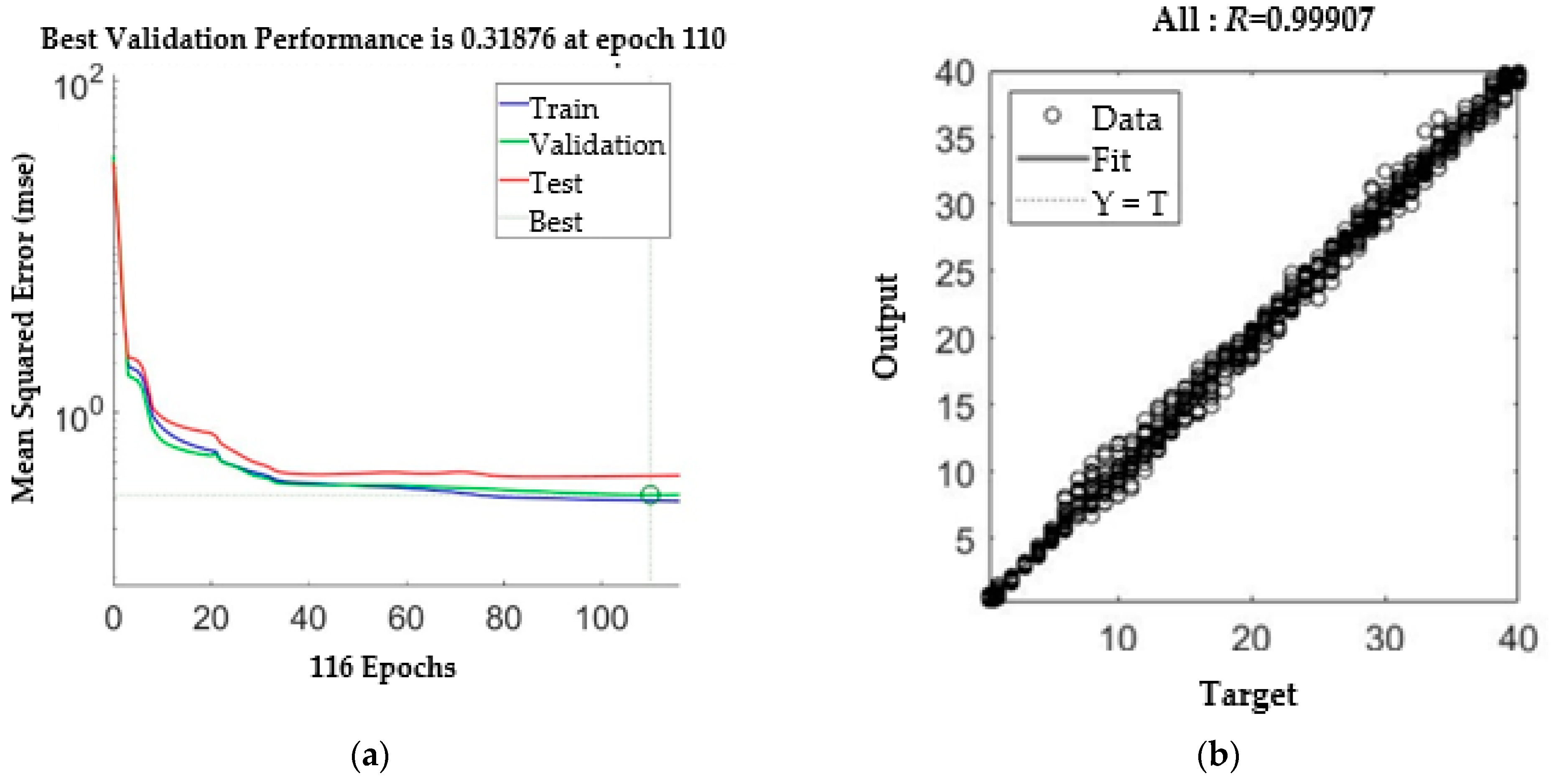
The group with the smallest mean square error (MSE) of approximately 0.325 was selected for use in subsequent experiments. During the training process, and using the groups, the minimal MSE was arrived at on the 110th iteration. The
R value was 0.999, as shown in
Figure 6.
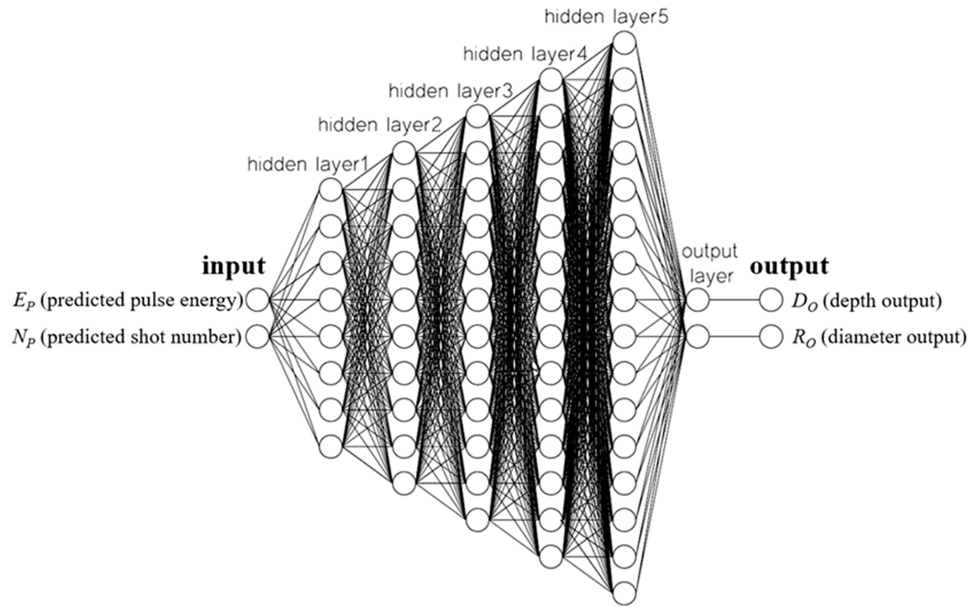
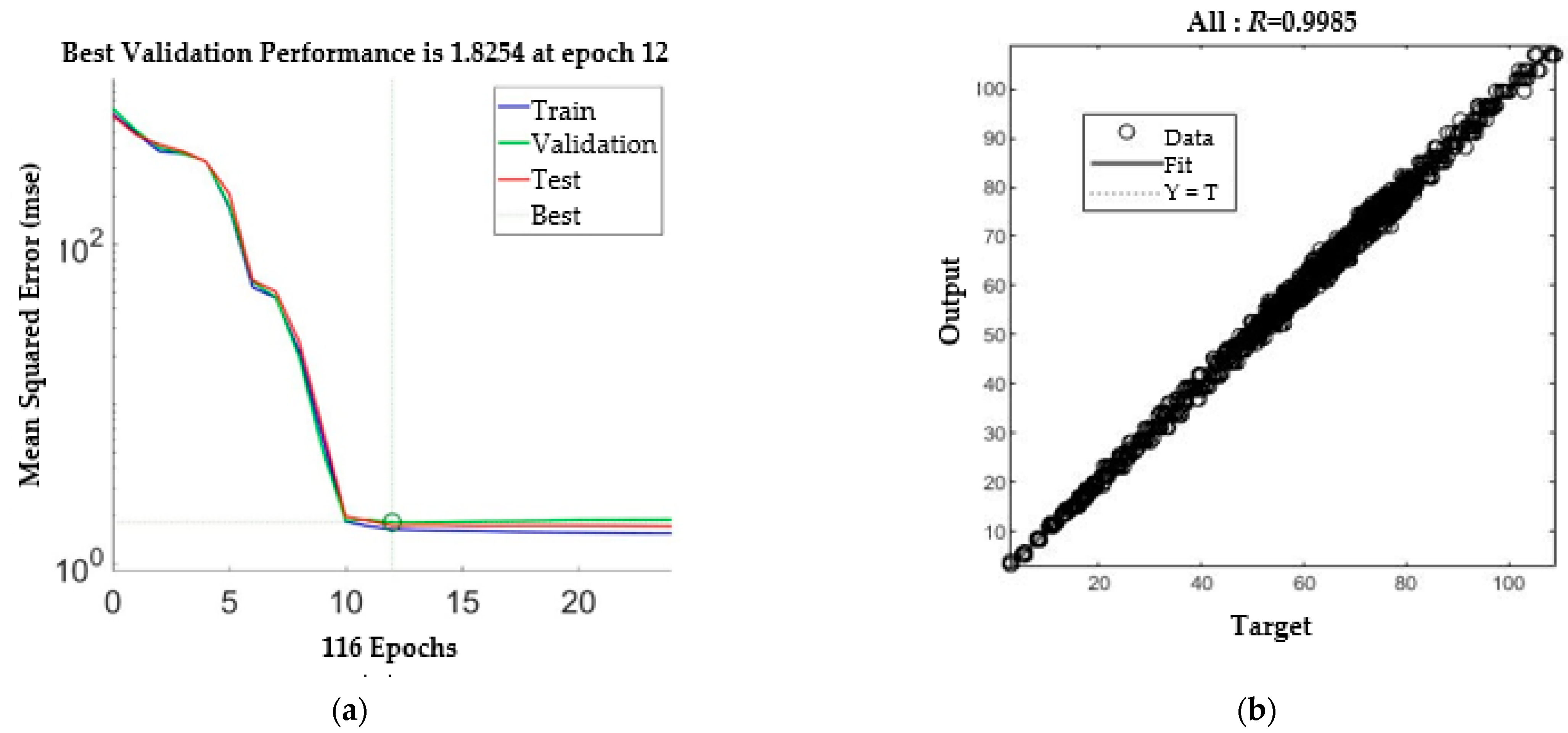
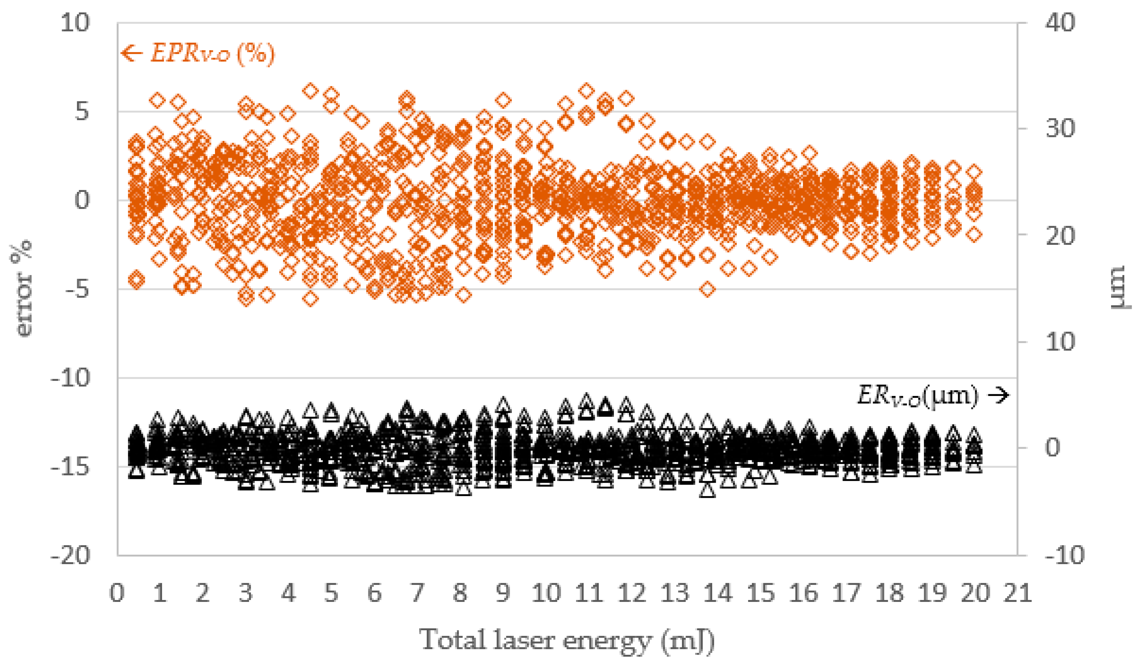
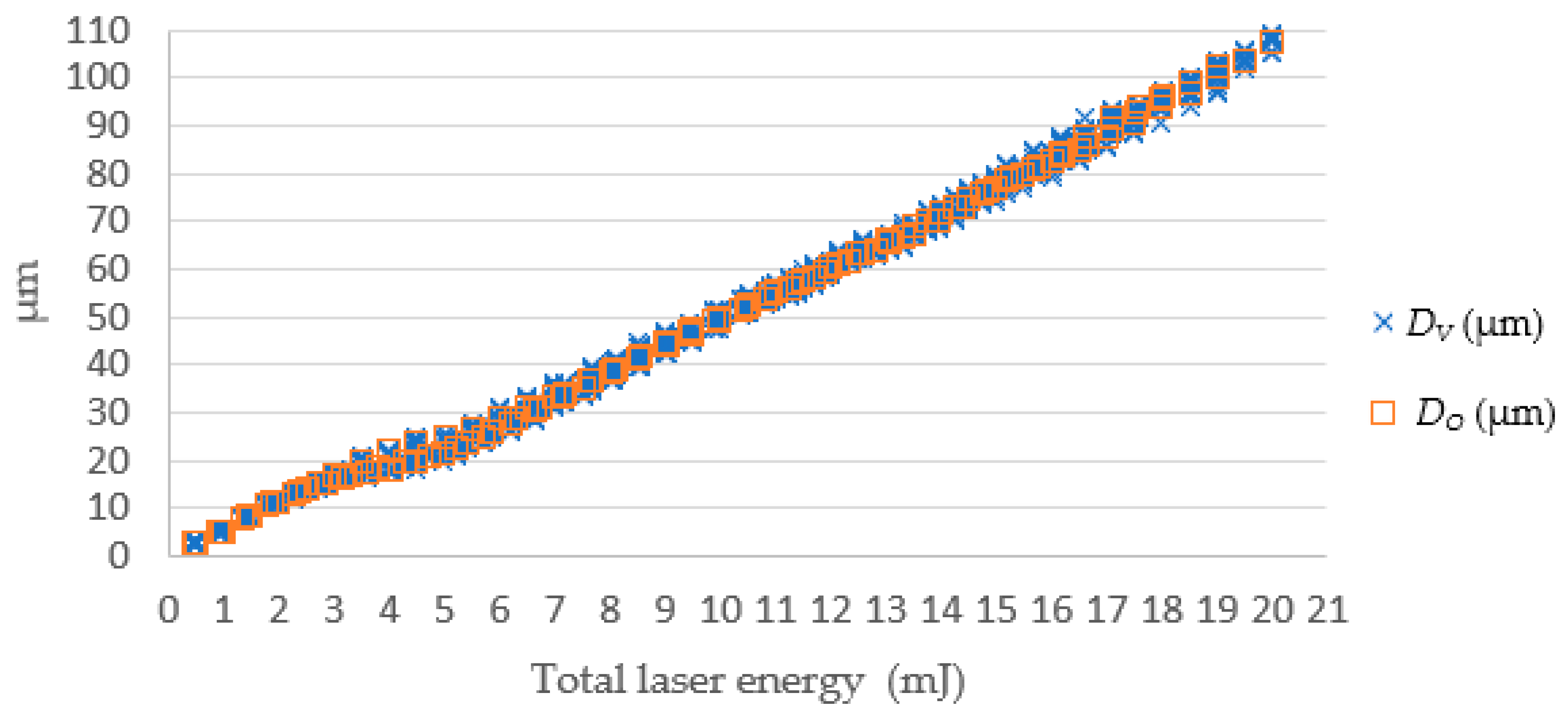
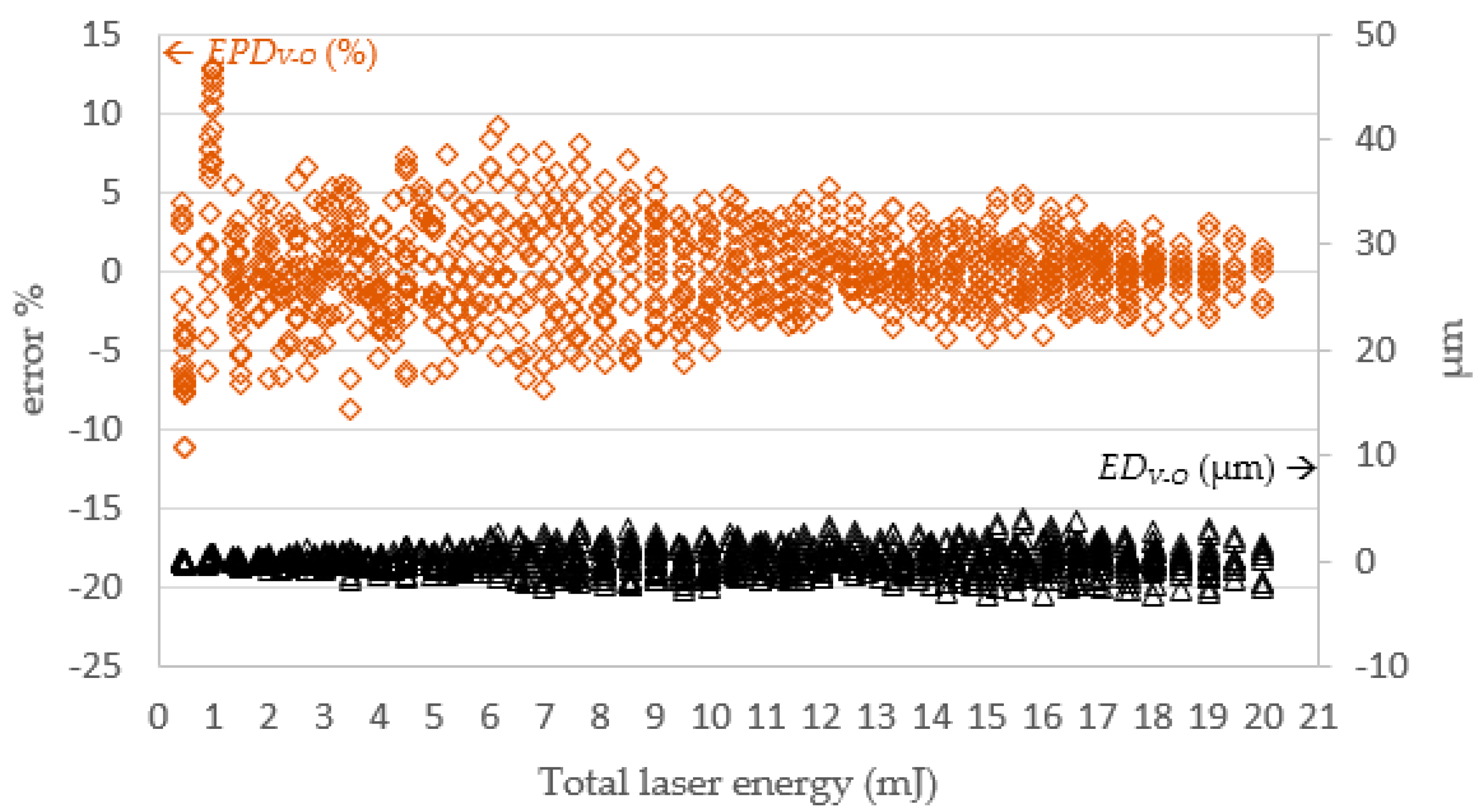
3.3. SLDM
The SLDM was the second ANN and was used to simulate the laser drilling results. The inputs for the SLDM were the number of shots and laser pulse energy, and outputs for the SLDM were hole diameter and depth. Through the same attempt as with the LPPM, the model of SLDM chose five hidden layers, each with 8, 10, 12, 14, and 16 neurons, respectively, as shown in
Figure 7. The MSE obtained after training was 1.8254 and the
R value was 0.9985, as displayed in
Figure 8.


