Abstract
Peatlands are ecosystems of great relevance, because they have an important number of ecological functions that provide many services to mankind. However, studies focusing on plant diversity, addressed from the remote sensing perspective, are still scarce in these environments. In the present study, predictions of vascular plant richness and diversity were performed in three anthropogenic peatlands on Chiloé Island, Chile, using free satellite data from the sensors OLI, ASTER, and MSI. Also, we compared the suitability of these sensors using two modeling methods: random forest (RF) and the generalized linear model (GLM). As predictors for the empirical models, we used the spectral bands, vegetation indices and textural metrics. Variable importance was estimated using recursive feature elimination (RFE). Fourteen out of the 17 predictors chosen by RFE were textural metrics, demonstrating the importance of the spatial context to predict species richness and diversity. Non-significant differences were found between the algorithms; however, the GLM models often showed slightly better results than the RF. Predictions obtained by the different satellite sensors did not show significant differences; nevertheless, the best models were obtained with ASTER (richness: R2 = 0.62 and %RMSE = 17.2, diversity: R2 = 0.71 and %RMSE = 20.2, obtained with RF and GLM respectively), followed by OLI and MSI. Diversity obtained higher accuracies than richness; nonetheless, accurate predictions were achieved for both, demonstrating the potential of free satellite data for the prediction of relevant community characteristics in anthropogenic peatland ecosystems.
Keywords:
fen; wetland; richness; Shannon index; OLI; ASTER; MSI; random forest; generalized linear models; Sphagnum 1. Introduction
Peatlands are wetland ecosystems of great relevance, because they store large amounts of carbon [], regulate the storage and purification of water [], and are a habitat for particular species []. Anthropogenic peatlands emerge when native forests are cut in poorly drained sites, which trigger vegetation succession processes with high moss abundance (from the genus Sphagum []). This moss is currently harvested due to its value as a substrate for horticultural purposes. In this sense, the study of vegetation structure is key to preserving the functions and services that these peatland ecosystems provide to humans [].
Remote sensing is a useful tool for establishing appropriate conservation and management strategies [], allowing the characterization of spatio-temporal dynamics of vegetation, and favoring the acquisition of information on a large scale (particularly in areas of limited access, where field sampling is difficult) []. There are numerous studies that describe different techniques for monitoring wetland vegetation, which have used active sensors such as RADAR (radio detection and ranging) [] or LiDAR (light detection and ranging) [], passive sensors like multispectral [] or hyperspectral [], or data fusion [,]. A detailed review of this subject was presented by Adam et al. [].
Among optical data, free satellite data are particularly important for applications in which there is no clear economic interest. The Landsat Legacy Project is the leading satellite family in the study of vegetation, mainly because it has a very long record (since 1972), providing several applications in the field of plant diversity []. The ASTER sensor is another alternative that has been used to study vegetation and its diversity []; it has been used less frequently, even though it has been in orbit since 1999 (probably because its products were only made freely available in 2016, and it does not have full coverage of the world in each orbit). In 2015 the Sentinel 2A mission was launched, designed especially for the study of vegetation; however, because of its recent launching, it has not been used much. We found only two studies applied on diversity, one to identify dominant species in forests [] and the second to detect and discriminating between grass species C3 and C4 [].
Despite the efforts of the remote sensing community in recent decades, studies in peatland ecosystems are still scarce. Cabezas et al. [] presented the only effort to predict species richness in peatland to date using Landsat 8 imagery. Plant richness has been used in several remote sensing studies as a proxy for α-diversity [,,], which will be referred to as “diversity” in this paper. However, Adam et al. [] argue that understanding the relationship between reflectance, species richness, and species covers is relevant to the ecosystem functioning, which suggests that species richness may not be the best indicator of diversity. A way to include the relative abundance of species is using the Shannon index [], which has already shown good results in remote sensing studies that predict plant diversity [,,]; nevertheless, it has never been mapped in peatlands.
The estimation of plant richness and diversity involves characteristics and challenges that need to be considered. Rocchini et al. [] state that one potential field for refinements is in the model building process, where most of the earlier studies focusing on the estimation of these predictors from remote sensing data often followed simple univariate regression approaches [] or multiple regression models []. Other studies use more complex models, such as partial least squares [], structural equation modeling [], generalized additive models [], and machine learning models (like neural networks [] or random forest (RF) [], among others). It has been proposed that direct application of vegetation indices and simple regression models are not capable of taking full advantage of the information derived from remote sensing data [], for which using non-linear and machine learning models have been implemented, mostly in the last decade []. It is commonly thought that non-linear and machine learning models perform better than linear models in any type of study. However, Lopatin et al. [] demonstrated that this is not necessarily true when predicting species richness. They carried out a comparative study, demonstrating that generalized linear models (GLM) performed better than RF in a complex forest in central Chile, using LiDAR data, given that RF was not able to cope with the asymmetry characteristic of count data (i.e., the number of species), which are discrete and limited to positive values. Therefore, it is necessary to verify if this result can be generalized, or if it was related to the local characteristics of the study.
The aims of this study were: (1) to predict vascular plant richness and diversity in anthropogenic peatlands; (2) to compare RF and GLM algorithms; and (3) to compare free satellite data from the sensors OLI, ASTER, and MSI on board satellite platforms Landsat 8, Terra, and Sentinel 2A, respectively.
2. Materials and Methods
2.1. Study Area
The study area is located in northern Chiloé Island, commune of Ancud, Los Lagos Region, Chile (41°52′40″S, 73°40′00″W) (Figure 1). It specifically corresponds to three anthropogenic peatlands, whose origins are in the logging and/or burning of native forest (which results in bare soil with poor drainage areas, generating flooding conditions that allow the colonization and settlement of Sphagnum moss species []).
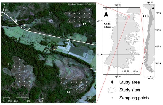
Figure 1.
Location of the study sites in the north of Chiloé Island in southern Chile. Polygons represent the peatlands P1, P2 and P3. White squares represent the location of the sampling plots.
The climate is temperate with oceanic influence, with a dry period in summer. Annual precipitation is about 2100 mm, with mean annual temperatures of ~10 °C.
The three study peatlands are located at the Senda Darwin Biological Station (P2) and its surroundings (Figure 1), whose extensions are 10.5, 5.6, and 6.2 ha for P1, P2, and P3, respectively. Currently, the three peatlands do not present significant human pressure, allowing the successional development of vascular plants over the Sphagnum layer.
The three peatlands have the same dominant species, which are Baccharis patagonica, Gaultheria mucronata, Myrteola numularia, and Sticherus cryptocarpus (a full description of species composition and abundance is presented in Table S1). In addition, there is an important area dominated by reed species (Juncus procerus, Juncus planifolius, and Juncus stipulatus) and several species of ferns, dominated by the genus Blechnum (B. chilensis and B. penna-marina, among others). In spite of the species shared between peatlands, these can be differentiated in their horizontal structure, since their spatial arrangement and mean cover vary from one another. Peatland P1 has a structure dominated by open scrubs, allowing the establishment of numerous herbaceous species (most of them Gramineae) over Sphagnum, and reed species in flooded areas. Peatland P2 is dominated by dense shrubs, with a lesser number of herbs species. Reeds are still present in flooded areas where Sphagnum remains exposed. Peatland P3 has a matrix dominated by dense scrubs, with the same species mentioned for P2 but with the presence of Philesia magellanica (in addition to the presence of tree species), foregrounding the presence of the endangered Pilgerodendron uviferum.
2.2. Ground Data
A systematic sampling of vascular plant richness (expressed as the number of species in a given area or a given sample) was conducted to adequately represent the variability of the ecosystem, due to the high spatial heterogeneity of peatlands []. For this task, sampling points were located in a regular grid of 60 m in each peatland, to adjust the sampling points with the spatial resolution of Landsat 8 (30 m). This implied that 15 sampling points were located in each peatland, obtaining a total of 45 observations. Each plot consists in square plots of 2 m × 2 m, where the species occurrence and cover were registered []. The vegetation assessments were conducted in two field campaigns: during January 2014 for P2, and during January 2016 for P1 and P3 (Figure 1).
Finally, we obtained for each plot the species richness (species count) and diversity, which we estimated using the Shannon index []. This index is one of the most popular plant diversity indexes used in ecological studies [], and can be calculated as , where Pi is the relative proportion of species i. Foody and Cutler [] point out the superiority of that index over the richness, to reflect the structural variability of a landscape (since it allows a better representation of the dominant composition, and hence the dominant structure of a plant community).
2.3. Remote Sensing Predictors
Models were built with free available satellite data from three sensors: Operational Land Imager (OLI), Advanced Spaceborne Thermal Emission and Reflection (ASTER), and Multi Spectral Instrument (MSI). Acquisition dates of scenes were defined according to the field campaigns date. For OLI, the dates were 24 December 2013, and 6 January 2016. Surface reflectance at 30 m spatial resolution was obtained from The Climate Data Record (CDR). ASTER scenes were obtained on 23 September 2013 and 31 January 2016. Surface reflectance at 15 m spatial resolution was obtained from the ASTER 7XT products. MSI data were obtained only for 5 January 2016, because it has only been operational since mid-2015). Top of Atmosphere reflectance at 10 m spatial resolution was obtained for the visible spectrum and one near infrared band (NIR), and at 20 m resolution in four NIR bands and two Shortwave Infrared bands (SWIR). Data were acquired from the Level 1C product, and the Dark Object Subtraction (DOS) atmospheric correction was applied to derive Surface reflectance [].
Model predictors were obtained from all available bands of the three sensors. From these reflectance ranges, common vegetation indices (VI) used in wetland studies were computed (see Table 1). Furthermore, texture predictors were obtained from spectral bands and VI, which were divided in first and second order predictors, following Mairota et al. []. The first order predictors were the median and the standard deviation of pixels obtained from a 3 × 3 moving window, computed using focal statistics tools from ArcGIS 10.3 (ESRI, Redlands, CA, USA). The second order predictors were obtained using the gray-level co-occurrence matrix (GLCM) [], namely the mean, variance, homogeneity, contrast, correlation, second moment, entropy, and dissimilarity. A 3 × 3 moving window was considered, using ENVI 5.1 (Exelis Visual Information Solutions, Boulder, CO, USA).

Table 1.
Spectral predictors obtained from OLI, ASTER, and MSI satellite products.
Finally, three sets of predictors were obtained, with a total of 148, 360, and 724 predictors for the OLI, ASTER, and MSI models, respectively. Reflectance values at the plot locations were obtained by bilinear interpolation [].
2.4. Statistical Models
Species richness was modeled using two approaches: random forest (RF), and generalized linear models (GLM).
According to Lopatin et al. [], the processing of data using GLM can be subdivided into three steps:
- Identify the proper model family to deal with the statistical properties of the observed variables. To predict species richness, we compared the normalized quantile-plots of the residuals of several GLMs, using the model families which are generally recommended for count data: Poisson, Quasi-Poisson, and negative binomial. All models tested were set with log-link functions. To predict the diversity, we tested model families (recommended for continuous positive data) as Gamma with inverse, identity, and log-link functions. Likewise, we tested less adequate Gaussian error distribution with log-link function. In all cases we tested the models using the best (only one) predictor, ranked by recursive feature elimination (RFE; see below). By the shape of the normalized quantile-plots of the residuals, we selected the Poisson error distribution with a log-link function for the species richness models, while the Gaussian error distribution with log-link function was selected for the prediction of diversity.
- Select the subset of predictors for each model. As GLMs cannot cope with multi-collinearity among independent predictors, a selection and ranking of the most important predictors was performed by the recursive feature elimination (RFE) algorithm []. This algorithm operates based in an iterative procedure, in which one predictor at a time is eliminated and ranked by its importance. We used random forest as the kernel. RFE was implemented using a leave-one-out cross validation procedure to acquire the RMSE and the number and importance of predictors. Models were selected based on a tradeoff between a low RMSE and a low number of predictors. In addition, we followed the recommendations of Hair et al. [], who state that the number of observations should not be less than 5 per predictor, and ideally should be between 15 and 20.
- With the first subset obtained, the correlation between these predictors was assessed using the Pearson correlation coefficient (r), selecting the pairs of predictors with r ≥ ǀ0.6ǀ and eliminating, one by one, the least important predictors according to the RFE ranking. This process was carried out independently for each sensor model, so the models could be compared.
- Select the final model. The final number of predictors were determined by calculating several models and adding a single predictor in each run (starting with the most important predictor according to RFE). The best number of predictors was assessed by comparing the Akaike information criterion (AIC) and deviance []. We selected the model using three predictors.
The ensemble regression tree method RF [] has been reported to be an efficient predictive approach, especially when the number of observations is comparatively low compared to the number of predictors []. The algorithm requires that two parameters be set: (1) mtry, the number of predictors performing the data partitioning at each node; and (2) ntree, the total number of trees to be grown in the model run. The ntree parameter was set to 500, following the recommendations in the literature [], while mtry was tuned for each model. All statistical processes were carried using R (packages randomForest [] and Caret []). Here, we also use the RFE-ranked predictors to find the best set of predictors. As in the GLM models, we added a single predictor at the time to find the best model per sensor. The best models were selected by the percentage of explained variance.
To check the statistical assumptions of the models, we applied a Shapiro-Wilk [] test to the residuals and the Moran test to assess the spatial auto-correlation [], discarding those models that did not pass both tests.
2.5. Model Validation
For validation purposes, we followed the recommendations of Lopatin et al. [], where the final RF and GLM models were embedded in a bootstrap procedure with 500 iterations. In each bootstrap iteration we drew 45 times, with replacements from the 45 available samples. In this procedure, on average, 36.8% of the total number of samples (~28 samples) were not drawn, and were used as samples for the independent validation []. The model performances of RF and GLM were compared, based on differences in the squared Pearson correlation coefficient (R²), normalized root square error (%RMSE), bias (measured as one minus the slope of a regression, without intercept of the predicted versus observed values), and a final model selected. We tested for significance differences (α = 0.05) between algorithms and sensors by applying a one-sided bootstrap test []. First, we obtained the median values of the previous bootstrap accuracies (R², %RMSE and bias), described above. Using these values as a reference, we selected which algorithm performed accurately for each sensor. Second, we embedded the models in another bootstrap, where in each iteration the R² of the ‘better’ models were subtracted by the R² of the ‘worst’ model, and the other way around for %RMSE and bias (assuming that the ‘better’ model will have higher R² and lower errors and bias). From these distributions, a one-sided test was performed to test if the differences between GLM and RF were larger than zero (based on 500 bootstrap samples). The same procedure was applied to define significant differences between sensors (using the best algorithm in each sensor).
2.6. Predictive Species Map
The final step of the procedure consisted in obtaining the richness and diversity maps, which was done using the best models obtained in each case. The maps were computed based on 500 iterations from the bootstrap, using the best selected models in each iteration. The predictors used to generate the models were spatially explicit, allowing the extrapolation (and prediction) of areas that were not covered by the pixels used to build the models, which correspond to the field samples. With that procedure 500 predictive maps were obtained, and we report maps of the median values and the coefficient of variation (CV, given in %) values for the species richness and diversity, to account for stability in predictions within each pixel. The predictions were made solely within the limits of the study of peatlands, to avoid predictions beyond the range of the model.
3. Results
3.1. Model Performance
By applying RFE, we obtained the importance and the optimal number of predictors for each model. According to Hair et al. [], and considering the number of the observation in our study (n = 45), the maximum number of predictors for each model was 3. Table 2 shows the predictors included in the final models for predicting plant richness and diversity.
Table 2.
Predictors selected in the final models. The predictors used in each model are marked with an x and ordered importance according to recursive feature elimination (RFE). Abbreviations of predictors are presented in Table 1. The numbers in the subscript correspond to the central wavelength of the sensor band (see Table S2).
The validation metrics R2, %RMSE, and bias, obtained from the 500 bootstrap, showed no significant differences between GLM and RF for species richness and diversity (Figure 2); but, in most cases, GLM models showed higher accuracies using fewer predictors, except for species richness prediction obtained with MSI (Table 2).
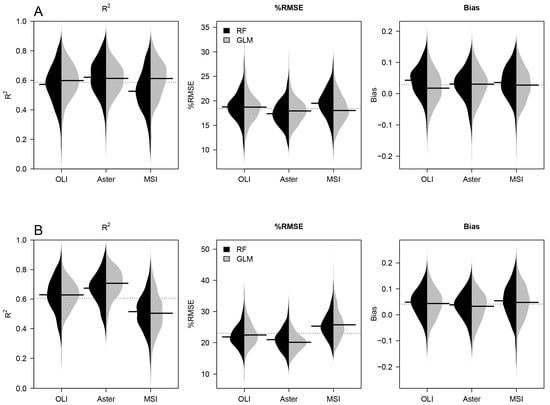
Figure 2.
Model accuracies of random forest (RF) (black plots) and generalized linear model (GLM) (gray plots) in terms of R2, RMSE, and bias for richness (panel A) and diversity (B). Beanplot display distribution of results for the 500 bootstrap runs. Black horizontal lines represent the median of the distributions.
Non-significant differences were found between algorithms and sensors; however, higher accuracies were obtained with ASTER for species richness performed with RF (R2 = 0.62 and %RMSE = 17.2% for the median bootstrap value) and for diversity performed with GLM (R2 of 0.71 and %RMSE of 20.2% for the median bootstrap value) (Table 3). OLI obtained a similar performance for predicting species richness with GLM (R2 = 0.59 and %RMSE = 18.3% for the median of bootstrap), but a slightly lower for predicting diversity with GLM (R2 = 0.63 and %RMSE = 22.8% for the median bootstrap value). MSI obtained similar prediction of species richness with GLM (R2 = 0.60 and %RMSE = 18.3% for the median bootstrap value), but inferior prediction of diversity using RF. Predictions of diversity obtained higher accuracy than species richness in terms of R2, but not in terms of %RMSE and Bias (Table 3), showing a systematic error in the diversity predictions.
Table 3.
Median bootstrap model accuracies per sensor.
3.2. Prediction Map
Predictive maps of richness and the Shannon index, and their corresponding coefficient of variation, are shown in Figure 3 and Figure 4, respectively. No spatial autocorrelation was found for the residuals of the models (Moran: I = −0.053, P = 0.68 for species richness and I = −0.051, P = 0.66 for diversity), demonstrating robust spatial predictions. The predictive map of species richness shows values ranging between 6 and 13 species, distributed evenly along the three peatlands, with most of the values around 6 and 10 species and maximum values located in the border of the peatlands. The map of CV represents the stability of the predictions, with maximum values around 14% in a few pixels, and most of them <9% (Figure 3).
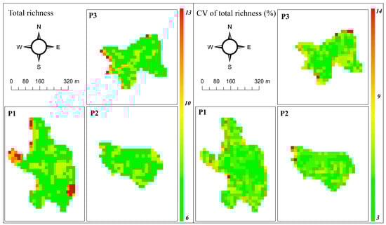
Figure 3.
Species richness prediction (left) and coefficient of variation (right) maps using ASTER sensor data and RF. The Predicted values represent the median of 500 bootstrap runs in each pixel.
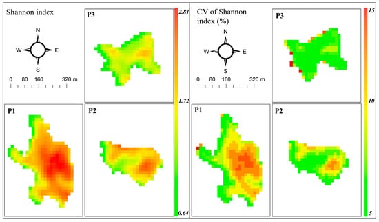
Figure 4.
Diversity prediction (left) and coefficient of variation (right) maps using ASTER data and GLM. Predicted values represent the median of 500 bootstrap runs in each pixel.
The predictive maps of diversity show values ranging between 0.64 and 2.81, with the highest values in peatland P1, followed by P2 and P3 (Figure 4). The high values correspond to areas where shrubs are more sparsely distributed and where Sphagnum remains freely exposed, allowing the establishment of numerous herbaceous species. The map of CV shows values <15%, with higher variability in areas with a high level of the Shannon index (Figure 4).
4. Discussion
4.1. Selected Predictors and Their Ecological Implications
Most selected predictors for modeling plant richness in peatland ecosystems had the influence of the infrared electromagnetic spectrum, which is a wavelength area often defined as the most relevant to study the differences in vegetation structures [,]. In the NIR region, high levels of reflectance are present, due to the cellular structure of leaves that reflect a great part of the incident energy, and by canopy structural traits, such as leaf area and angle [], that can differentiate between species compositions or plant strategies [] related to diversity. Meanwhile, in the SWIR region there is a low reflection in specific regions of the spectrum, where water molecules within cells absorb most of the incident energy []. The visible spectrum, generally dominated by the absorption of pigments and canopy structures, usually has less variability among plant species, as compared to infrared spectrum [,].
Regarding the selected predictors, most of them (14 out of 17) were textural predictors derived from GLCM or standard deviation (Table 2). The spectral heterogeneity has been defined as the most important factor that explains plant richness [] and plant diversity []. This statement was based on the spectral variation hypothesis, which states that a higher spectral heterogeneity shows a positive correlation with species richness [,]. Theoretical and empirical studies suggest that the diversity of a particular site is strongly influenced by and positively correlated with its environmental heterogeneity []. More complex environments can host a greater number of ecological niches, which in turn can be colonized and inhabited by a larger number of species. In our study, developed at a local scale, this phenomenon was well captured by the spectral heterogeneity contained in the textural metrics (derived from spectral information). Nevertheless, recent efforts have proven that this hypothesis may not hold areas across landscapes with coarser resolution [].
4.2. Satellite Sensor Comparison
Similar predictions for species richness and diversity were obtained for the three sensors, with greater discrepancy in diversity predictions (Figure 2). The non-significant differences was likely related to a similar spatial resolution (ranging from 10 to 30 m), and to the spectral capabilities of sensors to provide NIR information, which has demonstrated to be relevant in α-diversity studies [,].
Considering this, it is expected that MSI should provide the best predictions of richness and diversity because of its more detailed spectral representation of the NIR region, including 5 bands. We found something different, which may have been caused by the following factor: the use of a January 2016 image for representing the field samples of January 2014 in Peatland 2, due to the lack MSI scenes before 2015. That mismatching between field samples and satellite observations could be the main reason for the poor performance of MSI. This is supported by Bradley [], who mentioned that, ideally, acquisition time should be at the same time as field samples extraction (the method of atmospheric correction applied to MSI information), since DOS has demonstrated to have poor performances in several applications (e.g., []). In this sense, ASTER and OLI products have implemented complex and validated atmospheric correction algorithms, which can provide a more reliable estimation of surface reflectance (the spatial resolution of NIR bands could have played a role as well, especially in peatlands where the community gradient and soil chemical compositions may change drastically over distances of a few meters []). Here we obtained better predictions with the ASTER sensor (the one with finer spatial resolution (15 m)) as compared to MSI (20 m) and OLI (30 m), allowing a better representation of ecosystem variability, in terms of composition and dominance of species []. This is consistent with the results of other studies, where the NIR spectrum region was selected as the most relevant predictor using a hyperspectral sensor to separate species in a mangrove ecosystem, where water and vegetation strongly interact []. The use of ASTER sensor in α-diversity predictions was already been reported by Feilhauer and Schmidtlein [], who obtained similar results in a walnut-fruit forest for species richness (R2 = 0.51) and diversity (R2 = 0.61).
Regarding the textural metrics, Laurin et al. [] in the Gola Rainforest National Park, obtained good predictions (R2 = 0.84) using these type of metrics to estimate diversity based on hyperspectral data. Species richness predictions, using textural predictors, were reported by Cabezas et al. [] in an anthropogenic peatland divided into two zones with different types of management: productive (with Sphagnum extraction) and conservation (corresponding to peatland P2 in this study). In summary, spatial resolution of the scenes seems to be important for the analysis, especially in peatlands. Rocchini et al. [] point out that ideally the size of the pixel should be at least the same size as the sampling unit, especially when spectral heterogeneity is computed to estimate the local diversity of species, as in this study. Nevertheless, when pixel size has a very small dimension (1–5 m), the shadows can create a high level of spatial heterogeneity that can lead to producing more noise rather than adding relevant information []. In addition, Rocchini et al. [] mentioned that coarse spatial resolutions can affect the representation of actual heterogeneity due to a smoothing process that makes it difficult to detect patterns that exist at a finer scale. Hence, this trade-off between noises caused by high resolution and the information loss caused by low resolution must be taken into account.
Nonetheless, in this study the moving window of 3 × 3 pixels was considered to compute the textural predictors, regardless of the spatial resolution of each sensor. Therefore, the smoothing effect differs among sensors, and thus could possibly affect the representation of actual heterogeneity of the ecosystems, consequently underestimating the environmental gradient at low resolutions. However, on the three-pixel scale considered, similar accuracies were obtained by the different modeling approaches, which may imply that the spatial difference (10–30 m) does not result in a significant difference in the acquisition of textural information in such highly heterogeneous environments (where medium-resolution satellites may only account for general patterns).
4.3. Model Comparisons
The slightly better performance (though not significant) of GLM in species richness modeling could be due to its ability to handle count data, where the error has a non-symmetrical distribution []. In our particular case, the Poisson distribution was the most appropriate to represent the error distribution, agreeing with other studies [].
Machine-learning methods such as RF are popular among modelers because they are described as non-parametric, because it is usually assumed that there are no requirements concerning the error distribution. Nevertheless, this is not true for RF, which either fits standard linear (Gaussian) regressions for tree nodes or is based on measures for node impurity, such as the sum of squared deviations from the mean []. But, it is true that in several cases they have proven to be more accurate than parametric approaches with easier tuning procedures. Despite these advantages, their predictions are often difficult to follow, compared to parametric approaches such as GLM []. Another issue with RF is that the application of sub-sampling in the algorithm can result in an increment of the variance, especially when the number of samples is small []. This can turn into a major problem in the validation process, when the bootstrap method is implemented and sub-samples are chosen, reducing the input observations used in the model. In spite of these limitations, studies using RF to predict species richness obtained accurate predictions with similar field samples as the one used in this study [,], and demonstrated to be an important tool for modeling α-diversity. This study shows that both GLM and RF are valid methods for predicting α-diversity with similar performance; nonetheless, according to Latifi et al. [] and Lopatin et al. [], GLM proved to be a more parsimonious approach, since it was easier to interpret, required less computation time, and fewer predictors.
5. Conclusions
Accurate predictions of α-diversity were obtained in anthropogenic peatlands from data of three medium-resolution sensors (OLI, ASTER, and MSI), using the random forest (RF) and generalized linear model (GLM) approaches. Predictions of vascular plant richness were obtained with an acceptable level of accuracy, and similar results were obtained for plant diversity, demonstrating the capability of sensors to estimate α-diversity.
In spite of the non-significant differences between algorithms and sensors, ASTER was able to provide the most accurate models for both species richness and diversity, probably due to its spatial resolution in the NIR band. The comparison between RF and GLM modeling approaches showed no significant differences either, but slightly better results were often obtained with GLM, which is easier to understand and provides a more parsimonious prediction with fewer predictors. Most of the selected predictors were derived from the computation of textural variables. The inclusion of the spatial context represented by the textural metrics was an important feature in modeling α-diversity.
Free satellite data have proven to be helpful for modeling α-diversity in anthropogenic peatlands, which are ecosystems of great relevance (both locally and globally).
Supplementary Materials
The following are available online at www.mdpi.com/2072-4292/9/7/681/s1, Table S1: Species cover by peatland, Table S2: Spectral resolution of sensors. The sensor bands are divided by spectral range, where NIR is near infrared and SWIR is short wave infrared.
Acknowledgments
The authors thank FONDECYT Grant N 1130935 and Project CONICYT/FONDAP/1511000.
Author Contributions
Mauricio Galleguillos, and Jorge Perez-Quezada conceived and designed the experiments; Ivan Castillo, Mauricio Galleguillos, Jorge Perez-Quezada, and Javier Lopatin performed the experiments; Ivan Castillo and Javier Lopatin analyzed the data; Javier Lopatin and Mauricio Galleguillos contributed materials/analysis tools; Ivan Castillo, Mauricio Galleguillos, Javier Lopatin, and Jorge Perez-Quezada wrote the paper.
Conflicts of Interest
The authors declare no conflict of interest.
References
- Zedler, J.B.; Kercher, S. Wetland resources: Status, trends, ecosystem services, and restorability. Annu. Rev. Environ. Resour. 2005, 30, 39–74. [Google Scholar] [CrossRef]
- Bullock, A.; Acreman, M. The role of wetlands in the hydrological cycle. Hydrol. Earth Syst. Sci. 2003, 7, 358–389. [Google Scholar] [CrossRef]
- Keddy, P.A. Wetland Ecology: Principles and Conservation, 2nd ed.; Cambridge University Press: New York, NY, USA, 2010; p. 497. [Google Scholar]
- Díaz, M.F.; Bigelow, S.; Armesto, J.J. Alteration of the hydrologic cycle due to forest clearing and its consequences for rainforest succession. For. Ecol. Manag. 2007, 244, 32–40. [Google Scholar] [CrossRef]
- Duffy, E. Why biodiversity is important to the functioning of real-world ecosystems. Front. Ecol. Environ. 2009, 7, 437–444. [Google Scholar] [CrossRef]
- Turner, W. Sensing biodiversity. Science 2014, 346, 301–302. [Google Scholar] [CrossRef] [PubMed]
- Lee, K.H.; Lunetta, R.S. Wetland detection methods. In Wetland and Environmental Application of GIS, 1st ed.; Lyon, J.G., McCarthy, J., Eds.; Lewis Publishers: New York, NY, USA, 1996; pp. 249–284. [Google Scholar]
- Evans, T.L.; Costa, M.; Tomas, W.M.; Camilo, A.R. Large-scale habitat mapping of the Brazilian Pantanal wetland: A synthetic aperture radar approach. Remote Sens. Environ. 2014, 155, 89–108. [Google Scholar] [CrossRef]
- Luo, S.; Wang, C.; Pan, F.; Xi, X.; Li, G.; Nie, S. Estimation of wetland vegetation height and leaf area index using airborne laser scanning data. Ecol. Indic. 2015, 48, 550–559. [Google Scholar] [CrossRef]
- Cole, B.; McMorrow, J.; Evans, M. Spectral monitoring of moorland plant phenology to identify a temporal window for hyperspectral remote sensing of peatland. ISPRS J. Photogramm. Remote Sens. 2014, 90, 49–58. [Google Scholar] [CrossRef]
- Cole, B.; McMorrow, J.; Evans, M. Empirical modeling of vegetation abundance from airborne hyperspectral data for upland peatland restoration monitoring. Remote Sens. 2014, 6, 716–739. [Google Scholar] [CrossRef]
- Aslan, A.; Rahman, A.; Warren, M.; Robeson, S. Mapping spatial distribution and biomass of coastal wetland vegetation in Indonesian Papua by combining active and passive remotely. Remote Sens. Environ. 2016, 183, 65–81. [Google Scholar] [CrossRef]
- Dabrowska-Zielinska, K.; Budzynska, M.; Tomaszewska, M.; Bartold, M.; Gatkowska, M.; Malek, I.; Turlej, K.; Napiorkowska, M. Monitoring wetlands ecosystems using ALOS PALSAR (L-Band, HV) supplemented by optical data: A case study of Biebrza Wetlands in Northeast Poland. Remote Sens. 2014, 6, 1605–1633. [Google Scholar] [CrossRef]
- Adam, E.; Mutanga, O.; Rugege, D. Multispectral and hyperspectral remote sensing for identification and mapping of wetland vegetation: A review. Wetl. Ecol. Manag. 2009, 18, 281–296. [Google Scholar] [CrossRef]
- Savage, S.L.; Lawrence, R.L.; Squires, J.R. Predicting relative species composition within mixed conifer forest pixels using zero-inflated models and Landsat imagery. Remote Sens. Environ. 2015, 171, 326–336. [Google Scholar] [CrossRef]
- Mutowo, G.; Murwira, A. Relationship between remotely sensed variables and tree species diversity in savanna woodlands of Southern Africa. Int. J. Remote Sens. 2012, 33, 6378–6402. [Google Scholar] [CrossRef]
- Laurin, G.; Puletti, N.; Hawthorne, W.; Liesenberg, V.; Corona, P.; Papale, D.; Chen, Q.; Valentini, R. Discrimination of tropical forest types, dominant species, and mapping of functional guilds by hyperspectral and simulated multispectral Sentinel-2 data. Remote Sens. Environ. 2016, 176, 163–176. [Google Scholar] [CrossRef]
- Shoko, C.; Mutanga, O. Examining the strength of the newly-launched Sentinel 2 MSI sensor in detecting and discriminating subtle differences between C3 and C4 grass species. ISPRS J. Photogramm. Remote Sens. 2017, 129, 32–40. [Google Scholar] [CrossRef]
- Cabezas, J.; Galleguillos, M.; Perez–Quezada, J.F. Predicting vascular plant richness in a heterogeneous wetland using spectral and textural features and a random forest algorithm. IEEE Geosci. Remote Sens. Lett. 2016, 13, 646–650. [Google Scholar] [CrossRef]
- Lopatin, J.; Galleguillos, M.; Fassnacht, F.E.; Ceballos, A.; Hernández, J. Using a multistructural object–based LiDAR approach to estimate vascular plant richness in Mediterranean forests with complex structure. IEEE Geosci. Remote Sens. Lett. 2015, 12, 1008–1012. [Google Scholar] [CrossRef]
- Latifi, H.; Fassnacht, F.; Koch, B. Forest structure modeling with combined airborne hyperspectral and LiDAR data. Remote Sens. Environ. 2012, 121, 10–25. [Google Scholar] [CrossRef]
- Shannon, C. A mathematical theory of communication. Bell Syst. Tech. J. 1948, 27, 379–423. [Google Scholar] [CrossRef]
- Nagendra, H. Opposite trends in response for the Shannon and Simpson indices for landscape diversity. Appl. Geogr. 2002, 22, 175–186. [Google Scholar] [CrossRef]
- Laurin, G.; Chan, J.; Chen, Q.; Lindsell, J.; Coomes, D.; Guerriero, L.; del Frate, F.; Miglietta, F.; Valentini, R. Biodiversity Mapping in a Tropical West African Forest with Airborne Hyperspectral Data. PLoS ONE 2014, 9, e97910. [Google Scholar]
- Rocchini, D.; Marcantonio, M.; Riccota, C. Measuring Rao’s Q diversity index from remote sensing: An open source solution. Ecol. Indic. 2017, 72, 234–238. [Google Scholar] [CrossRef]
- Rocchini, D.; Balkenhol, N.; Carter, G.A.; Foody, G.M.; Gillespie, T.W.; He, K.S.; Kark, S.; Levin, N.; Lucas, K.; Luoto, M.; et al. Remotely sensed spectral heterogeneity as a proxy of species diversity: Recent advances and open challenges. Ecol. Inform. 2010, 5, 318–329. [Google Scholar] [CrossRef]
- Oldeland, J.; Wesuls, D.; Rocchini, D.; Schmidt, M.; Jurgens, N. Does using species abundance data improve estimates of species diversity from remotely sensed spectral heterogeneity? Ecol. Indic. 2010, 10, 390–396. [Google Scholar] [CrossRef]
- Ceballos, A.; Hernández, J.; Corvalán, P.; Galleguillos, M. Comparison of airborne LiDAR and satellite hyperspectral remote sensing to estimate vascular plant richness in deciduous mediterranean forests of central Chile. Remote Sens. 2015, 7, 2692–2714. [Google Scholar] [CrossRef]
- Feilhauer, H.; Schmidtlein, S. Mapping continuous fields of forest alpha and beta diversity. Appl. Veg. Sci. 2009, 12, 429–439. [Google Scholar] [CrossRef]
- Fava, F.; Parolo, G.; Colombo, R.; Gusmeroli, F.; DellaMarianna, G.; Monteiro, A.; Bocchi, S. Fine-scale assessment of hay meadow productivity and plant diversity in the European Alps using field spectrometric data. Agric. Ecosyst. Environ. 2010, 137, 151–157. [Google Scholar] [CrossRef]
- Foody, G.; Cutler, M. Tree biodiversity in protected and logged Bornean tropical rain forests and its measurement by satellite remote sensing. J. Biogeogr. 2003, 30, 1053–1066. [Google Scholar] [CrossRef]
- Foody, G.M.; Cutler, M.E.J. Mapping the species richness and composition of tropical forests from remotely sensed data with neural networks. Ecol. Model. 2006, 195, 37–42. [Google Scholar] [CrossRef]
- Lopatin, J.; Dolos, K.; Hernández, H.J.; Galleguillos, M.; Fassnacht, F.E. Comparison Generalized Linear Model and random forest to model vascular plant species richness using LiDAR data in a natural forest in central Chile. Remote Sens. Environ. 2016, 173, 200–210. [Google Scholar] [CrossRef]
- Díaz, M.F.; Larrain, J.; Zegers, G.; Tapia, C. Caracterización florística e hidrológica de turberas de la Isla Grande de Chiloé, Chile. Rev. Chil. Hist. Nat. 2008, 81, 455–468. [Google Scholar] [CrossRef]
- Ulanowski, T.A.; Branfireun, B.A. Small-scale variability in peatland pore-water biogeochemistry, Hudson Bay Lowland, Canada. Sci. Total Environ. 2013, 454-455, 211–218. [Google Scholar] [CrossRef] [PubMed]
- Cabezas, J.; Galleguillos, M.; Valdés, A.; Fuentes, J.P.; Pérez, C.; Perez–Quezada, J.F. Evaluation of impacts of management in an anthropogenic peatland using field and remote sensing data. Ecosphere 2015, 6, 282. [Google Scholar] [CrossRef]
- Chavez, P.S. An improved dark-object subtraction technique for atmospheric scattering correction of multispectral data. Remote Sens. Environ. 1988, 24, 459–479. [Google Scholar] [CrossRef]
- Mairota, P.; Cafarelli, B.; Labadessa, R.; Lovergine, F.; Tarantino, C.; Lucas, R.M.; Nagendra, H.; Didham, R. Very high resolution Earth observation features for monitoring plant and animal community structure across multiple spatial scales in protected areas. Int. J. Appl. Earth Obs. Geoinform. 2015, 37, 100–105. [Google Scholar] [CrossRef]
- Haralick, R.; Shanmugan, K.; Dinstein, I. Textural features for image classification. IEEE Trans. Syst. Man Cybern. 1973, 3, 610–621. [Google Scholar] [CrossRef]
- Baig, M.H.A.; Zhang, L.; Shuai, T.; Tong, Q. Derivation of a tasselled cap transformation based on Landsat 8 at–satellite reflectance. Remote Sens. Lett. 2014, 5, 423–431. [Google Scholar] [CrossRef]
- Guyon, I.; Weston, J.; Barnhill, S. Gene selection for cancer classification using support vector machines. Mach. Learn. 2002, 46, 389–422. [Google Scholar] [CrossRef]
- Hair, J.F.J.; Black, W.C.; Babin, B.J.; Anderson, R.E. Multivariate Data Analysis: A Global Perspective, 7th ed.; Prentice Hall: Upper Saddle River, NJ, USA, 2009; p. 800. [Google Scholar]
- Posada, D.; Buckley, T.R. Model selection and model averaging in phylogenetics: advantages of Akaike information criterion and bayesian approaches over likelihood ratio tests. Syst. Biol. 2004, 53, 793–808. [Google Scholar] [CrossRef] [PubMed]
- Breiman, L. Random forests. Mach. Learn. 2001, 45, 5–32. [Google Scholar] [CrossRef]
- Svetnik, V.; Liaw, A.; Tong, C.; Culberson, J.; Sheridan, R.P.; Feuston, B.P. Random forest: A classification and regression tool for compound classification and QSAR modeling. J. Chem. Inf. Comput. Sci. 2003, 43, 1947–1958. [Google Scholar] [CrossRef] [PubMed]
- Fassnacht, F.; Neumann, C.; Förster, M.; Buddenbaum, H.; Ghosh, A.; Clasen, A.; Joshi, P.K.; Koch, B. Comparison of feature reduction algorithms for classifying tree species with hyperspectral data on three central European test sites. IEEE J. Sel. Top. Appl. Earth Obs. Remote Sens. 2014, 7, 2547–2561. [Google Scholar] [CrossRef]
- Liaw, A.; Wiener, M. Classification and regression by randomForest. R News 2002, 2, 18–22. [Google Scholar]
- Kuhn, M. Caret: Classification and Regression Training, R Package Version 6.0-71; 2016. Available online: https://github.com/topepo/caret/ (accessed on 1 July 2017).
- Shapiro, S.S.; Wilk, M.B. An analysis of variance test for normality (complete samples). Biometrika 1965, 52, 591–611. [Google Scholar] [CrossRef]
- Moran, P.A.P. Notes on continuous stochastic phenomena. Biometrika 1950, 37, 17–23. [Google Scholar] [CrossRef] [PubMed]
- Chuvieco, E. Teledetección Ambiental, 3rd ed.; RIALP: Madrid, Spain, 2002; p. 608. [Google Scholar]
- Vaiphasa, C.; Skidmore, A.K.; de Boer, W.F.; Vaiphasa, T. A hyperspectral band selector for plant species discrimination. ISPRS J. Photogramm. Remote Sens. 2007, 62, 225–235. [Google Scholar] [CrossRef]
- Ollinger, S.V. Sources of variability in canopy reflectance and the convergent properties of plants. New Phytol. 2011, 189, 375–394. [Google Scholar] [CrossRef] [PubMed]
- Kattenborn, T.; Fassnacht, F.; Pierce, S.; Lopatin, J.; Grime, J.P.; Schmidtlein, S. Linking plant strategies and plant traits derived by radiative transfer modelling. J. Veg. Sci. 2017, 38, 42–49. [Google Scholar] [CrossRef]
- Kumar, L.; Schmidt, K.S.; Dury, S.; Skidmore, A.K. Review of hyperspectral remote sensing and vegetation Science. In Imaging Spectrometry: Basic Principles and Prospective Applications, 1st ed.; Van Der Meer, F.D., De Jong, S.M., Eds.; Springer: Enchede, The Netherlands, 2001; pp. 111–154. [Google Scholar]
- Anderson, R.R. Spectral Reflectance Characteristics and Automated Data Reduction Techniques which Identify Wetland and Water Quality Condition in the Chesapeake Bay; Third Annual Earth Resources Program 329; Johnson Space Center: Houston, TX, USA, 1970. [Google Scholar]
- Stein, A.; Gerstner, K.; Kreft, H. Environmental heterogeneity as a universal driver of species richness across taxa, biomes and spatial scales. Ecol. Lett. 2014, 17, 866–880. [Google Scholar] [CrossRef] [PubMed]
- Palmer, M.; Earls, G.; Hoagland, B.; White, W.; Wohlgemuth, T. Quantitative tools for perfecting species lists. Environmetrics 2002, 13, 121–259. [Google Scholar] [CrossRef]
- Schmidtlein, S.; Fassnacht, F.E. The spectral variability hypothesis does not hold across landscapes. Remote Sens. Environ. 2017, 192, 114–125. [Google Scholar] [CrossRef]
- Feilhauer, H.; Thonfeld, F.; Faude, U.; He, K.; Rocchini, D.; Schmidtlein, S. Assessing floristic composition with multispectral sensors: A comparison based on monotemporal and multiseasonal field spectra. Int. J. Appl. Earth Obs. Geoinform. 2013, 21, 218–229. [Google Scholar] [CrossRef]
- Bradley, B.A. Remote detection of invasive plants: A review of spectral, textural and phenological approaches. Biol. Invasions 2014, 16, 1411–1425. [Google Scholar] [CrossRef]
- Chavez, P.S. Image-based atmospheric corrections—Revisited and improved. Photogramm. Eng. Remote Sens. 1996, 62, 1025–1036. [Google Scholar]
- Bridgham, S.D.; Pastor, J.; Janssens, J.A.; Chapin, C.; Malterer, T.J. Multiple limiting gradients in peatlands: A call for a new paradigm. Wetlands 1996, 16, 45–65. [Google Scholar] [CrossRef]
- Nagendra, H.; Rocchini, D. High resolution satellite imagery for tropical biodiversity studies: The devil is in the detail. Biodivers. Conserv. 2008, 17, 3431–3442. [Google Scholar] [CrossRef]
- Ciampi, A. Generalized regression trees. Comput. Stat. Data Anal. 1991, 12, 57–78. [Google Scholar] [CrossRef]
- Loh, W.Y. Classification and regression trees. Wiley Interdiscip. Rev. Data Min. Knowl. Discov. 2011, 1, 14–23. [Google Scholar] [CrossRef]
- Song, L.; Langfelder, P.; Horvath, S. Random generalized linear model: A highly accurate and interpretable ensemble predictor. BMC Bioinform. 2013, 14, 1–22. [Google Scholar] [CrossRef] [PubMed]
© 2017 by the authors. Licensee MDPI, Basel, Switzerland. This article is an open access article distributed under the terms and conditions of the Creative Commons Attribution (CC BY) license (http://creativecommons.org/licenses/by/4.0/).