Abstract
Impervious surface area (ISA) is an important parameter for many studies such as urban climate, urban environmental change, and air pollution; however, mapping ISA at the regional or global scale is still challenging due to the complexity of impervious surface features. The Defense Meteorological Satellite Program’s Operational Linescan System (DMSP-OLS) data have been used for ISA mapping, but high uncertainty existed due to mixed-pixel and data-saturation problems. This paper presents a new index called normalized impervious surface index (NISI), which is an integration of DMSP-OLS and Moderate Resolution Imaging Spectroradiometer (MODIS) normalized difference vegetation index (NDVI) data, in order to reduce these problems. Meanwhile, this newly developed index is compared with previously used indices—Human Settlement Index (HSI) and Vegetation Adjusted Nighttime light Urban Index (VANUI)—in ISA mapping performance. We selected China as an example to map fractional ISA distribution through a support vector regression approach based on the relationship between the index and Landsat-derived ISA data. The results indicate that the proposed NISI provided better ISA estimation accuracy than HSI and VANUI, especially when the fractional ISA in a pixel is relatively large (i.e., >0.6) or very small (i.e., <0.2). This approach can be used to rapidly update ISA datasets at regional and global scales.
1. Introduction
Rapid population increase and economic conditions have resulted in unprecedented urbanization in China in the past four decades [1,2,3]. For example, China’s population increased from 1.0 billion in 1981 to 1.27 billion in 2000 and to 1.37 billion in 2015 [4], while the percent of urban population increased from 20.9% in 1982 to 36.2% in 2000 and to 56.1% in 2015 [5]. The rapid urbanization has produced important impacts on urban climate, air pollution, energy consumption, and ecosystem services, requiring mapping and monitoring of urban expansion in timely ways [6,7,8,9,10,11]. Remote sensing, due to its unique characteristics in data collection and presentation, has been extensively applied for mapping urban distribution and dynamic change [3,8,12,13,14,15,16,17]. However, the complex urban landscapes and confusion of different land cover types make it difficult to directly use remote sensing data for mapping urban land cover distribution and detecting its change. Impervious surface area (ISA) has been regarded as an important attribute to represent urban distribution and expansion [18]. Therefore, much research has been conducted to accurately map ISA distribution using different remote sensing data, especially Landsat imagery, due to its long-term data availability at no cost and suitable spectral and spatial resolutions [19,20,21,22].
At national and global scales, the Defense Meteorological Satellite Program’s Operational Linescan System (DMSP-OLS) data are often used to map ISA distribution [23,24,25]. The threshold-based approach has been used to extract ISA [26,27,28], but the results may have high uncertainties, depending on the selection of thresholds, and no thresholds can effectively represent the ISA amount due to the impacts of different economic conditions on nighttime light data in a large area [29]. The DMSP-OLS data originally have spatial resolution of approximately 2.7 km, but the product was resampled to a 1 km cell size with data range of 0–63, thus the data have serious mixed-pixel and data-saturation problems [30,31,32,33]. The blooming effect of DMSP-OLS data especially overestimates ISA in urban-suburban regions. Therefore, DMSP-OLS data alone cannot provide accurate ISA mapping due to the limitation of the data themselves.
Moderate Resolution Imaging Spectroradiometer (MODIS) is another source of coarse spatial resolution data for ISA mapping at regional and global scales [13,34,35,36,37,38]. Schneider et al. [36] used time-series MODIS data to map urban extent at the global scale using supervised decision tree classification. Similar research was also conducted at the continental scale using MODIS data to detect urban area change [13]. One critical step in using MODIS data is to distinguish ISA from other non-vegetation covers such as bare lands and water, in addition to reducing the mixed-pixel problem causing by coarse spatial resolution. Therefore, ISA mapping using MODIS data alone is difficult because of the spectral confusion between ISA and other land covers such as bare soils and water and mixed-pixel problems in urban landscapes.
DMSP-OLS and MODIS data have different characteristics in representing land covers. DMSP-OLS represents the nighttime light that is closely related to ISA distribution, but the coarse spatial resolution (1 km), data saturation (data range is 0–63), and blooming effect make it inaccurate in ISA mapping. In contrast, the MODIS normalized difference vegetation index (NDVI) has relatively higher spatial resolution than DMSP-OLS (i.e., 250 m for MODIS NDVI vs. 1 km for the DMSP-OLS product), and has better representation for different land covers such as vegetation and non-vegetation types (e.g., ISA, water, bare soils). The 16-bit data (0–65,535) in MODIS data significantly reduce the data-saturation problem, thus providing much detailed information for separating land covers. These different characteristics of DMSP-OLS and MODIS datasets provide the opportunity to make full use of both advantages to obtain abundant urban land cover information.
Previous studies have proven that the integration of DMSP-OLS and MODIS NDVI can make effective use of both advantages to reduce the blooming effects, data-saturation, and mixed-pixel problems in DMSP-OLS, thus considerably improving the ISA mapping performance at regional and global scales [29,39,40,41]. Since Lu et al. [29] proposed a Human Settlement Index (HSI) based on the combination of DMSP-OLS and MODIS NDVI data to estimate settlement areas in south and east China, much research has been conducted to combine DMSP-OLS data and a vegetation index (e.g., MODIS NDVI or EVI, SPOT VEGETATION) for improving ISA mapping performance [40,41,42,43]. The Vegetation Adjusted nighttime light Urban Index (VANUI) based on the normalized DMSP-OLS and the mean value of the time-series MODIS NDVI data has been regarded as a better index than HSI in mapping ISA distribution [40]. Based on a similar idea, Zhuo et al. [41] proposed the enhanced vegetation index (EVI)—adjusted nighttime light index (EANTLI)—to reduce the data saturation problem in DMSP-OLS data. A recent study using the integration of the Suomi National Polar-orbiting Partnership Visible Infrared Imaging Radiometer Suite’s Day/Night Band (VIIRS DNB) and MODIS NDVI further improved ISA estimation by using higher spatial resolution data (VIIRS DNB with 750 m vs. DMSP-OLS with 1 km spatial resolution) and reducing the data-saturation problems [44].
In ISA mapping research, linear regression analysis is commonly used to establish the relationship between ISA and a DMSP-OLS–based or NDVI-based index [29,44], but very little research had explored the nonparametric approaches to map urban distribution [42]. Although previous research has made good progress in integrating DMSP-OLS and MODIS data to improve ISA mapping performance, there are some shortcomings in previously used indices. For example, the HSI [29] cannot be effectively used to estimate ISA in the low vegetation cover regions such as the western part of China due to dry weather; the VANUI [33] resulted in inaccurate ISA estimation for some regions such as the moist tropical regions because the mean value of MODIS NDVI time series data cannot remove the impacts of clouds/shadows and their contamination in the 8-day or 16-day composite. Previous research indicated that the ISA mapping accuracy in low or high ISA density regions are still poor [29,40,44], and a new approach is required to improve ISA estimation. Therefore, this research aims at developing a new index called Normalized Impervious Surface Index (NISI) by integrating DMSP-OLS and MODIS NDVI data to improve the ISA estimation accuracy, and to explore a nonparametric approach—a support vector regression (SVR)—to build the relationship between the proposed index and reference ISA data for estimating fractional ISA.
2. Study Area and Datasets
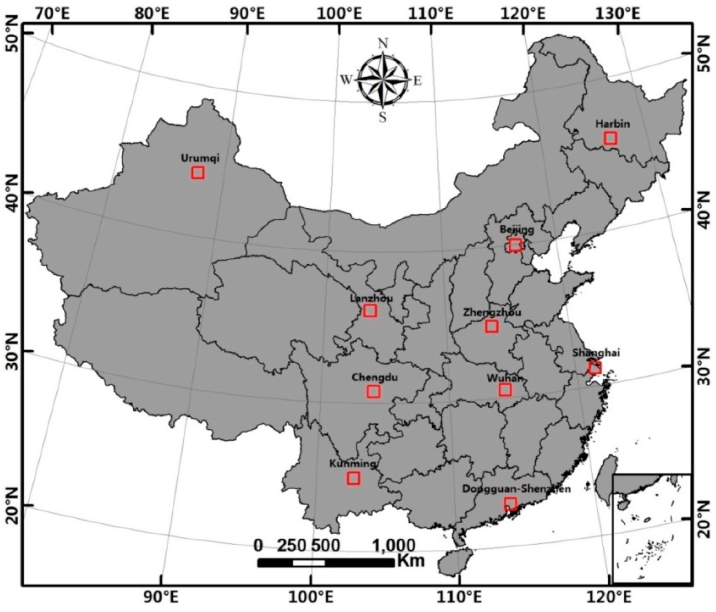
China has experienced unprecedented urbanization rates since the early 1980s due to the rural-to-urban population migration and economic conditions [2,3,45,46]. The urbanization patterns and rates vary greatly from coastal regions to central and western parts of the country and from southeastern to northeastern parts [45,46,47]. In order to develop ISA reference data for use in ISA modeling, ten metropolitan areas in different geographic locations and climate zones were selected (Figure 1). They have various population sizes, economic conditions, and administrative areas as summarized in Table 1. The complex landscapes, economic conditions, and topographic conditions in China provide an ideal example to explore approaches to rapidly map ISA spatial distribution and dynamic change.

Figure 1.
The study area—China and selected ten cities in red squares.

Table 1.
A summary of population, gross domestic product (GDP), and administrative area for the selected ten cities in 2012.
Different data sets as summarized in Table 2 were used in this research. The DMSP-OLS nighttime light data products (Version 4) with 6-bit data range and cell size of 1 × 1 km have the capability to acquire city lights, even low intensity from small residences and traffic lights, while sunlight, moonlight, glare, clouds, fires, and lighting features from auroras were removed through one-year data [30,48]. The MODIS NDVI 16-day composite (MOD13Q1) was generated from the daily MODIS Level-2G (L2G) surface reflectance. The constrained view angle-maximum value composite (CV-MVC) method was used to minimize the cloud contamination. The maximum NDVI value with the smallest view angle or the closest-to-nadir view for each pixel per 16-day composite interval was generated using MODIS Vegetation Indices (MOD13). The water mask product (MOD44W) with the cell size of 250 m × 250 m utilizes the SWBD (SRTM Water Body Data) and complements it with information from 250 m MODIS data to create a complete representation of global surface water (see detailed description in [49]). Landsat 8 Operational Land Imager (OLI) reflective bands were used to map ISA distribution for the selected sites.
Table 2.
Datasets used in research.
3. Methods
Figure 2 illustrates the framework of mapping fractional ISA distribution using the combination of DMSP-OLS, MODIS NDVI, and a limited number of Landsat 8 OLI data. The major steps include: (1) developing ISA data from Landsat 8 OLI data for the typical sites and aggregating the pixel ISA data at cell size of 25 m × 25 m to fractional ISA data at cell size of 250 m × 250 m; (2) preprocessing data for coarse spatial resolution images and implementing data integration using the indices; (3) developing ISA estimation models based on different indices using SVR; and (4) comparing and evaluating ISA estimation results.
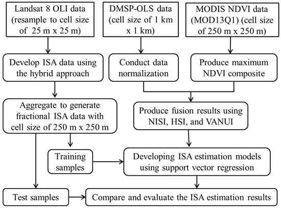
Figure 2.
Framework of mapping fractional ISA distribution through combination of multisource remote sensing data (ISA—impervious surface area; NISI—Normalized Impervious Surface Index; HSI—Human Settlement Index; VANUI—Vegetation Adjusted Nighttime light Urban Index; NDVI—Normalized Difference Vegetation Index).
3.1. Development of Impervious Surface Area Data from Landsat OLI Images
The Landsat 8 OLI data were re-projected from the Universal Transverse Mercator coordinate system to Albers Conical Equal Area projection, and the nearest-neighbor algorithm was used to resample the Landsat 8 OLI imagery with 30 m spatial resolution into a pixel size of 25 m × 25 m. A combination of thresholding and cluster analysis was used to extract ISA data from Landsat imagery [44]. We first produced NDVI and normalized difference water index (NDWI) to extract vegetation and water bodies. Based on analysis of vegetation and water sample plots, we selected a threshold of 0.3 in NDVI data to extract vegetation pixels (i.e., if a pixel has NDVI value of greater than 0.3, the pixel was assigned as vegetation) and a threshold of 0.1 in NDWI to extract water pixels (i.e., if a pixel has NDWI value of greater than 0.1, the pixel was assigned as water). After masking vegetation and water, the remaining pixels were mainly ISA and bare soils. Their spectral signatures were then extracted from the OLI imagery, and cluster analysis was conducted to classify the remaining pixels into 100 clusters. The analyst merged the clusters into ISA and others based on analysis of their spectral signatures. The ISA imagery was visually examined by overlaying it on the Landsat 8 OLI color composite to make sure the ISA pixels were properly extracted with high accuracy. Finally, the ISA imagery was aggregated from a cell size of 25 m × 25 m to a cell size of 250 m × 250 m to generate fractional ISA imagery based on the calculation of mean value within the window size of 10 by 10 pixels.
3.2. Preprocessing and Integration of DMSP-OLS and MODIS NDVI Data
Both DMSP-OLS and MODIS NDVI datasets were re-projected into Albers Conical Equal Area coordinate system. The nearest-neighbor resampling algorithm was used to resample the DMSP-OLS data to a cell size of 1 km × 1 km and resample the time-series MODIS NDVI data to a cell size of 250 m × 250 m. The DMSP-OLS data were normalized using Equation (1):
where is the normalized DMSP-OLS image. and represent the minimum and maximum values in the DMSP-OLS imagery, here they are 0 and 63.
The cloud and shadow contamination problem is common in the time-series MODIS NDVI data, especially in subtropical and tropical regions. In order to eliminate this problem and to reduce the confusion of bare soils in agricultural lands and ISA, a maximum algorithm using Equation (2) was used to produce a new composite:
where , , …, are the MOD13Q1 NDVI time series images. The global water data (MOD44W) were used to mask out water bodies from both and datasets, thus they have a data range between 0 and 1.
In DMSP-OLS data, coarse spatial resolution and small data range (0–63) result in data saturation and blooming effects [29,48], while the relatively high spatial resolution and high radiometric resolution in MODIS data make it possible to better distinguish different land cover types [29,36,37]. Because of the sensitivity of red and near-infrared wavelengths in separation of vegetation and non-vegetation types (e.g., ISA and water), NDVI has almost no data saturation problems in urban landscapes [29]. The different characteristics of DMSP-OLS and MODIS NDVI data result in the integrated use of both data sets, and this integration has been proven to produce better ISA extraction performance than using individual data alone [29,39,40,41]. It is critical to take advantage of both data sources in reducing data saturation problems in urban landscapes and reducing the blooming effects in suburban regions.
The common indices used in previous research are HSI [29,43] and VANUI [40], but they cannot effectively extract ISA when the proportion of ISA in a pixel is very small (e.g., less than 0.2) or very high (e.g., greater than 0.8). Here, we propose a new index called Normalized Impervious Surface Index (NISI) (Equation (3)) based on OLSnor (1 km × 1 km) and NDVImax (250 m × 250 m) for improving ISA mapping performance:
Here, we used NDVImax instead of NDVImean to eliminate cloud and shadow problems in tropical and subtropical regions and reduce the impacts of bare soils on the extraction of ISA. The inclusion of is to enhance the separation of vegetation and non-vegetation types in the urban landscapes when vegetation covers account for a small portion in a unit. The use of 0.5 before OLSnor is to reduce the influence of OLSnor values, and the use of 2 is to make sure the NISI values fall within the range of 0 and 1. is to enhance the difference between vegetation and non-vegetation, and is to enhance the difference of nighttime light values within the urban landscape. Therefore, NISI is to enlarge the difference between ISA and other land covers for better separation of ISA from other land covers in the complex urban landscape. The proposed index was compared to OLSnor and NDVImax using a typical line going through the urban landscape to examine the effectiveness of the new index in reducing data saturation and the blooming effects. In addition to the proposed NISI, another two indices—HSI and VANUI—were also calculated [29,40].
3.3. Mapping Fractional Impervious Surface Area Distribution with Support Vector Regression
The support vector machine is a supervised nonparametric statistical learning technique and has attracted great attention in recent decades due to its good performance in remote sensing–based classification [14,42,50,51]. Support vector machine is an integrated software package for supporting category classification and regression estimation. In this research, we used the support vector regression (SVR) to map fractional ISA distribution. The Gaussian radial basis function (RBF) kernel was used in the SVR modeling. There are three major steps: (1) input the reference samples from Landsat OLI and corresponding samples from the NISI imagery; (2) use the RBF kernel of the SVR modeling and optimize parameters through a cross-validation method; and (3) input NISI imagery and map fractional ISA distribution based on the optimized parameters. The same procedure is also used for ISA prediction using HSI and VANUI imagery.
A random sampling technique was used to collect samples from the fractional ISA imagery, NISI, HSI and VANUI images for each selected city. The fractional ISA data from the Landsat 8 OLI images were used as a dependent variable and the individual index (e.g., NISI, HSI and VANUI) was used separately as an independent variable to establish the relationship between fractional ISA reference data and NISI, HSI and VANUI, respectively, using the SVR approach. A total of 1500 ISA samples were extracted from ten reference images with 150 samples for each, as well as from the NISI, HSI and VANUI images. Of these samples, 1000 samples were randomly selected for modeling, and the remaining 500 samples were used for evaluation of ISA estimates. The optimized SVR model was used to predict ISA distribution for the entire study area.
3.4. Evaluation of the Impervious Surface Area Estimation Results
Accuracy assessment is often conducted at pixel level using the error matrix approach [52], but this approach is not suitable for evaluation of fractional ISA estimates in this research. Therefore, correlation coefficient (R), root mean squared error (RMSE), relative RMSE (RMSEr), and residual analysis were used to assess the fitness between the ISA estimates and reference data [29,44]. Meanwhile, the accuracy assessment was conducted at different ISA groups (e.g., <0.2, [0.2–0.4), [0.4–0.6), [0.6–0.8), and ≥0.8) to understand potential under/overestimation. In addition to the traditional approaches using R and RMSE for accuracy assessment, we also examined the accuracy of spatial prediction of fractional ISA maps by calculating means () using Equation (4) [53], where and represent the predicted ISA and reference data, and N and n represent the number of total predicted samples and reference samples:
4. Results
4.1. A Comparative Analysis of the Proposed Index and Individual OLSnor and NDVImax Data
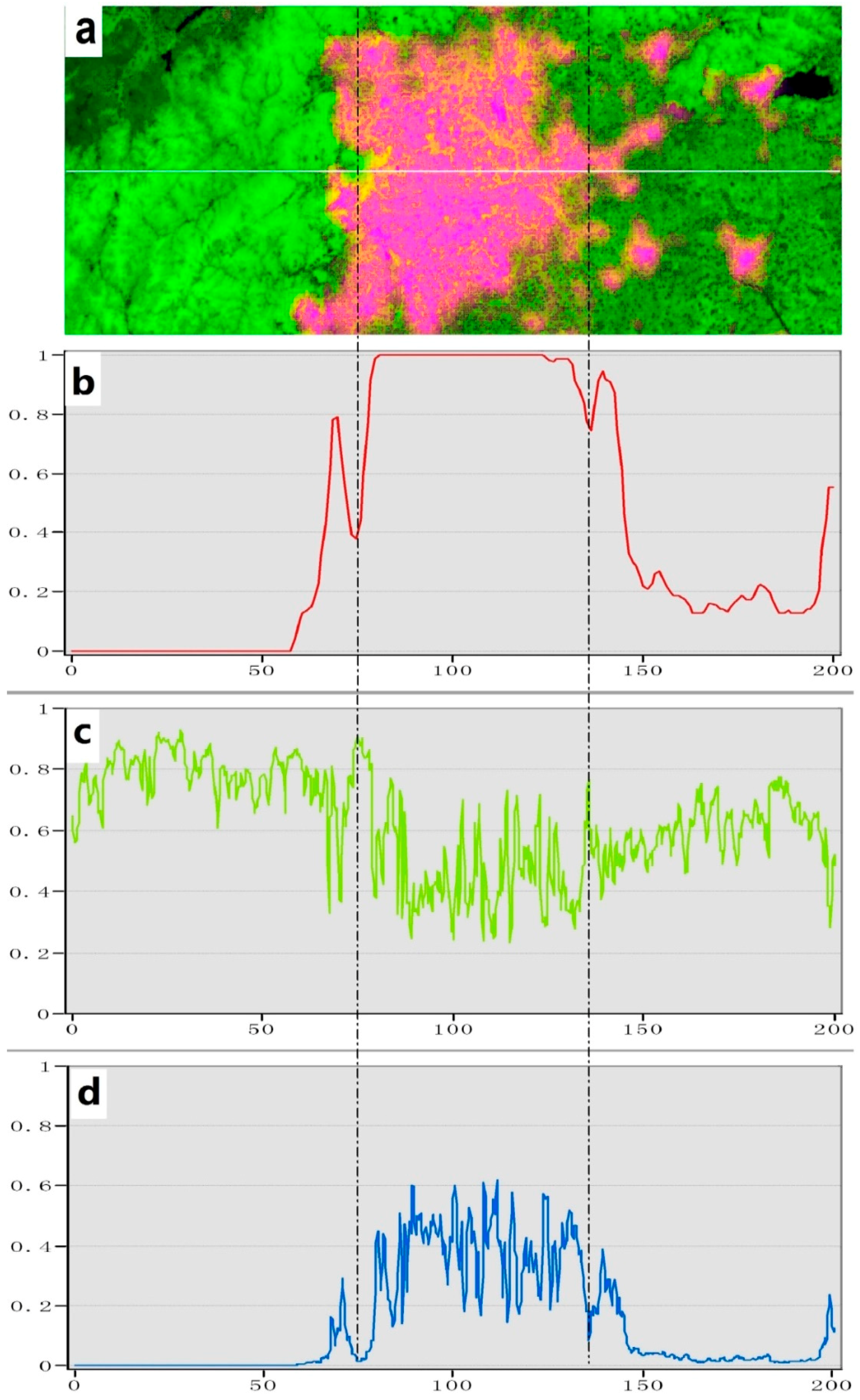
The effectiveness of the NISI data comparing with individual OLSnor and NDVImax data alone is illustrated in Figure 3. It indicates that the data-saturation problem in urban regions and blooming effects in the urban-rural interfaces are obvious in OLSnor data (Figure 3a,b), but not for NDVImax and NISI (Figure 3c,d). The NDVImax values vary, depending on the composition of vegetation and ISA in the urban landscape. The high spatial resolution in NDVImax data reduced the blooming effects (Figure 3c), and NISI provided much detailed information compared to OLSnor data alone, especially in the urban regions (Figure 3d). This implies that NISI has much more abundant information about urban land cover structures than OLSnor, thus the spatial patterns of ISA distribution may be much improved when NISI is used for ISA estimation.

Figure 3.
A false color composite based on (a) OLSnor, NDVImax, and NISI as red, green, and blue; and corresponding digital values of (b) OLSnor, (c) NDVImax, and (d) NISI based on the line in the urban landscape of Beijing. (Note: OLSnor is the normalized DMSP-OLS image, and NDVImax is a composite of NDVI time series data using the maximum algorithm).
4.2. Analysis of Impervious Surface Area Estimates
The accuracy assessment results in Table 3 indicate that the newly proposed NISI has slightly better performance than previously used two indices (i.e., HSI and VANUI). Overall, the NISI-based ISA prediction has the highest R and lowest RMSE and RMSEr values, followed by the VANUI-based predictions. HSI has relatively poor performance.
Table 3.
Accuracy assessment results from Human Settlement Index (HSI), Vegetation Adjusted Nighttime light Urban Index (VANUI), and Normalized Impervious Surface Index (NISI) using Support Vector Regression (SVR).
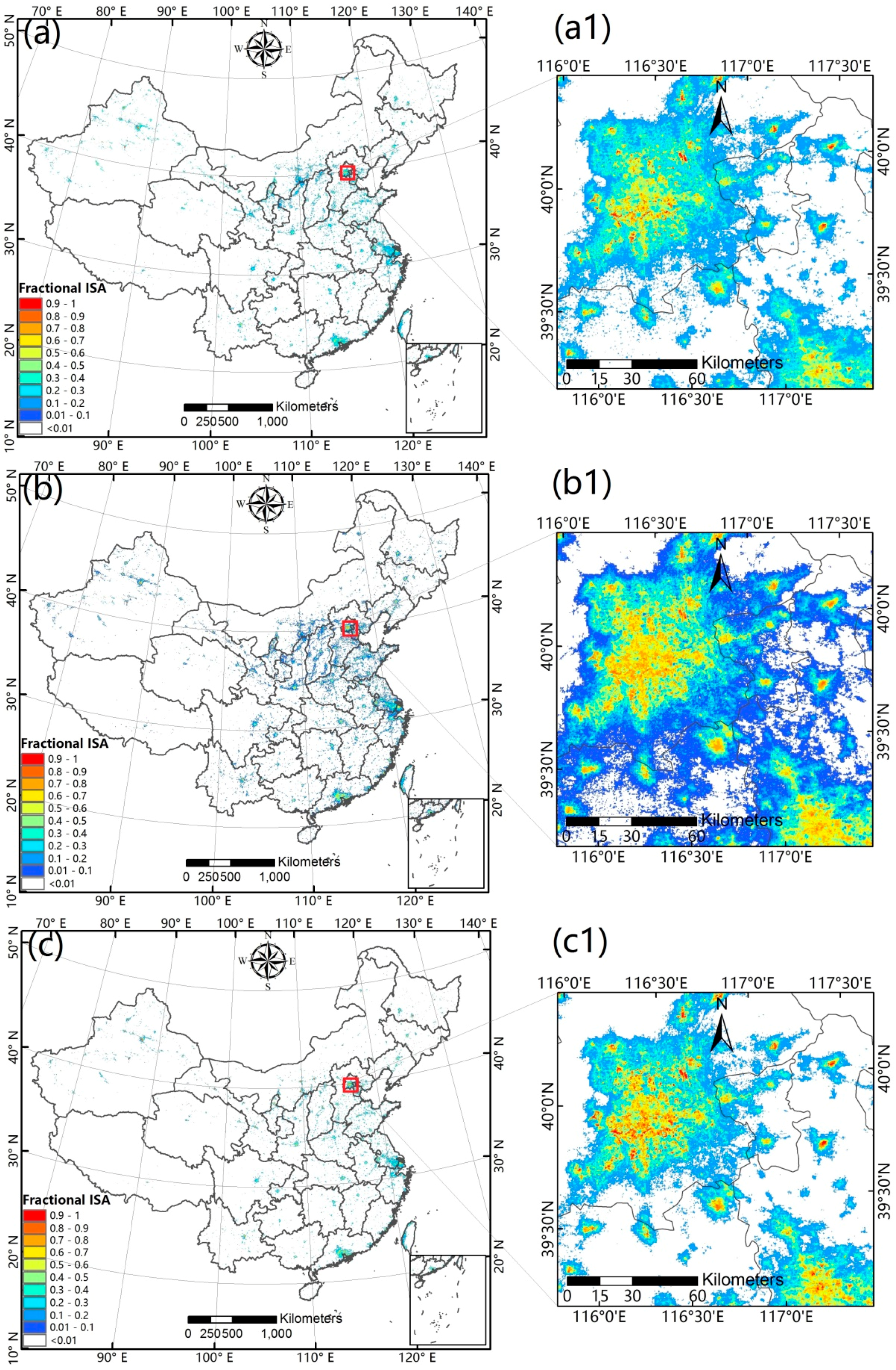
The spatial patterns of ISA distributions using these indices are illustrated in Figure 4. It indicates that the VANUI-derived ISA distribution (Figure 4b) has obviously the highest number of ISA pixels, followed by the HSI- (Figure 4a) and NISI-derived ISA results (Figure 4c)). Considering one city, for example, the VANUI-derived ISA distribution in Beijing (Figure 4(b1)) has the highest number of yellow pixels (ISA in 0.5–0.7), and NISI-derived results have the highest number of red pixels (Figure 4(c1), ISA > 0.8), and HSI-derived results have the lowest red and yellow pixels (Figure 4(a1), ISA > 0.5). In contrast, the VANUI-derived results have the highest number of blue pixels (i.e., ISA < 0.2), followed by the HSI-derived results, while the NISI-derived results have the least. This may imply that the NISI can better reduce the data saturation problem in the urban landscape, especially when ISA accounts for high proportions in a unit, and VANUI may have higher chances to overestimate ISA distribution than NISI when ISA is very small.
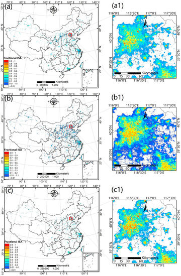
Figure 4.
Predicted impervious surface area distributions with the support vector regression method based on (a) HSI, (b) VANUI, and (c) NISI. Here (a1), (b1), and (c1) represent a typical location of impervious surface distribution corresponding to a, b, and c index respectively.
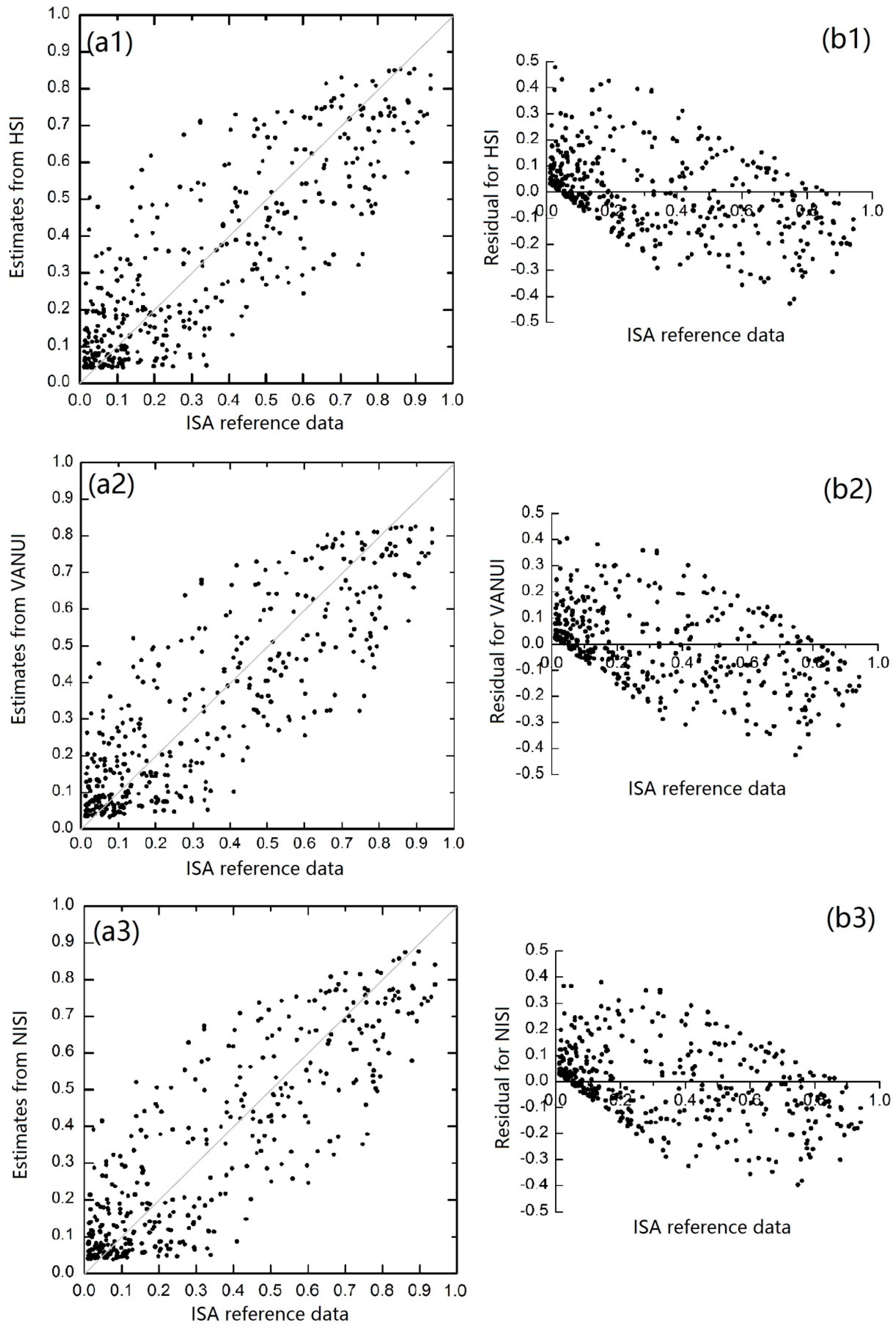
The scatterplots between estimates and reference data and residual analysis results (see Figure 5) can be better used to explain the prediction performance. It is obvious that when ISA is high (i.e., greater than 0.8), the NISI (Figure 5(a3)) has better performance in ISA prediction than HSI (Figure 5(a1)) and VANUI (Figure 5(a2)). The residual distributions indicate that when ISA is small (e.g., less than 0.4), NISI and VANUI have similar performance (Figure 5(b2,b3)) and have better performance than HSI (Figure 5(b1)). For the three indices, the majority of the test samples have residual values within the range of −0.3 and 0.3. However, Figure 5(b1,b2,b3) also shows clearly the underestimation and overestimation problems. For example, when ISA is greater than 0.8, ISA pixels are commonly underestimated; and when ISA is less than 0.1, the ISA pixels are overestimated.
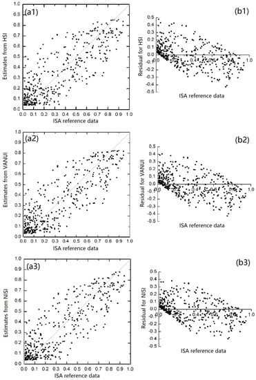
Figure 5.
The relationships between ISA estimates and reference data from different data sources and corresponding residual analysis results based on HSI (a1,b1), VANUI (a2,b2), and NISI (a3,b3).
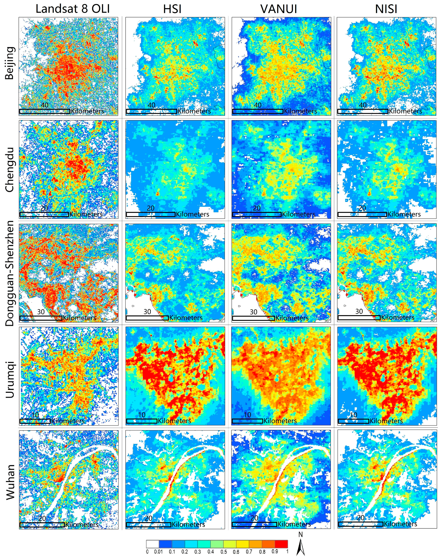
The under- or overestimation problems vary, depending on various cities, as shown in Figure 6. Overall, the ISA distribution using three indices for different cities present clear spatial patterns from the highest values in core urban areas to the lowest values in rural areas. However, the ISA estimation performances using the three indices are different; for example, NISI predicted the highest number of pixels with red (ISA > 0.9), VANUI predicted the highest number of pixels with yellow (ISA in 0.5–0.7) and blue (ISA < 0.1), while HSI predicted the highest number of pixels with cyan (ISA in 0.2–0.4) in these cities. All three indices overestimated ISA in Urumqi, and underestimated in Chengdu and Beijing, in comparison with the Landsat-derived ISA distribution. This situation may imply that ISA estimates using three indices have different uncertainties within the large area due to the unbalanced economic conditions and different climate conditions.
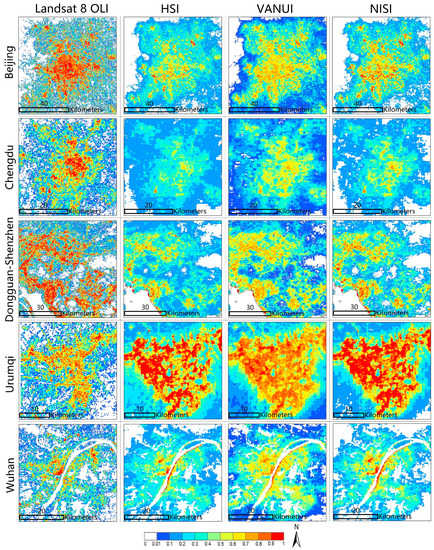
Figure 6.
A comparison of estimated ISA among different cities based on four data sources.
Table 4 indicates that, overall, the mean values from three indices are similar, and slightly less than the mean value from samples. However, when ISA is less than 0.4, these three mean values are higher than that from samples, implying that the three indices overestimate the ISA; in contrast, when ISA is greater than 0.4, mean values from the indices are smaller than that from samples, implying their underestimation. In particular, when ISA is greater than 0.8, the mean values from three indices are much lower than the mean from sample plots. Table 4 also indicates that the NISI-derived ISA data have mean values closer to the mean from samples than the HSI- and VANUI-derived predictions, implying that the NISI approach has better performance than the other two indices.
Table 4.
Evaluation of map applications by estimating the map means of fractional impervious surface area distributions.
In order to further examine the ISA prediction performance among the three indices, Table 5 summarizes RMSE and RMSEr results based on five ISA groups: <0.2, [0.2–0.4), [0.4–0.6), [0.6–0.8), and ≥0.8. Overall, the RMSEr declined as ISA proportion in a pixel increased no matter which index was used. These results also indicate that a NISI-based approach has less RMSEr values than HSI and VANUI when ISA is greater than 0.6 or less than 0.2, implying that the newly proposed index has better performance when ISA is very small or high. When ISA is in medium range in a pixel (i.e., 0.4–0.6), the three indices have similar performance. When ISA is in the range of 0.2 and 0.4, NISI has slightly poor performance than HSI and VANUI.
Table 5.
Comparison of root mean squared error (RMSE) and relative RMSE (RMSEr) results among three variables based on impervious surface area (ISA) ranges.
5. Discussion
DMSP-OLS data have been widely used for ISA mapping at regional and global scales [24,54]. However, the problems in mixed pixels (1 km spatial resolution), data saturation (0–63 data range), blooming effects, and the impacts of different socioeconomic conditions on DMSP-OLS radiances [29,30,40,41] have been recognized as major factors resulting in poor performance in extracting ISA distribution. Therefore, much research has explored the approaches to reduce these problems. One solution is to combine MODIS and DMSP-OLS data to produce a new product with improved spatial resolution and data ranges by taking the advantages of MODIS data in spatial resolution (250 m), radiometric resolution (12 bits), and good separation capacity in vegetation and non-vegetation (e.g., ISA, water) types. For example, previous research has proposed HSI [29], VANUI [40] and EANTLI [41] to reduce the data saturation problem, and has been proven effective in improving ISA estimation accuracy and spatial patterns. This research further confirmed the necessity of integrating DMSP-OLS and MODIS data in improving ISA mapping performance, and the newly developed NISI can further improve ISA mapping performance. This research indicates that the newly proposed NISI has better capability in ISA mapping than HSI and VANUI when ISA is very small (ISA is less than 0.2) and high (ISA is higher than 0.6). VANUI has the potential to overestimate ISA pixels with small values. This is because the mean values used in NDVI time series data sets cannot eliminate the impacts of clouds and bare soils, while the maximum values of NDVI time series data sets can solve this problem. Another advantage of using NISI is its capability in further improving the spatial structure in urban landscapes, thus NISI has better ISA prediction performance than HSI and VANUI when ISA is high. As global Landsat data are available, the integration of DMSP-OLS and Landsat NDVI will be another choice for improving ISA mapping [55]. The advance of computing (e.g., Google Earth Engine, Google Cloud) and satellite technologies will make the effective use of multi-source data an important research topic in improving ISA mapping performance at regional and global scales [18].
The ISA estimation uncertainty varies in different cities (see Figure 6). Some cities in arid/semiarid regions such as Urumqi mainly suffered from an overestimation problem, while Dongguan-Shenzhen in south China and Chengdu in west China appeared to suffer from an underestimation problem. In addition to the economic conditions that directly affect DMSP-OLS radiance values, climate condition may be another factor indirectly affecting DMSP-OLS radiances. Previous research has shown that vegetation indices or abundance has highly negative correlation with ISA in urban landscapes, thus ISA can be estimated from the vegetation index [11]. However, this relationship in arid and semiarid regions becomes poor because of limited vegetation covers in and around urban regions. In this situation, integration of vegetation indices and DMSP-OLS data cannot reduce the blooming effects and data saturation problems. To date, there is little research to explore the potential to accurately extract ISA in arid/semiarid regions. One solution may be use of temperature during the winter season when buildings in winter have higher temperature than surrounding bare soils due to human activities in urban areas. Use of MODIS temperature products may be valuable, but their coarse spatial resolution is problematic. An alternative is to use Landsat thermal bands [20]. More research is needed to explore the incorporation of temperature data into DMSP-OLS or/and MODIS data to improve ISA mapping performance. ISA modeling based on different climate zones and/or economic conditions may be needed in the future for further improving estimation accuracy.
6. Conclusions
Regional and global ISA mapping has attracted much attention in the past two decades due to its importance in different applications such as urban environmental change, population and economic studies, and climate change. This research proposes a new index called NISI and compares it to previously used indices—HSI and VANUI—in ISA estimation in China using the SVR approach. This research has proven the promise of accurately mapping ISA distribution in a large area. Comparing with the two previously used indices, HSI and VANUI, the newly developed index can further improve ISA mapping performance, especially when the ISA proportion in a pixel is very small (e.g., <0.2) and relatively high (e.g., >0.6). This research confirmed the necessity to integrate DMSP-OLS and MODIS NDVI data to improve ISA estimation. More research should be explored to improve ISA estimation in arid and semiarid regions.
Acknowledgments
The study was financially supported by the Zhejiang Agriculture and Forestry University’s Research and Development Fund (2013FR052). We also thank the Center for Global Change and Earth Observations at Michigan State University for providing the facility support.
Author Contributions
Dengsheng Lu and Wenhui Kuang conceived and designed the experiments; Wei Guo performed the experiments and analyzed the data; Dengsheng Lu wrote the paper; and all authors edited the paper.
Conflicts of Interest
The authors declare no conflict of interest. The founding sponsors had no role in the design of the study; in the collection, analyses, or interpretation of data; in the writing of the manuscript, and in the decision to publish the results.
References
- Cao, X.; Wang, J.; Chen, J.; Shi, F. Spatialization of electricity consumption of China using saturation-corrected DMSP-OLS data. Int. J. Appl. Earth Obs. Geoinf. 2014, 28, 193–200. [Google Scholar] [CrossRef]
- Kuang, W.; Liu, J.; Zhang, Z.; Lu, D.; Xiang, B. Spatiotemporal dynamics of impervious surface areas across China during the early 21st century. Chin. Sci. Bull. 2012, 58, 1691–1701. [Google Scholar] [CrossRef]
- Schneider, A.; Chang, C.; Paulsen, K. The changing spatial form of cities in western China. Landsc. Urban Plan. 2015, 135, 40–61. [Google Scholar] [CrossRef]
- China–Population. Available online: http://countryeconomy.com/demography/population/china (accessed on 14 April 2017).
- Urbanization in China. Available online: https://en.wikipedia.org/wiki/Urbanization_in_China (accessed on 14 April 2017).
- Kaufmann, R.K.; Seto, K.C.; Schneider, A.; Liu, Z.; Zhou, L.; Wang, W. Climate response to rapid urban growth: Evidence of a human-induced precipitation deficit. J. Clim. 2007, 20, 2299–2306. [Google Scholar] [CrossRef]
- Ma, T.; Zhou, C.; Pei, T.; Haynie, S.; Fan, J. Quantitative estimation of urbanization dynamics using time series of DMSP/OLS nighttime light data: A comparative case study from China’s cities. Remote Sens. Environ. 2012, 124, 99–107. [Google Scholar] [CrossRef]
- Ma, T.; Zhou, Y.; Zhou, C.; Haynie, S.; Pei, T.; Xu, T. Night-time light derived estimation of spatiotemporal characteristics of urbanization dynamics using DMSP/OLS satellite data. Remote Sens. Environ. 2015, 158, 453–464. [Google Scholar] [CrossRef]
- Srinivasan, V.; Seto, K.C.; Emerson, R.; Gorelick, S.M. The impact of urbanization on water vulnerability: A coupled human–environment system approach for Chennai, India. Glob. Environ. Chang. 2013, 23, 229–239. [Google Scholar] [CrossRef]
- Xu, H.; Lin, D.; Tang, F. The impact of impervious surface development on land surface temperature in a subtropical city: Xiamen, China. Int. J. Climatol. 2013, 33, 1873–1883. [Google Scholar] [CrossRef]
- Yuan, F.; Bauer, M.E. Comparison of impervious surface area and normalized difference vegetation index as indicators of surface urban heat island effects in Landsat imagery. Remote Sens. Environ. 2007, 106, 375–386. [Google Scholar] [CrossRef]
- Kuang, W.; Chi, W.; Lu, D.; Dou, Y. A comparative analysis of megacity expansions in China and the U.S.: Patterns, rates and driving forces. Landsc. Urban Plan. 2014, 132, 121–135. [Google Scholar] [CrossRef]
- Mertes, C.M.; Schneider, A.; Sulla-Menashe, D.; Tatem, A.J.; Tan, B. Detecting change in urban areas at continental scales with MODIS data. Remote Sens. Environ. 2015, 158, 331–347. [Google Scholar] [CrossRef]
- Pandey, B.; Joshi, P.K.; Seto, K.C. Monitoring urbanization dynamics in India using DMSP/OLS night time lights and SPOT-VGT data. Int. J. Appl. Earth Obs. Geoinf. 2013, 23, 49–61. [Google Scholar] [CrossRef]
- Schneider, A. Monitoring land cover change in urban and peri-urban areas using dense time stacks of Landsat satellite data and a data mining approach. Remote Sens. Environ. 2012, 124, 689–704. [Google Scholar] [CrossRef]
- Zhang, Q.; Seto, K.C. Mapping urbanization dynamics at regional and global scales using multi-temporal DMSP/OLS nighttime light data. Remote Sens. Environ. 2011, 115, 2320–2329. [Google Scholar] [CrossRef]
- Zhou, Y.; Smith, S.J.; Zhao, K.; Imhoff, M.; Thomson, A.; Bond-Lamberty, B.; Asrar, G.R.; Zhang, X.; He, C.; Elvidge, C.D. A global map of urban extent from nightlights. Environ. Res. Lett. 2015, 10, 054011. [Google Scholar] [CrossRef]
- Lu, D.; Li, G.; Kuang, W.; Moran, E. Methods to extract impervious surface areas from satellite images. Int. J. Digit. Earth 2013, 7, 93–112. [Google Scholar] [CrossRef]
- Lu, D.; Li, G.; Moran, E.; Batistella, M.; Freitas, C.C. Mapping impervious surfaces with the integrated use of Landsat thematic mapper and radar data: A case study in an urban–rural landscape in the Brazilian Amazon. ISPRS J. Photogramm. Remote Sens. 2011, 66, 798–808. [Google Scholar] [CrossRef]
- Lu, D.; Weng, Q. Use of impervious surface in urban land-use classification. Remote Sens. Environ. 2006, 102, 146–160. [Google Scholar] [CrossRef]
- Weng, Q. Remote sensing of impervious surfaces in the urban areas: Requirements, methods, and trends. Remote Sens. Environ. 2012, 117, 34–49. [Google Scholar] [CrossRef]
- Wu, C.; Murray, A.T. Estimating impervious surface distribution by spectral mixture analysis. Remote Sens. Environ. 2003, 84, 493–505. [Google Scholar] [CrossRef]
- Elvidge, C.; Tuttle, B.; Sutton, P.; Baugh, K.; Howard, A.; Milesi, C.; Bhaduri, B.; Nemani, R. Global distribution and density of constructed impervious surfaces. Sensors 2007, 7, 1962–1979. [Google Scholar] [CrossRef]
- Ma, Q.; He, C.; Wu, J.; Liu, Z.; Zhang, Q.; Sun, Z. Quantifying spatiotemporal patterns of urban impervious surfaces in China: An improved assessment using nighttime light data. Landsc. Urban Plan. 2014, 130, 36–49. [Google Scholar] [CrossRef]
- Yang, Y.; He, C.; Zhang, Q.; Han, L.; Du, S. Timely and accurate national-scale mapping of urban land in China using defense meteorological satellite program’s operational Linescan system nighttime stable light data. APPRES 2013, 7, 073535. [Google Scholar] [CrossRef]
- Imhoff, M.L.; Lawrence, W.T.; Stutzer, D.C.; Elvidge, C.D. A technique for using composite DMSP/OLS “city lights” satellite data to map urban area. Remote Sens. Environ. 1997, 61, 361–370. [Google Scholar] [CrossRef]
- Henderson, M.; Yeh, E.T.; Gong, P.; Elvidge, C.; Baugh, K. Validation of urban boundaries derived from global night-time satellite imagery. Int. J. Remote Sens. 2003, 24, 595–609. [Google Scholar] [CrossRef]
- Lawrence, W.T.; Imhoff, M.L.; Kerle, N.; Stutzer, D. Quantifying urban land use and impact on soils in Egypt using diurnal satellite imagery of the earth surface. Int. J. Remote Sens. 2010, 23, 3921–3937. [Google Scholar] [CrossRef]
- Lu, D.; Tian, H.; Zhou, G.; Ge, H. Regional mapping of human settlements in southeastern china with multisensor remotely sensed data. Remote Sens. Environ. 2008, 112, 3668–3679. [Google Scholar] [CrossRef]
- Elvidge, C.D.; Baugh, K.E.; Dietz, J.B.; Bland, T.; Sutton, P.C.; Kroehl, H.W. Radiance calibration of DMSP-OLS low-light imaging data of human settlements. Remote Sens. Environ. 1999, 68, 77–88. [Google Scholar] [CrossRef]
- Ma, L.; Wu, J.; Li, W.; Peng, J.; Liu, H. Evaluating saturation correction methods for DMSP/OLS nighttime light data: A case study from China’s cities. Remote Sens. 2014, 6, 9853–9872. [Google Scholar] [CrossRef]
- Small, C.; Elvidge, C.D.; Balk, D.; Montgomery, M. Spatial scaling of stable night lights. Remote Sens. Environ. 2011, 115, 269–280. [Google Scholar] [CrossRef]
- Zhang, Q.; Seto, K. Can night-time light data identify typologies of urbanization? A global assessment of successes and failures. Remote Sens. 2013, 5, 3476–3494. [Google Scholar] [CrossRef]
- Deng, C.; Wu, C. The use of single-date MODIS imagery for estimating large-scale urban impervious surface fraction with spectral mixture analysis and machine learning techniques. ISPRS J. Photogramm. Remote Sens. 2013, 86, 100–110. [Google Scholar] [CrossRef]
- Knight, J.; Voth, M. Mapping impervious cover using multi-temporal MODIS NDVI data. IEEE J. Sel. Top. Appl. Earth Obs. Remote Sens. 2011, 4, 303–309. [Google Scholar] [CrossRef]
- Schneider, A.; Friedl, M.A.; Potere, D. A new map of global urban extent from MODIS satellite data. Environ. Res. Lett. 2009, 4, 044003. [Google Scholar] [CrossRef]
- Schneider, A.; Friedl, M.A.; Potere, D. Mapping global urban areas using MODIS 500-m data: New methods and datasets based on ‘urban ecoregions’. Remote Sens. Environ. 2010, 114, 1733–1746. [Google Scholar] [CrossRef]
- Yang, F.; Matsushita, B.; Fukushima, T.; Yang, W. Temporal mixture analysis for estimating impervious surface area from multi-temporal MODIS NDVI data in Japan. ISPRS J. Photogramm. Remote Sens. 2012, 72, 90–98. [Google Scholar] [CrossRef]
- Shao, Z.; Liu, C. The integrated use of DMSP/OLS nighttime light and MODIS data for monitoring large-scale impervious surface dynamics: A case study in the Yangtze River delta. Remote Sens. 2014, 6, 9359–9378. [Google Scholar] [CrossRef]
- Zhang, Q.; Schaaf, C.; Seto, K.C. The vegetation adjusted NTL urban index: A new approach to reduce saturation and increase variation in nighttime luminosity. Remote Sens. Environ. 2013, 129, 32–41. [Google Scholar] [CrossRef]
- Zhuo, L.; Zheng, J.; Zhang, X.; Li, J.; Liu, L. An improved method of night-time light saturation reduction based on EVI. Int. J. Remote Sens. 2015, 36, 4114–4130. [Google Scholar] [CrossRef]
- Cao, X.; Chen, J.; Imura, H.; Higashi, O. A SVM-based method to extract urban areas from DMSP-OLS and SPOT VGT data. Remote Sens. Environ. 2009, 113, 2205–2209. [Google Scholar] [CrossRef]
- Kuang, W. Evaluating impervious surface growth and its impacts on water environment in Beijing-Tianjin-Tangshan metropolitan area. J. Geogr. Sci. 2012, 22, 535–547. [Google Scholar] [CrossRef]
- Guo, W.; Lu, D.; Wu, Y.; Zhang, J. Mapping impervious surface distribution with integration of SNNP VIIRS DNB and MODIS NDVI data. Remote Sens. 2015, 7, 12459–12477. [Google Scholar] [CrossRef]
- Liu, J.; Zhang, Q.; Hu, Y. Regional differences of China’s urban expansion from late 20th to early 21st century based on remote sensing information. Chin. Geogr. Sci. 2012, 22, 1–14. [Google Scholar] [CrossRef]
- Schneider, A.; Mertes, C.M.; Tatem, A.J.; Tan, B.; Sulla-Menashe, D.; Graves, S.J.; Patel, N.N.; Horton, J.A.; Gaughan, A.E.; Rollo, J.T.; et al. A new urban landscape in east–southeast Asia, 2000–2010. Environ. Res. Lett. 2015, 10, 034002. [Google Scholar] [CrossRef]
- Sutton, P.C.; Elvidge, C.D.; Baugh, K.; Ziskin, D. Mapping the constructed surface area density for China. Proc. Asia-Pac. Adv. Netw. 2011, 31, 69. [Google Scholar] [CrossRef]
- Elvidge, C.D.; Imhoff, M.L.; Baugh, K.E.; Hobson, V.R.; Nelson, I.; Safran, J.; Dietz, J.B.; Tuttle, B.T. Night-time lights of the world: 1994–1995. ISPRS J. Photogramm. Remote Sens. 2001, 56, 81–99. [Google Scholar] [CrossRef]
- Carroll, M.L.; Townshend, J.R.; DiMiceli, C.M.; Noojipady, P.; Sohlberg, R.A. A new global raster water mask at 250 m resolution. Int. J. Digit. Earth 2009, 2, 291–308. [Google Scholar] [CrossRef]
- Brenning, A. Benchmarking classifiers to optimally integrate terrain analysis and multispectral remote sensing in automatic rock glacier detection. Remote Sens. Environ. 2009, 113, 239–247. [Google Scholar] [CrossRef]
- Mountrakis, G.; Im, J.; Ogole, C. Support vector machines in remote sensing: A review. ISPRS J. Photogramm. Remote Sens. 2011, 66, 247–259. [Google Scholar] [CrossRef]
- Congalton, R.G. A review of assessing the accuracy of classifications of remotely sensed data. Remote Sens. Environ. 1991, 37, 35–46. [Google Scholar] [CrossRef]
- McRoberts, R.E.; Næsset, E.; Gobakken, T. Inference for lidar-assisted estimation of forest growing stock volume. Remote Sens. Environ. 2013, 128, 268–275. [Google Scholar] [CrossRef]
- Elvidge, C.D.; Cinzano, P.; Pettit, D.R.; Arvesen, J.; Sutton, P.; Small, C.; Nemani, R.; Longcore, T.; Rich, C.; Safran, J.; et al. The Nightsat mission concept. Int. J. Remote Sens. 2007, 28, 2645–2670. [Google Scholar] [CrossRef]
- Zhang, Q.; Li, B.; Thau, D.; Moore, R. Building a better urban picture: Combining day and night remote sensing imagery. Remote Sens. 2015, 7, 11887–11913. [Google Scholar] [CrossRef]

© 2017 by the authors. Licensee MDPI, Basel, Switzerland. This article is an open access article distributed under the terms and conditions of the Creative Commons Attribution (CC BY) license (http://creativecommons.org/licenses/by/4.0/).