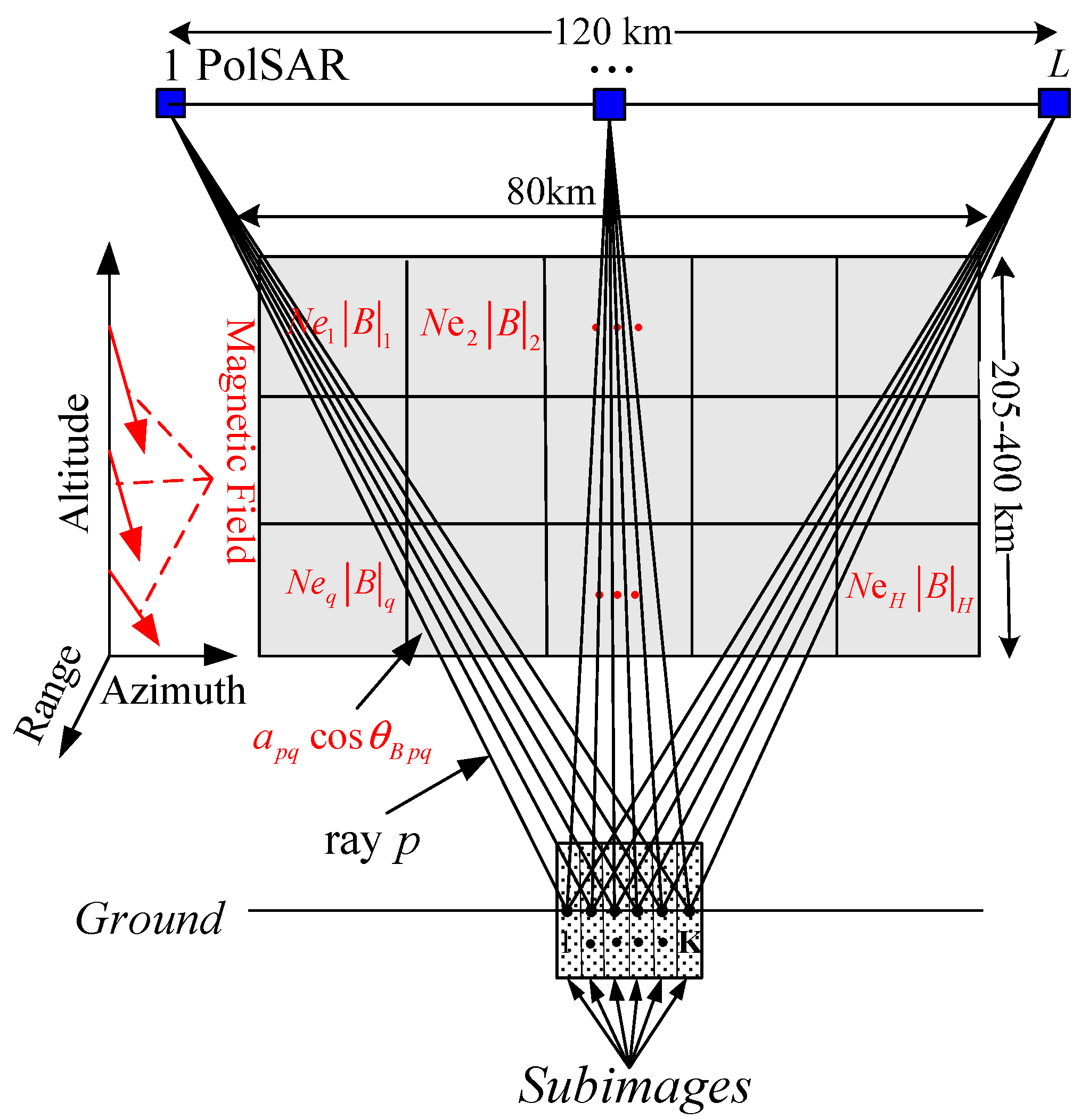
Figure 1.
Map of two-dimensional CIT using FR angles.
Figure 1.
Map of two-dimensional CIT using FR angles.
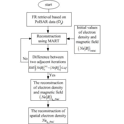
Figure 2.
The flowchart of the proposed CIT technique.
Figure 2.
The flowchart of the proposed CIT technique.
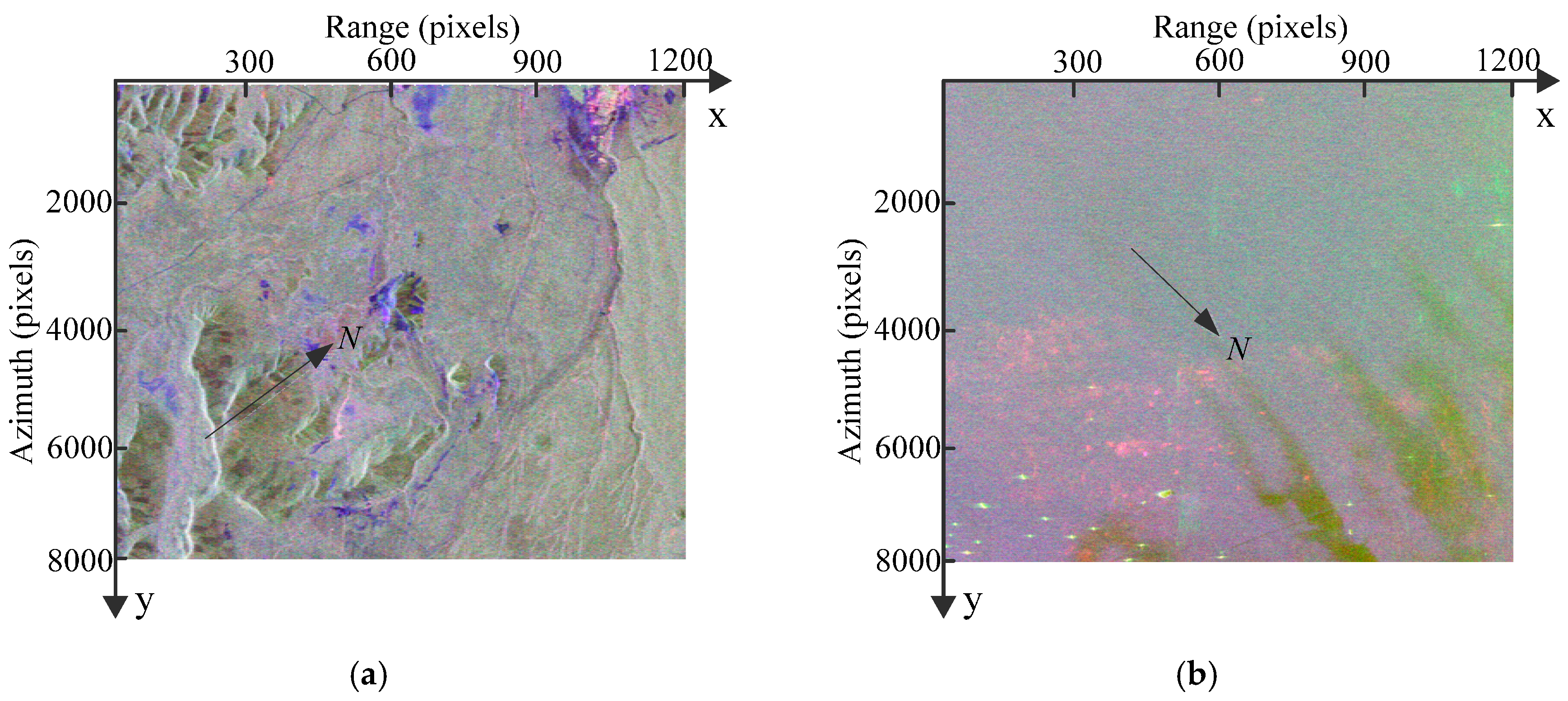
Figure 3.
The PALSAR polarimetric images in two areas. (a) Changbai Mountain (N, E) acquired on 3 December 2007 and (b) Qingdao (N, E) acquired on 29 March 2011.
Figure 3.
The PALSAR polarimetric images in two areas. (a) Changbai Mountain (N, E) acquired on 3 December 2007 and (b) Qingdao (N, E) acquired on 29 March 2011.
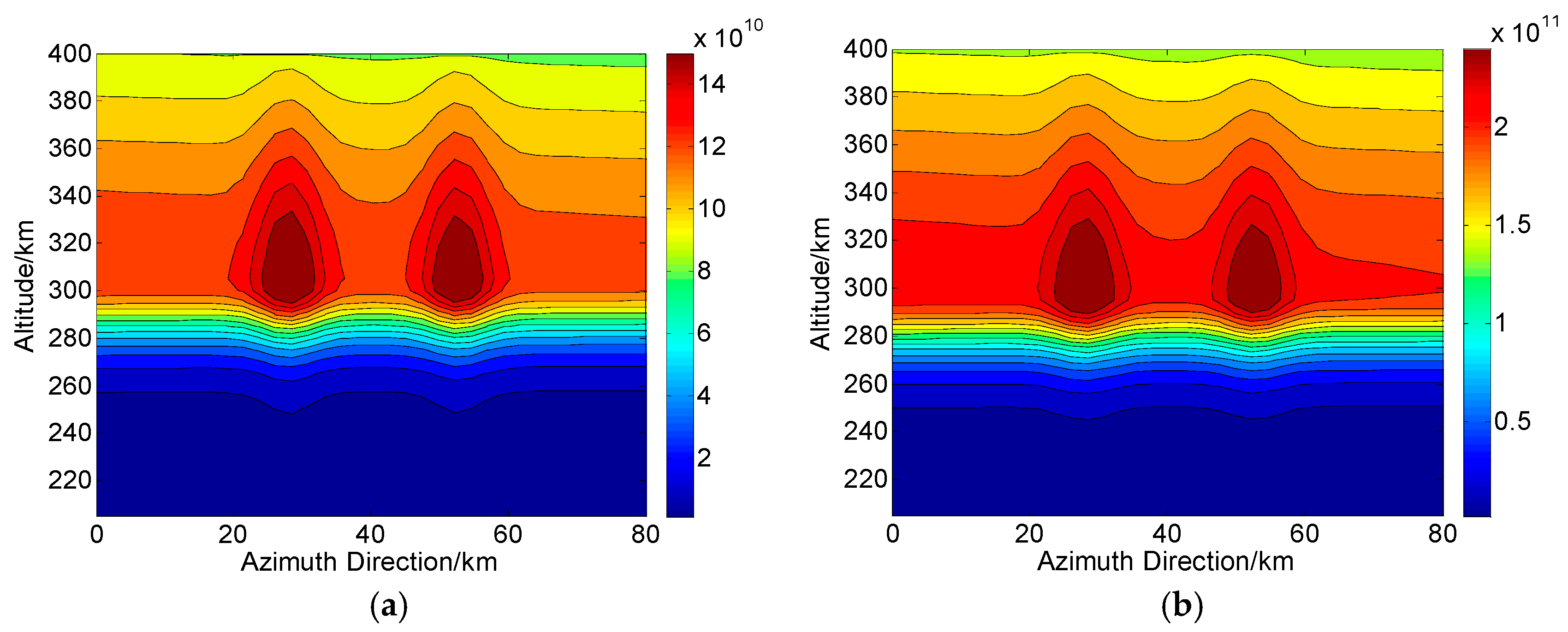
Figure 4.
The true distributions of electron density in areas of (a) Changbai and (b) Qingdao. The unit of the electron density is .
Figure 4.
The true distributions of electron density in areas of (a) Changbai and (b) Qingdao. The unit of the electron density is .
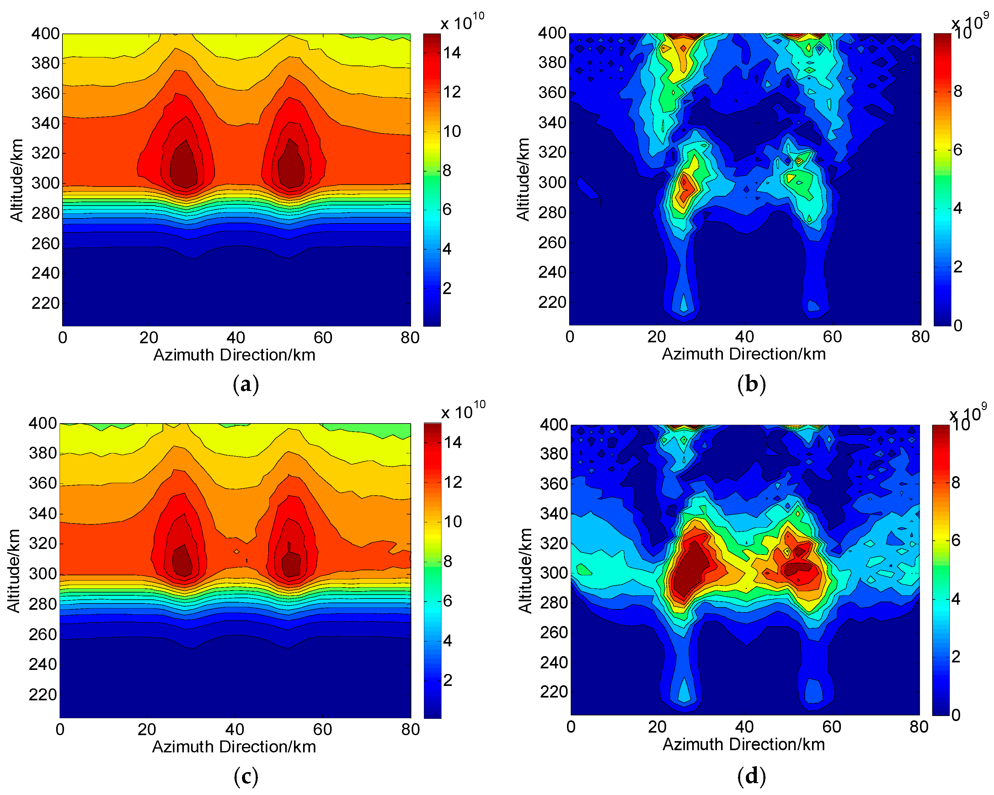
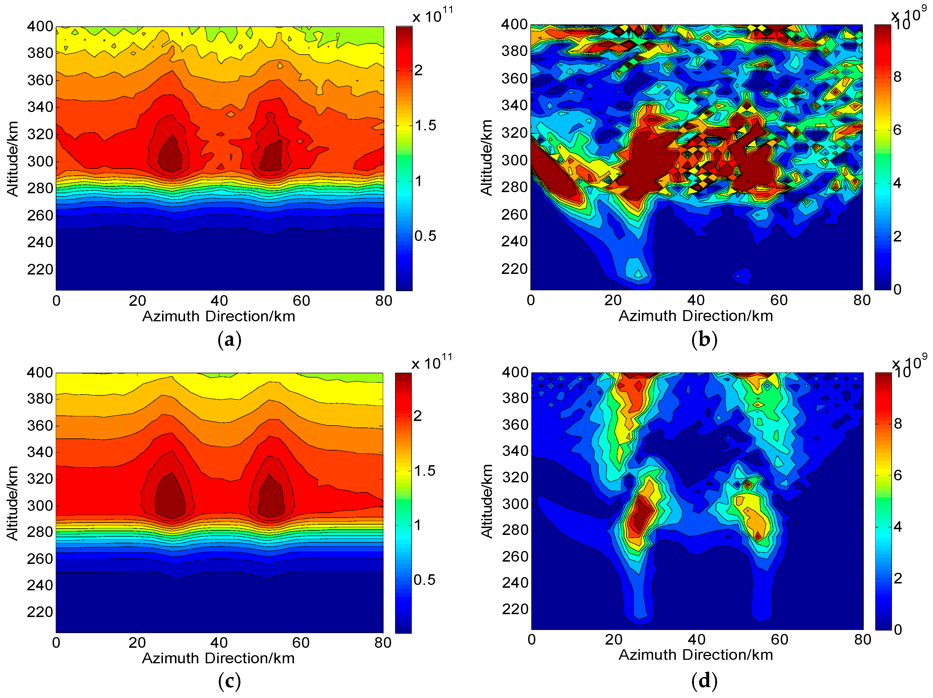
Figure 5.
Two-dimensional CIT reconstructions without system errors in Changbai. (a,c) are the reconstructed results based on proposed and traditional CIT methods, respectively. (b,d) are the corresponding absolute deviations between the true and reconstructed results. The unit of the electron density is .
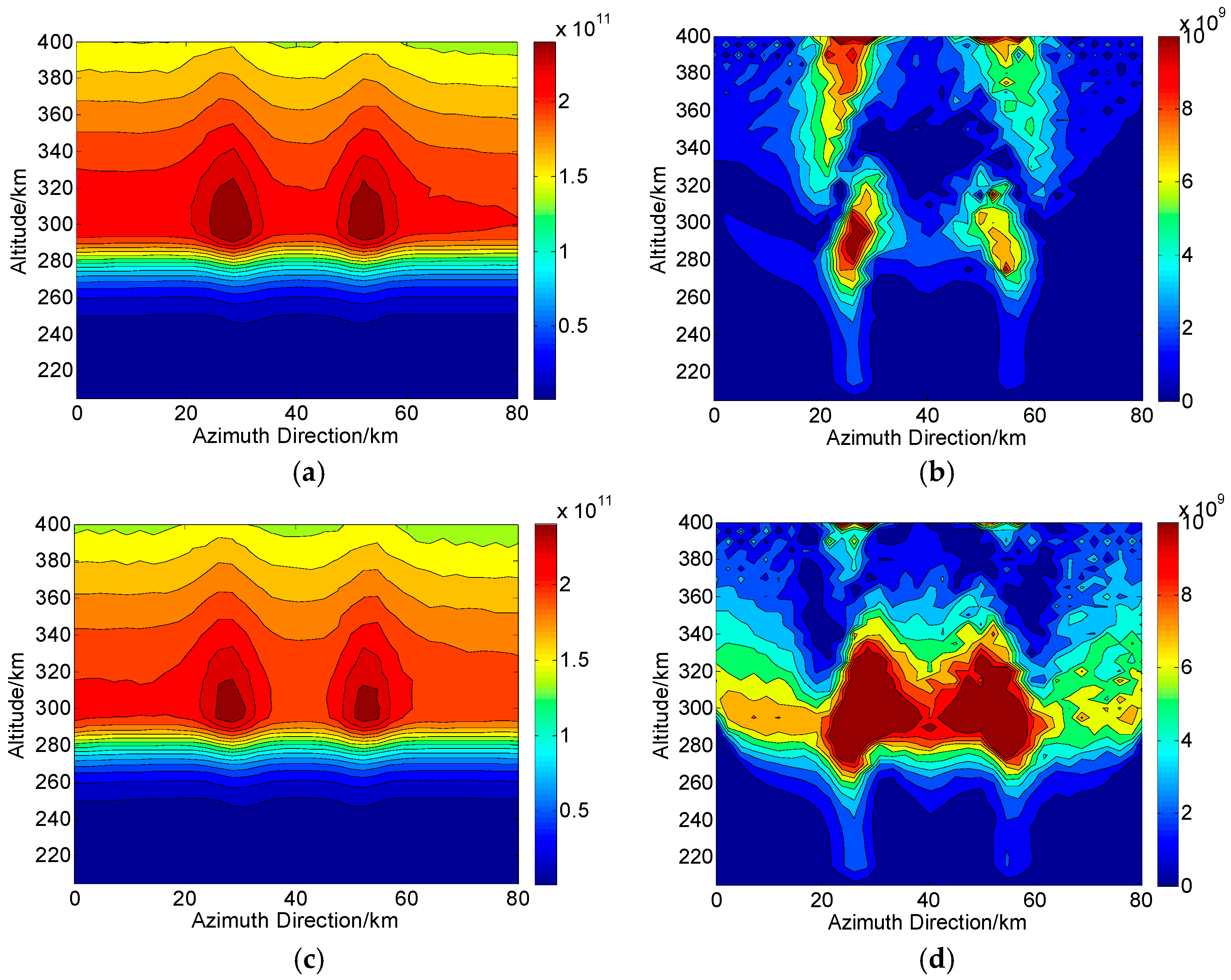
Figure 6.
Two-dimensional CIT reconstructions without system errors in Qingdao. (a,c) are the reconstructed results based on proposed and traditional CIT methods, respectively. (b,d) are the corresponding absolute deviations between the true and reconstructed results. The unit of the electron density is .
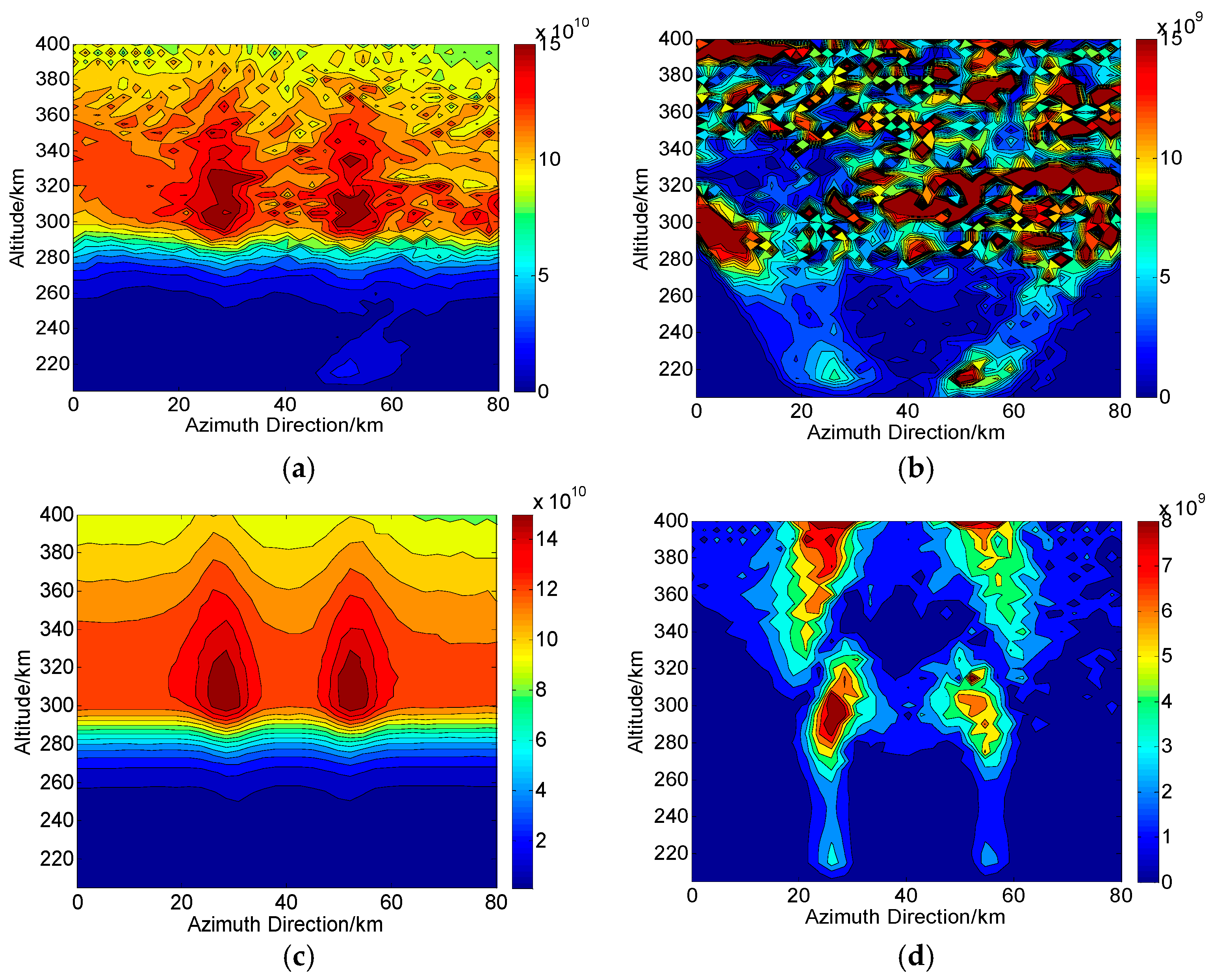
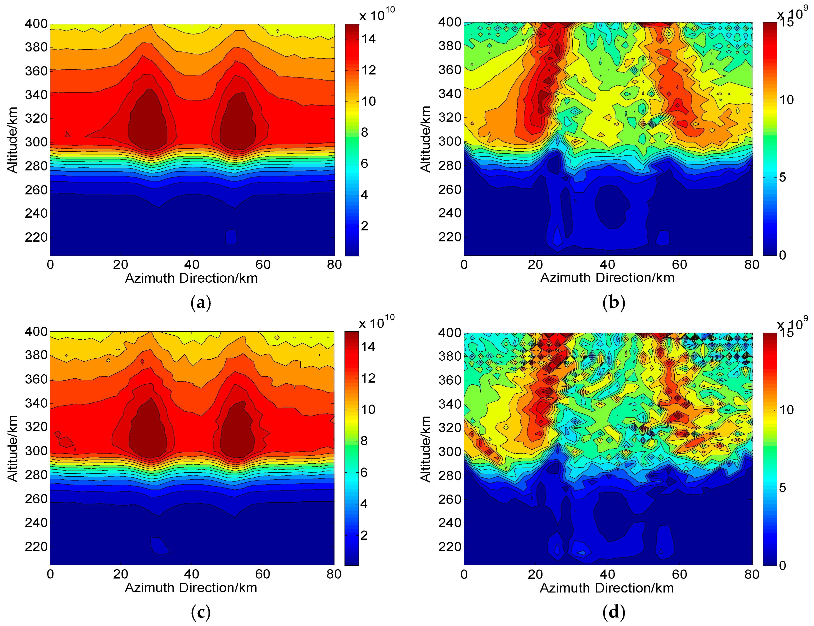
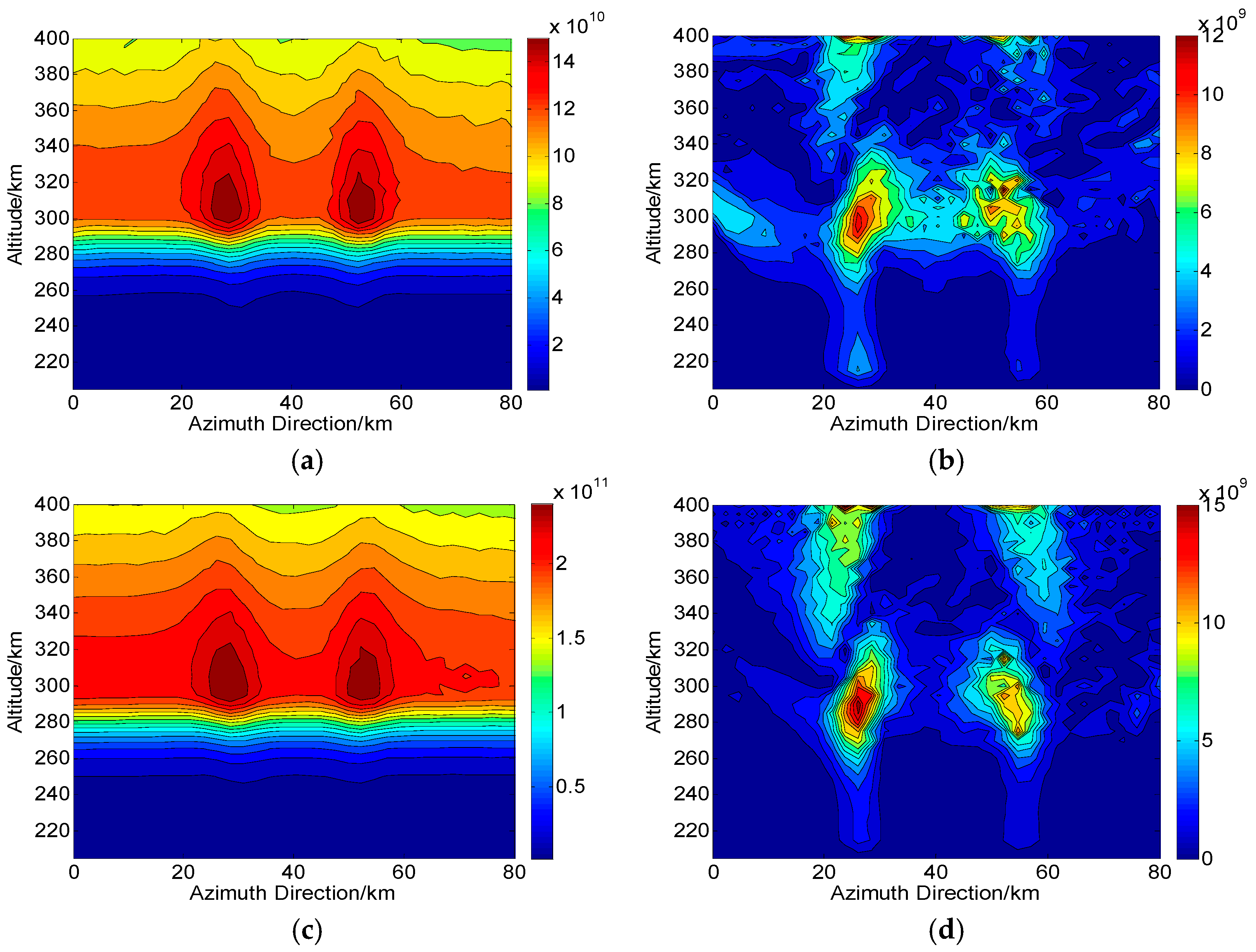
Figure 7.
Two-dimensional CIT reconstructions under the condition of system noise in Changbai ( is used). (a,c) are the reconstructed results with and , respectively. (b,d) are the corresponding absolute deviations between the true and reconstructed results. The unit of the electron density is .
Figure 7.
Two-dimensional CIT reconstructions under the condition of system noise in Changbai ( is used). (a,c) are the reconstructed results with and , respectively. (b,d) are the corresponding absolute deviations between the true and reconstructed results. The unit of the electron density is .
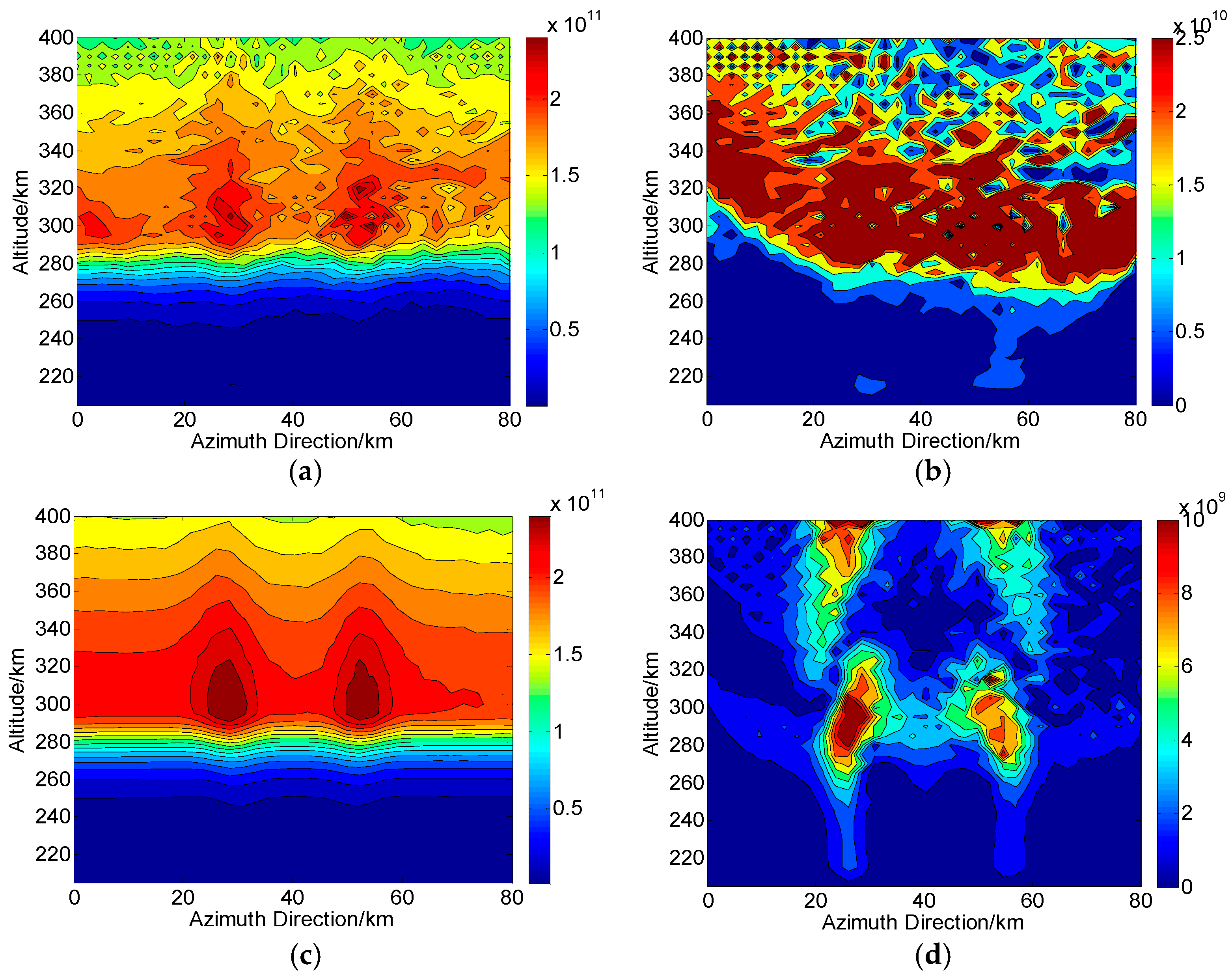
Figure 8.
Two-dimensional CIT reconstructions under the condition of system noise in Qingdao ( is used). (a,c) are the reconstructed results with and , respectively. (b,d) are the corresponding absolute deviations between the true and reconstructed results. The unit of the electron density is .
Figure 8.
Two-dimensional CIT reconstructions under the condition of system noise in Qingdao ( is used). (a,c) are the reconstructed results with and , respectively. (b,d) are the corresponding absolute deviations between the true and reconstructed results. The unit of the electron density is .
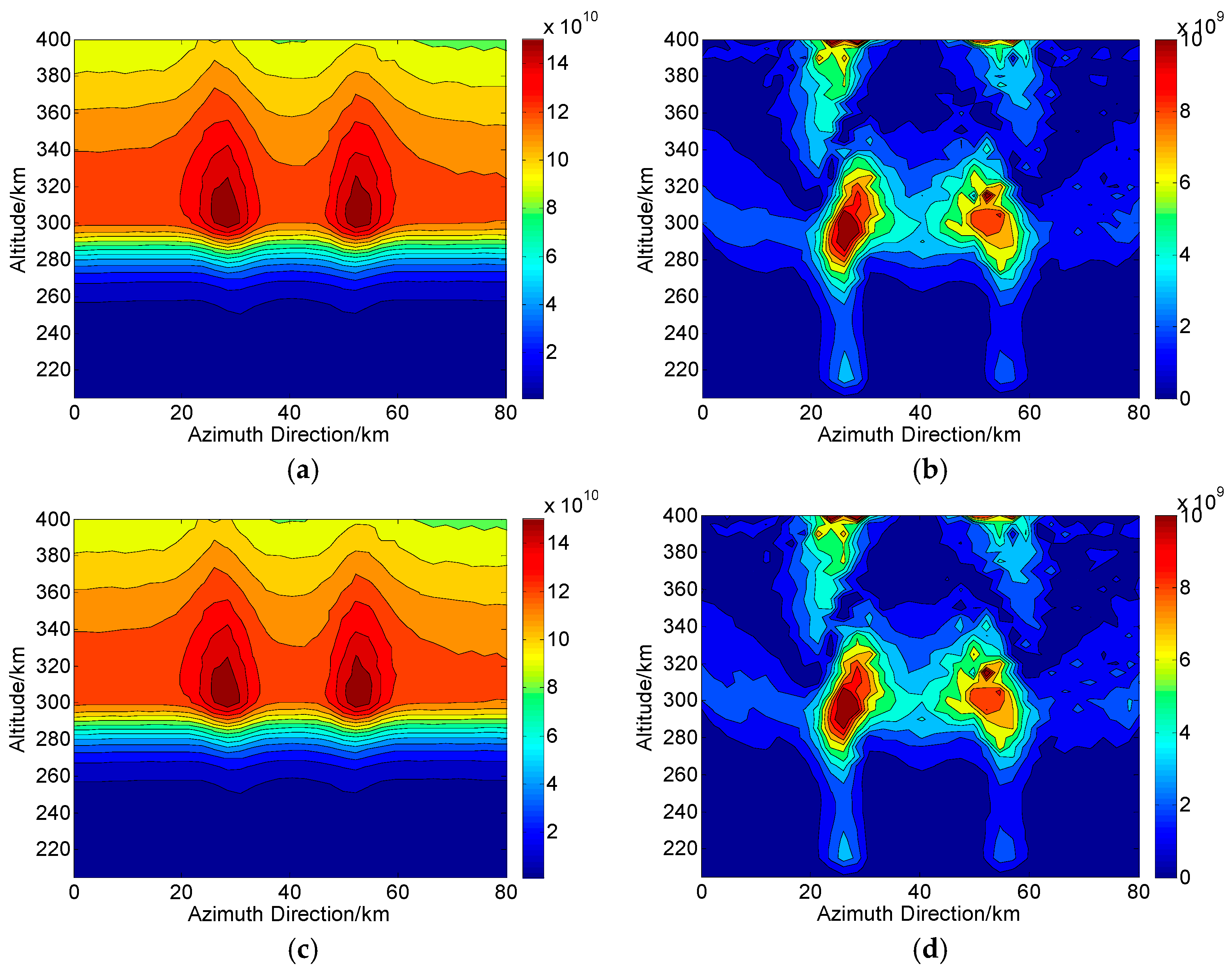
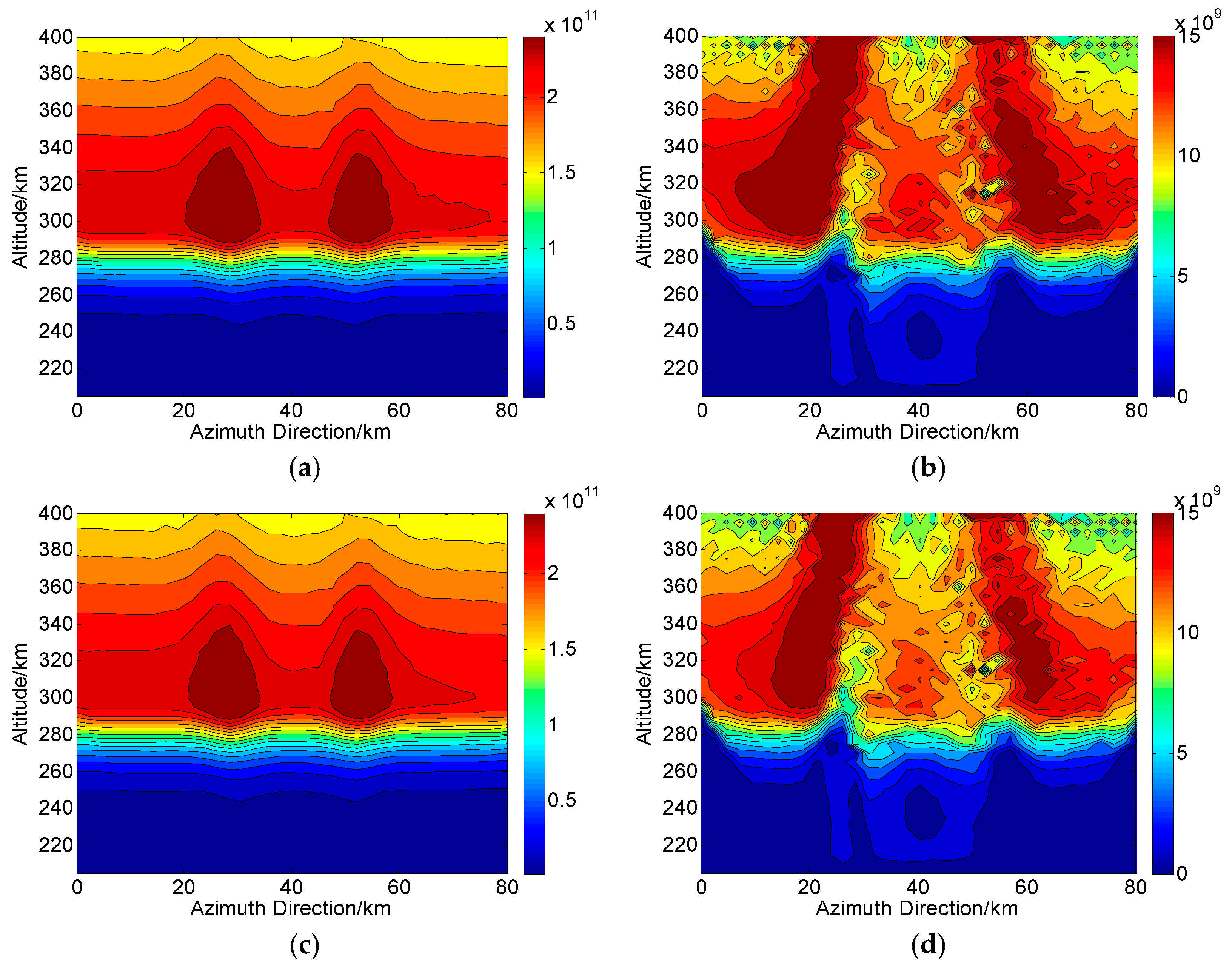
Figure 9.
Two-dimensional CIT reconstructions under the condition of channel phase imbalance () in Changbai. (a,c) are the reconstructed results based on and , respectively. (b,d) are the corresponding absolute deviations between the true and reconstructed results. The unit of the electron density is .
Figure 10.
Two-dimensional CIT reconstructions under the condition of channel phase imbalance () in Qingdao. (a,c) are the reconstructed results based on and , respectively. (b,d) are the corresponding absolute deviations between the true and reconstructed results. The unit of the electron density is .
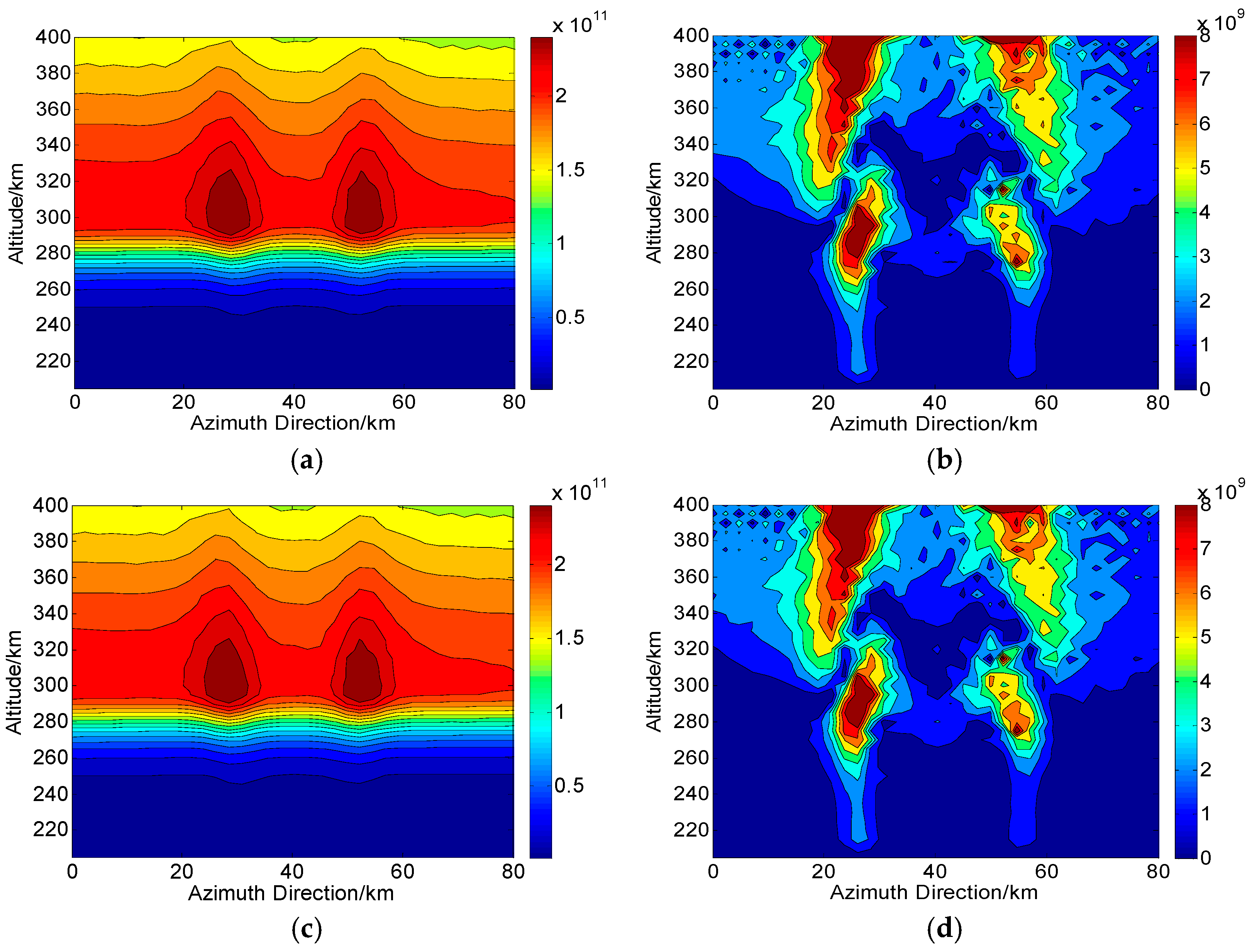
Figure 11.
Two-dimensional CIT reconstructions under the condition of channel phase imbalance () in Changbai. (a,c) are the reconstructed results based on and , respectively. (b,d) are the corresponding absolute deviations between the true and reconstructed results. The unit of the electron density is .
Figure 12.
Two-dimensional CIT reconstructions under the condition of channel phase imbalance () in Qingdao. (a,c) are the reconstructed results based on and , respectively. (b,d) are the corresponding absolute deviations between the true and reconstructed results. The unit of the electron density is .
Figure 13.
Two-dimensional CIT reconstructions under the condition of channel amplitude imbalance in Changbai ( is used). (a,c) are the reconstructed results with and , respectively. (b,d) are the corresponding absolute deviations between the true and reconstructed results. The unit of the electron density is .
Figure 14.
Two-dimensional CIT reconstructions under the condition of channel amplitude imbalance in Qingdao ( is used). (a,c) are the reconstructed results with and , respectively. (b,d) are the corresponding absolute deviations between the true and reconstructed results. The unit of the electron density is .
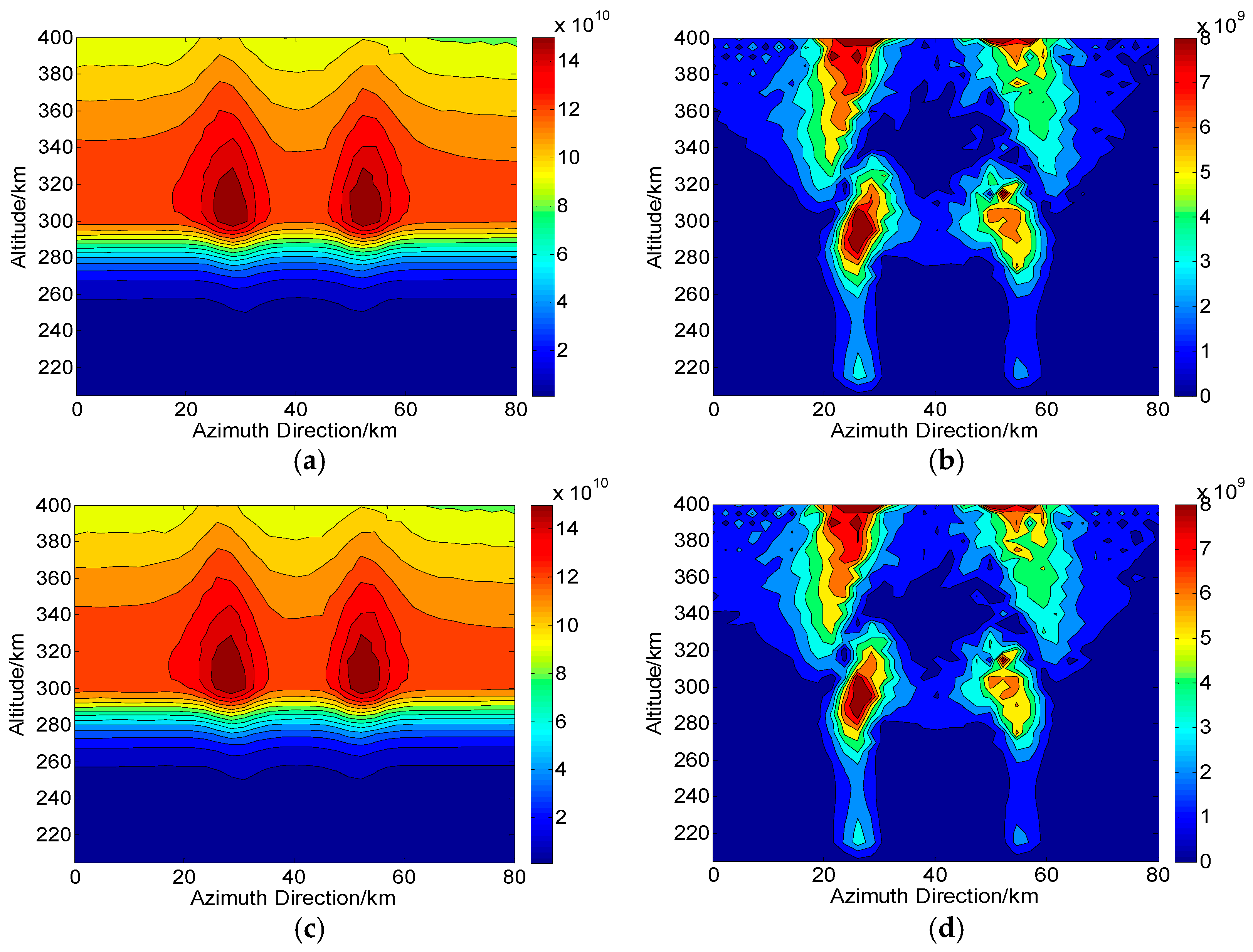
Figure 15.
Two-dimensional CIT reconstructions under the condition of crosstalk in Changbai ( is used). (a,c) are the reconstructed results with and , respectively. (b,d) are the corresponding absolute deviations between the true and reconstructed results. The unit of the electron density is .
Figure 15.
Two-dimensional CIT reconstructions under the condition of crosstalk in Changbai ( is used). (a,c) are the reconstructed results with and , respectively. (b,d) are the corresponding absolute deviations between the true and reconstructed results. The unit of the electron density is .
Figure 16.
Two-dimensional CIT reconstructions under the condition of crosstalk in Qingdao. (a) ( is used) and (c) ( is used) are the reconstructed results with and , respectively. (b,d) are the corresponding absolute deviations between the true and reconstructed results. The unit of the electron density is .
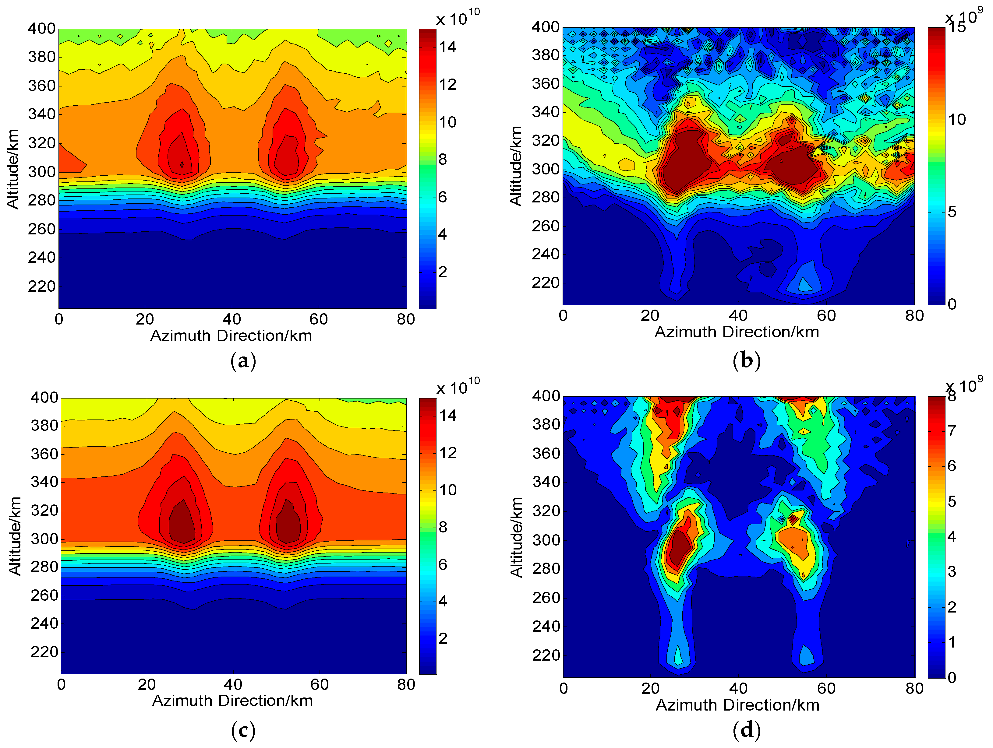
Figure 17.
Two-dimensional CIT reconstructions under the condition of joint errors. (a) ( is used) and (c) ( is used) are the reconstructed results in areas of Changbai and Qingdao, respectively. (b,d) are the corresponding absolute deviations between the true and reconstructed results. The unit of the electron density is .
Table 1.
RMS error () under the condition of system noise.
Table 1.
RMS error () under the condition of system noise.
| SNR (dB) | RMS Error (%) |
|---|
| Changbai | Qingdao |
|---|
| | | | | |
|---|
| 5 | 19.1023 | 866.7750 | 3.1956 | 10.6599 | 457.1695 | 14.1860 |
| 10 | 9.2369 | 475.1484 | 1.4204 | 4.0307 | 237.6931 | 7.8032 |
| 15 | 3.4335 | 239.2308 | 0.8279 | 1.3728 | 109.9127 | 4.0608 |
| 20 | 1.5564 | 109.0368 | 0.3182 | 0.5284 | 44.7311 | 1.9436 |
| 25 | 0.9041 | 44.1177 | 0.2153 | 0.2032 | 16.1787 | 1.4127 |
| 30 | 0.3327 | 15.9300 | 0.0991 | 0.1384 | 5.4124 | 0.5717 |
Table 2.
Bias () under the condition of system noise.
Table 2.
Bias () under the condition of system noise.
| SNR (dB) | Bias (%) |
|---|
| Changbai | Qingdao |
|---|
| | | | | |
|---|
| 5 | 18.6803 | −858.3574 | 1.1071 | 7.8405 | −452.2203 | 7.8584 |
| 10 | 8.0336 | −469.8182 | −0.9973 | 3.2375 | −234.7492 | 3.3109 |
| 15 | 3.1830 | −235.7411 | 0.2154 | 1.2264 | −108.1120 | 1.3629 |
| 20 | 1.1940 | −107.1453 | −0.1585 | 0.5594 | −43.7774 | 0.6791 |
| 25 | 0.3286 | −43.1128 | −0.0424 | 0.0342 | −15.7346 | 0.2223 |
| 30 | 0.1523 | −15.4490 | 0.0385 | −0.0017 | −5.2271 | 0.0380 |
Table 3.
SD () under the condition of system noise.
Table 3.
SD () under the condition of system noise.
| SNR (dB) | SD (%) |
|---|
| Changbai | Qingdao |
|---|
| | | | | |
|---|
| 5 | 8.0833 | 121.1693 | 2.9652 | 1.2226 | 65.3801 | 17.1186 |
| 10 | 5.3539 | 70.6254 | 1.5441 | 0.8802 | 37.3999 | 7.5438 |
| 15 | 2.1559 | 39.2181 | 0.7358 | 0.4353 | 19.7724 | 4.6861 |
| 20 | 1.0907 | 20.4720 | 0.3469 | 0.2412 | 9.2965 | 1.7415 |
| 25 | 0.5715 | 9.5487 | 0.1984 | 0.1454 | 3.7366 | 1.1294 |
| 30 | 0.2959 | 3.8175 | 0.1311 | 0.1013 | 1.3163 | 0.5045 |
Table 4.
RMS error () under the condition of channel phase imbalance.
Table 4.
RMS error () under the condition of channel phase imbalance.
| Channel Phase Imbalance (°) | RMS Error (%) |
|---|
| Changbai | Qingdao |
|---|
| | | | | |
|---|
| 5 | 1.5075 | 1.5863 | 5.0152 | 0.4340 | 0.4644 | 5.7890 |
| 10 | 3.6991 | 3.9594 | 9.2409 | 1.5537 | 1.6645 | 7.4793 |
| 15 | 6.6352 | 7.2038 | 13.9008 | 3.3994 | 3.6423 | 9.8274 |
| 20 | 10.4286 | 11.4409 | 19.5022 | 6.0230 | 6.4697 | 13.0879 |
Table 5.
Bias () under the condition of channel phase imbalance.
Table 5.
Bias () under the condition of channel phase imbalance.
| Channel Phase Imbalance (°) | Bias (%) |
|---|
| Changbai | Qingdao |
|---|
| | | | | |
|---|
| 5 | −1.4987 | −1.5859 | −4.8996 | −0.4337 | −0.4643 | −5.7350 |
| 10 | −3.6691 | −3.9582 | −9.0977 | −1.5528 | −1.6643 | −7.4330 |
| 15 | −6.6716 | −7.2012 | −13.7565 | −3.3974 | −3.6420 | −9.7901 |
| 20 | −10.3174 | −11.4362 | −19.3646 | −6.0199 | −6.4692 | −13.0582 |
Table 6.
SD () under the condition of channel phase imbalance.
Table 6.
SD () under the condition of channel phase imbalance.
| Channel Phase Imbalance (°) | SD (%) |
|---|
| Changbai | Qingdao |
|---|
| | | | | |
|---|
| 5 | 0.1620 | 0.0371 | 1.0709 | 0.0180 | 0.0096 | 0.7895 |
| 10 | 0.4708 | 0.0983 | 1.6208 | 0.0523 | 0.0251 | 0.8311 |
| 15 | 0.9164 | 0.1910 | 1.9986 | 0.1175 | 0.0482 | 0.8558 |
| 20 | 1.5199 | 0.3261 | 2.3139 | 0.1954 | 0.0809 | 0.8814 |
Table 7.
RMS error () under the condition of channel amplitude imbalance.
Table 7.
RMS error () under the condition of channel amplitude imbalance.
| Channel Amplitude Imbalance (dB) | RMS Error (%) |
|---|
| Changbai | Qingdao |
|---|
| | | | | |
|---|
| 0.1 | 0.1525 | 0.2570 | 0.0066 | 0.0688 | 0.0659 | 0.0066 |
| 0.2 | 0.2958 | 0.5045 | 0.0266 | 0.1233 | 0.1187 | 0.0266 |
| 0.3 | 0.4270 | 0.7358 | 0.0594 | 0.1632 | 0.1570 | 0.0594 |
| 0.4 | 0.5509 | 0.9570 | 0.1060 | 0.1890 | 0.1820 | 0.1060 |
| 0.5 | 0.6630 | 1.1639 | 0.1654 | 0.1982 | 0.1933 | 0.1652 |
Table 8.
Bias () under the condition of channel amplitude imbalance.
Table 8.
Bias () under the condition of channel amplitude imbalance.
| Channel Amplitude Imbalance (dB) | Bias (%) |
|---|
| Changbai | Qingdao |
|---|
| | | | | |
|---|
| 0.1 | −0.1198 | −0.2539 | −0.0066 | −0.0684 | −0.0655 | −0.0066 |
| 0.2 | −0.2281 | −0.4980 | −0.0266 | −0.1225 | −0.1178 | −0.0266 |
| 0.3 | −0.3215 | −0.7257 | −0.0594 | −0.1617 | −0.1555 | −0.0594 |
| 0.4 | −0.4041 | −0.9430 | −0.1060 | −0.1868 | −0.1796 | −0.1058 |
| 0.5 | −0.4738 | −1.1459 | −0.1654 | −0.1949 | 0.1897 | −0.1652 |
Table 9.
SD () under the condition of channel amplitude imbalance.
Table 9.
SD () under the condition of channel amplitude imbalance.
| Channel Amplitude Imbalance (dB) | SD (%) |
|---|
| Changbai | Qingdao |
|---|
| | | | | |
|---|
| 0.1 | 0.0945 | 0.0401 | 0.00001 | 0.0072 | 0.0074 | 0.00001 |
| 0.2 | 0.1884 | 0.0811 | 0.00001 | 0.0142 | 0.0149 | 0.00001 |
| 0.3 | 0.2811 | 0.1216 | 0.00002 | 0.0222 | 0.0222 | 0.00002 |
| 0.4 | 0.3745 | 0.1629 | 0.00002 | 0.0281 | 0.0296 | 0.00003 |
| 0.5 | 0.4639 | 0.2042 | 0.00002 | 0.0356 | 0.0370 | 0.00005 |
Table 10.
RMS error () under the condition of crosstalk.
Table 10.
RMS error () under the condition of crosstalk.
| Crosstalk (dB) | RMS Error (%) |
|---|
| Changbai | Qingdao |
|---|
| | | | | |
|---|
| −15 | 8.8421 | 7.6382 | 7.7358 | 6.2014 | 6.0407 | 2.5106 |
| −20 | 3.7897 | 2.8994 | 2.9776 | 1.9464 | 1.8950 | 1.1415 |
| −25 | 1.7467 | 1.1683 | 1.2207 | 0.5906 | 0.5700 | 0.9784 |
| −30 | 0.8633 | 0.5115 | 0.5437 | 0.1698 | 0.1623 | 0.6808 |
| −35 | 0.4496 | 0.2430 | 0.2621 | 0.0437 | 0.0413 | 0.4264 |
Table 11.
Bias () under the condition of crosstalk.
Table 11.
Bias () under the condition of crosstalk.
| Crosstalk (dB) | Bias (%) |
|---|
| Changbai | Qingdao |
|---|
| | | | | |
|---|
| −15 | 8.6232 | 7.5837 | 7.6724 | 5.4012 | 5.4406 | −1.8124 |
| −20 | 3.5849 | 2.8467 | 2.9162 | 1.6463 | 1.6949 | −1.5488 |
| −25 | 1.5885 | 1.1245 | 1.1700 | 0.5925 | 0.5669 | −0.8016 |
| −30 | 0.7551 | 0.4788 | 0.5064 | 0.1684 | 0.1612 | −0.6044 |
| −35 | 0.3811 | 0.2207 | 0.2369 | 0.0426 | 0.0416 | −0.3885 |
Table 12.
SD () under the condition of crosstalk.
Table 12.
SD () under the condition of crosstalk.
| Crosstalk (dB) | SD (%) |
|---|
| Changbai | Qingdao |
|---|
| | | | | |
|---|
| −15 | 1.9561 | 0.9114 | 0.9888 | 1.1464 | 1.1382 | 1.0981 |
| −20 | 1.2295 | 0.5506 | 0.6017 | 0.8232 | 0.8218 | 0.7813 |
| −25 | 0.7268 | 0.3172 | 0.3481 | 0.1390 | 0.1224 | 0.5612 |
| −30 | 0.4186 | 0.1800 | 0.1980 | 0.0832 | 0.0681 | 0.3135 |
| −35 | 0.2387 | 0.1017 | 0.1120 | 0.0393 | 0.0385 | 0.1757 |
Table 13.
The performances of FR estimators under the condition of joint errors.
Table 13.
The performances of FR estimators under the condition of joint errors.
| Performances | Changbai | Qingdao |
|---|
| | | | | |
|---|
| RMS error (%) | 3.6572 | 262.1338 | 1.8965 | 1.4348 | 120.5995 | 6.6420 |
| Bias (%) | 3.5491 | −258.7012 | −1.7362 | 1.3959 | −118.7056 | −5.5683 |
| SD (%) | 2.9604 | 42.3003 | 0.8634 | 0.5181 | 21.2925 | 4.9092 |


