Abstract
Fire detection based on multi-temporal remote sensing data is an active research field. However, multi-temporal detection processes are usually complicated because of the spatial and temporal variability of remote sensing imagery. This paper presents a spatio-temporal model (STM) based forest fire detection method that uses multiple images of the inspected scene. In STM, the strong correlation between an inspected pixel and its neighboring pixels is considered, which can mitigate adverse impacts of spatial heterogeneity on background intensity predictions. The integration of spatial contextual information and temporal information makes it a more robust model for anomaly detection. The proposed algorithm was applied to a forest fire in 2009 in the Yinanhe forest, Heilongjiang province, China, using two-month HJ-1B infrared camera sensor (IRS) images. A comparison of detection results demonstrate that the proposed algorithm described in this paper are useful to represent the spatio-temporal information contained in multi-temporal remotely sensed data, and the STM detection method can be used to obtain a higher detection accuracy than the optimized contextual algorithm.
1. Introduction
Forest fires are natural ecosystem processes that have a significant impact on environment protection, ecosystem equilibria, and climate change [1,2]. Early detection of forest fires is helpful for monitoring the high rate of fire spread, instantaneous fire radiative energy, smoldering ratio, and consequences of biomass burning for climate and ecosystem functions. Remote sensing has been widely used in forest fire detection. The use of thermal infrared images is a well-known technique to detect actively burning fires. At present, most satellite-based fire detection algorithms are based on the detection of thermal anomalies produced by the high temperatures of burning fuels in midwave infrared (MWIR) and longwave infrared (LWIR) bands. Those algorithms can be divided into single-date and multi-temporal detection methods according to the number of source images.
Single-date fire detection methods are commonly classified as either fixed-threshold or contextual algorithms [3]. Fixed-threshold algorithms regard a pixel as an active fire pixel if the brightness temperature (BT) or radiance in the MWIR and LWIR bands exceeds pre-specified thresholds [4,5,6,7]. In contrast, contextual algorithms first label a pixel as a “potential active fire” with a similar series of fixed thresholds. The tests are then used to verify whether the pixel is a “true fire pixel” or a “false fire pixel” by comparing the observed value with the background intensity, which is predicted by averaging the intensities over the neighboring pixels [8,9,10,11,12]. If the observed value is sufficiently higher than the ambient background intensity, the pixel is identified as a fire pixel. For fixed-threshold and contextual algorithms, the optimal thresholds are difficult to determine because of the variability of the natural background in the time and spatial domains. It is impossible to detect all the active burning pixels, especially for small fires.
Unlike fixed-threshold or contextual algorithms, multi-temporal fire detection methods focus on exploiting the multi-temporal nature of data in a thermal anomaly detection process. For example, Laneve et al. [13] developed a multi-temporal detection algorithm for Spinning Enhanced Visible and Infrared Imager (SEVIRI) images that detects fire pixels by comparing successive observations. Koltunov and Ustin [14] proposed a non-linear Dynamic Detection Model (DDM) for multi-temporal thermal infrared images. Mazzeo et al. [15] applied a robust satellite technique (RST) to forest fire detection in near real time. They proposed a new index, which they called the Absolute Local Index of Change of the Environment (ALICE), as a quantitative standard to monitor forest fire pixels. Roberts and Wooster [16] developed a multi-temporal Kalman filter approach for geostationary active fire detection. Although these methods performed well on test data, potential limitations, including background surface properties, weather influence, and missing pixel values, have hindered further development. In addition, most existing multi-temporal fire detection algorithms do not take full advantage of spatial contextual information.
In this paper, we propose a novel spatio-temporal model that uses spatial contextual and temporal information to detect active forest fires. The spatio-temporal model (STM) based forest fire detection method relies on the strong correlation between an inspected pixel and its spatial neighborhood. Spatial correlation is used in STM for predicting the background intensity of the pixel. In addition, to make a more robust fire detection method, the STM method adds temporal information to the anomaly detection by assigning different weights to the inspection image and previous images. A test area from China’s Heilongjiang province was used to validate the STM method. A fire broke out in the Yinanhe forest on 27 April 2009, and it was contained on 11 May 2009. Thirteen HJ-1B/IRS images were used for this work. The fire detection results were evaluated on a validation set and compared with the results of the contextual algorithm.
2. Study Area and Data
2.1. Study Area
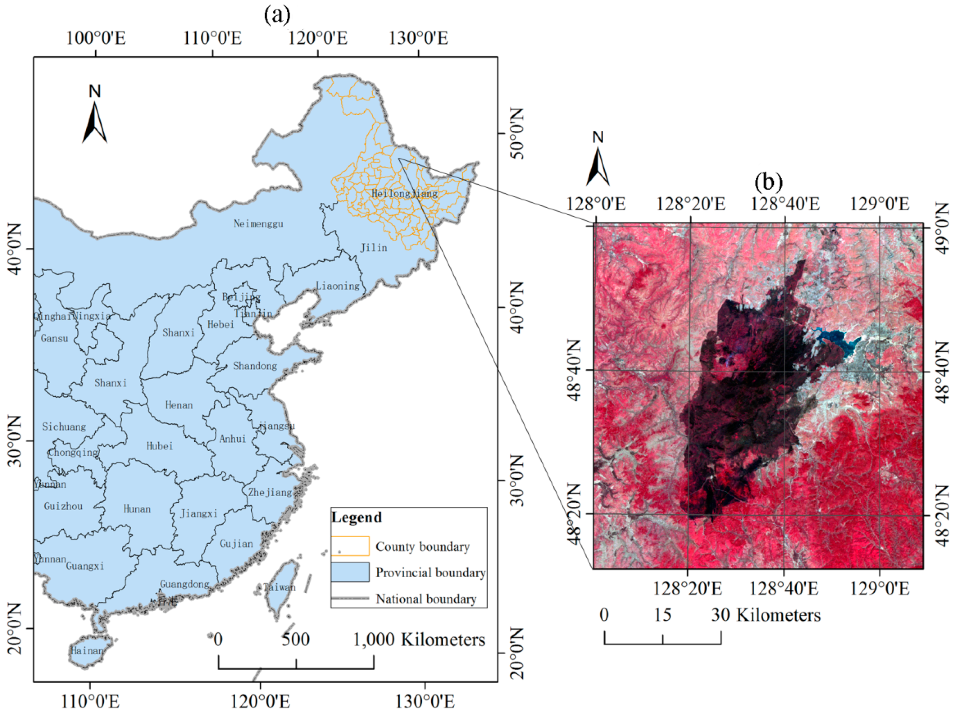
The Yinanhe forest is located in the northern part of Heilongjiang Province, China. The Yinanhe forest belongs to the subtemperate zone and possesses a humid climate, with an average annual temperature of −2 °C, a maximum temperature of 38 °C, and a minimum temperature of −42 °C. The average elevation is 656 m. The vegetation belongs to the Lesser Hinggan flora and primarily includes cold hardy plants. On 27 April 2009, a forest fire broke out in the Yinanhe forest. The fire was located at 48°41′N latitude and 128°12′E longitude (Figure 1).

Figure 1.
The location of the study area (a); and the 30-m HJ-1B CCD false color image (R: Near Infrared (NIR), G: Red, B: Green) acquired on 11 May 2009 (b).
2.2. HJ-1B Satellite Data
HJ-1B is a small optical satellite that is part of the “Environment and Disaster Monitoring and Forecasting with a Small Satellite Constellation (HJ-1)” project in China. The HJ-1 satellite system is dedicated to the study of ground environment changes and disaster monitoring. HJ-1B carries two charge-coupled device (CCD) cameras and an infrared camera sensor (IRS). The sensor parameters are shown in Table 1 [17,18].

Table 1.
HJ-1B satellite sensor parameters.
The source data used in this paper are IRS infrared data, i.e., the Near Infrared band (NIR, band 5), Shortwave Infrared band (SWIR, band 6), MWIR band (band 7) and LWIR band (band 8). Compared to the Moderate Resolution Imaging Spectroradiometer (MODIS), IRS in HJ-1B is more appropriate for detecting small and cool fire spots with finer pixel resolutions of 150 m/300 m and a temperature saturation point of 500 K. The revisit frequency of 4 days also meets the time requirement for forest fire monitoring. Wang et al. [19] statistically analyzed and compared the BTs of the HJ-1B and MODIS thermal infrared bands (band 7 vs. band 21). They found that the main BT distribution range of HJ-1B is narrower than that of the MODIS data, although it includes more random noise.
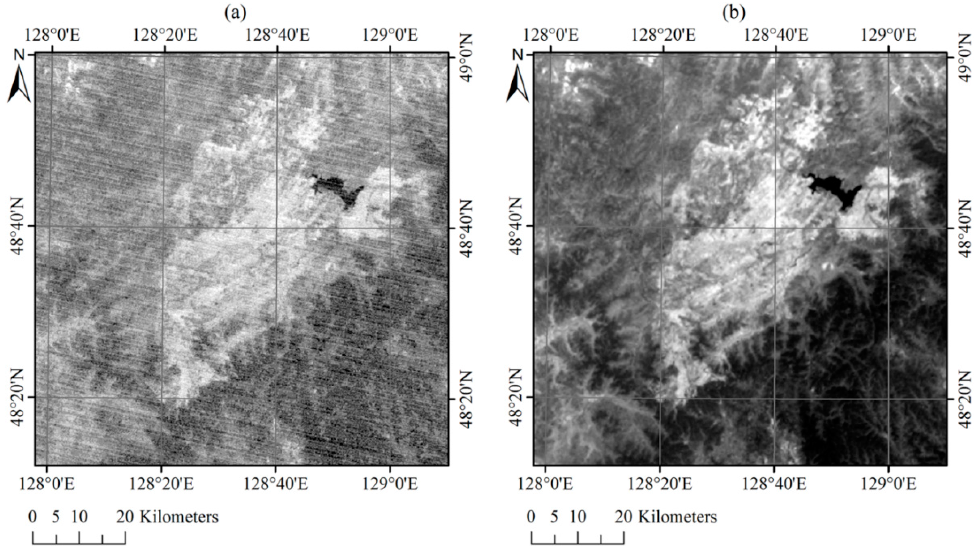
The HJ-1B/IRS data used in this paper include 13 images acquired in 2009. The data were downloaded from the China Centre for Resources Satellite Data and Application website [17]. The temporal distribution of the images is shown in Figure 2, and two BT images from band 7 and band 8 acquired on 22 May 2009 are shown in Figure 3. Although the revisit cycle of HJ-1B is four days, we can obtain two available images over a two-day period because study area is covered in the overlapping region of the two images photographed in different tracks.

Figure 2.
Temporal distribution of the images used from the two months. Each spot represents an acquired image.

Figure 3.
Brightness temperature (BT) images from band 7 (a) and band 8 (b) acquired on 22 May 2009.
2.3. Ground Reference Data
Because it is difficult to obtain reliable ground truth data to evaluate forest fire detection performance, researchers often use ancillary remote sensed data [20,21] or smoke plumes from high-resolution images [22] to verify forest fire products. In this study, we obtained ground-based data using visual image interpretation. We made a false color composite image (Figure 4a) using band 7, band 6, and band 5 of the IRS data to serve as a primary reference. The HJ-1B CCD images (Figure 4b) and the official MODIS active fire products (MOD14A1) (Figure 4c) were also referenced. MOD14A1, which offers global daily active fire detections at a 1-km resolution, were downloaded from the Level 1 and Atmosphere Archive and Distribution System (LAADS) website [23]. The ground reference data are shown in Figure 5. The active fire can be found in the four satellite images acquired on 28 April, 29 April, 3 May, and 11 May.
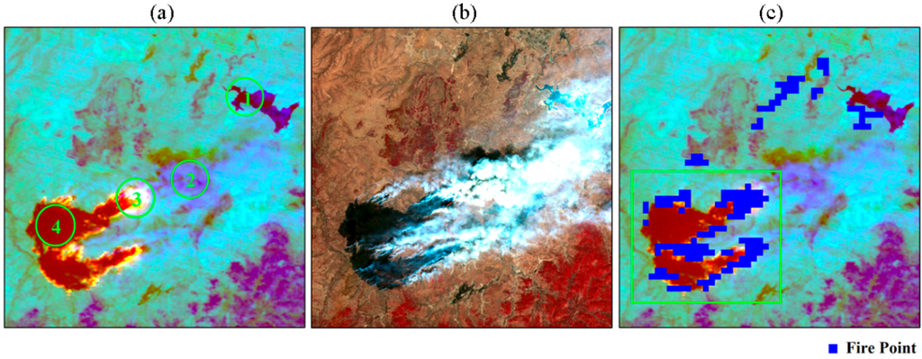
Figure 4.
Reference images acquired on 29 April 2009: (a) HJ-1B IRS false color image (R: band 7, G: band 6, B: band 5), dark blue represents water (green circle 1), blue represents smoke (green circle 2), bright red represents active fire (green circle 3) and reddish brown represents post fire (green circle 4); (b) HJ-1B CCD false color image (R: band 4, G: band 3, B: band 2); and (c) MODIS fire product.
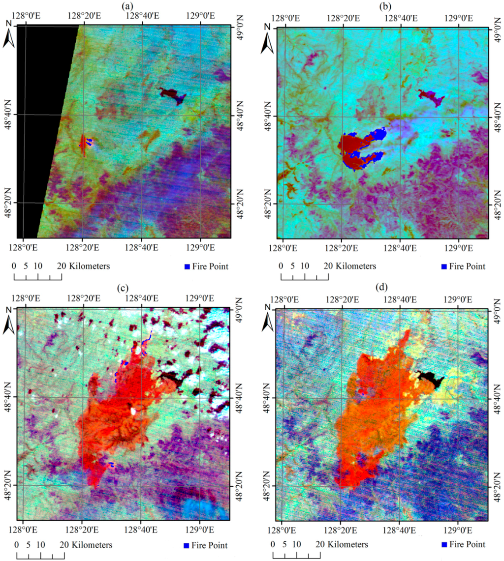
Figure 5.
Ground reference data showing the evolution of the fire fronts in the Yinanhe forest on: 28 April 2009 (a); 29 April 2009 (b); 3 May 2009 (c); and 11 May 2009 (d).
3. Methodology
3.1. Contextual Algorithm
Before presenting our proposed spatio-temporal model, we will begin with an introduction to the contextual method. The spatial contextual method combines a series of absolute threshold tests to identify cloud, water and potential fire pixels. It then uses contextual tests to identify fires among the potential fire pixels. Finally, it uses additional algorithms to filter out false positives. Two contextual tests (Equations (1) and (2)) are among the key parts of the method. They attempt to predict the background BT of a potential fire pixel by calculating the average intensity of the valid neighboring pixels in a window. The valid neighboring pixels are defined as those pixels that: (i) contain usable observations; (ii) are located on land; (iii) are not cloud-contaminated; and (iv) are not background fire pixels [8]. The mean absolute deviation is also used to detect fire in the thresholds.
where ΔT = T7 − T8; T7 and T8 denote BTs from band 7 and band 8 for the inspected pixel, respectively; μ7 and Δμ denote the mean values of T7 and ΔT of valid neighboring pixels, respectively; δ7 and Δδ denote their mean absolute deviations; and λ1 and λ2 are learning parameters that determine the thresholds.
Additional details on the implementation of the contextual algorithm for HJ-IRS data are given in [24].
3.2. Overview of the Improved Algorithm
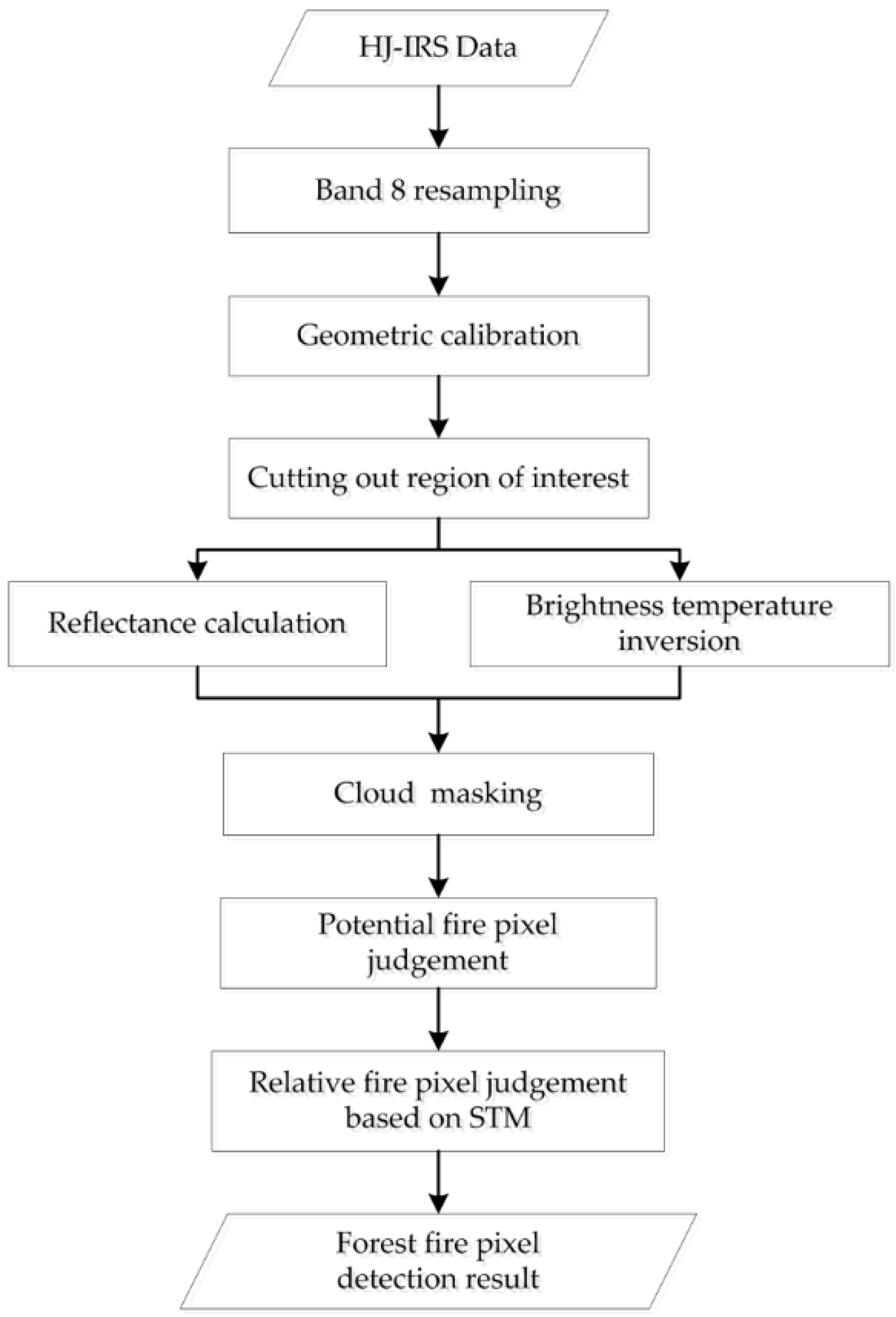
As with the spatial contextual algorithm, the forest fire detection algorithm proposed in this study includes four major steps: data preprocessing, cloud masking, potential fire pixel judgment, and relative fire pixel judgment based on STM. A STM method workflow is illustrated in Figure 6.
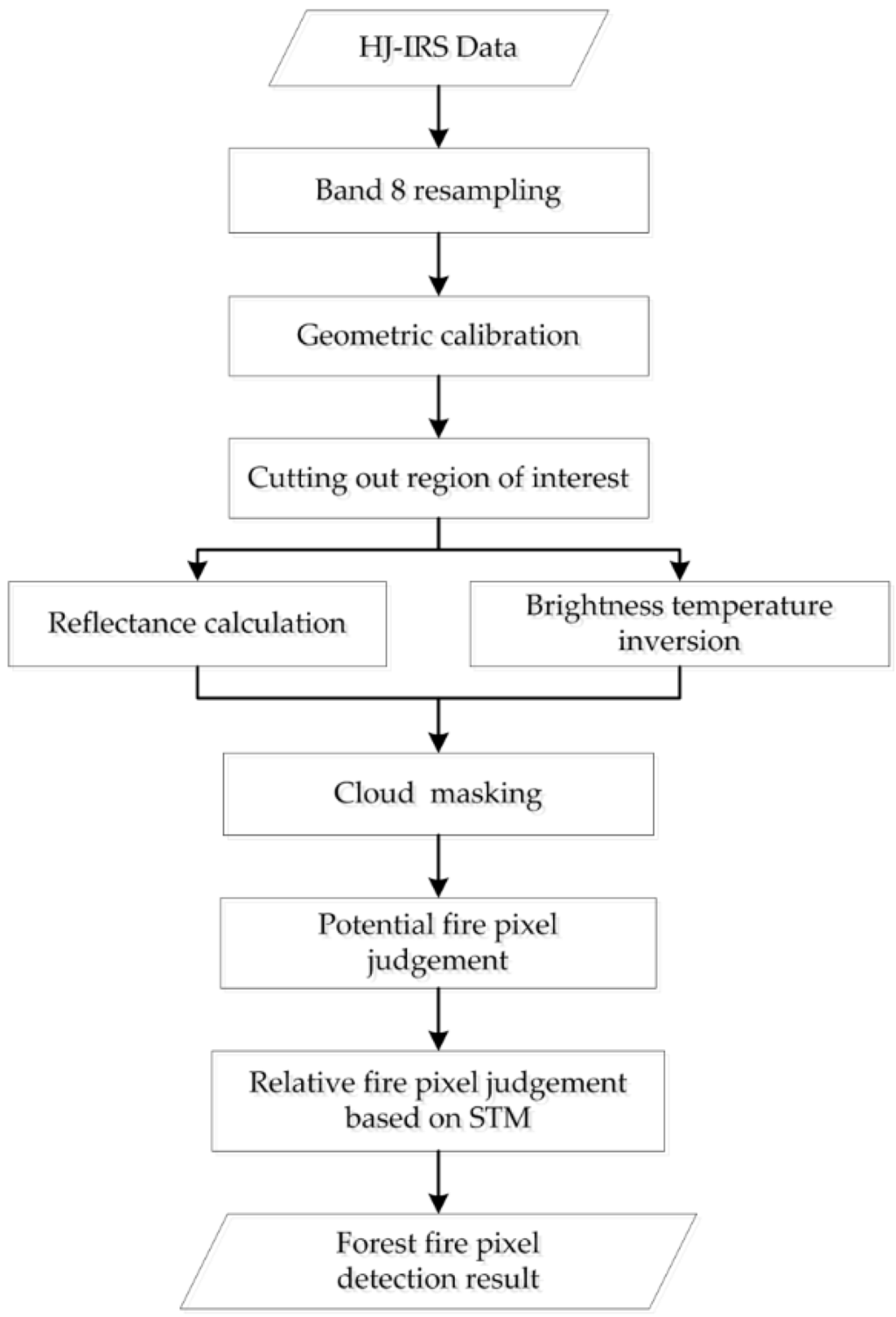
Figure 6.
Workflow of the spatio-temporal model (STM) based forest fire detection method.
3.2.1. Data Preprocessing
The preprocessing procedure for the IRS images includes the following processes. (I) Resampling: Because the pixel resolution of the band 8 IRS images is 300 m, whereas the resolutions of the three other (band 5, band 6, band 7) are 150 m, we converted band 8 to 150 m by nearest-neighbor resampling, which assigns the digital number of the closest input pixel to the corresponding output pixel; (II) Geometric calibration: The image acquired on 1 April was chosen as the reference image, and the other images were corrected using geometric calibration with a correction error of 0.5 pixels or less; (III) Cutting out the region-of-interest (ROI): A 90 × 90 km2 square region (600 × 600 pixels for HJ-IRS) was chosen as the validation site. A ROI between 48°11′49.0″N and 49°0′45.0″N latitude and 127°57′41.8″E to 129°10′39.4″E longitude covered the entire fire zone in the Yinanhe forest; (IV) Reflectance calculation and brightness temperature inversion: This process was used to convert the digital number (DN) values to radiances, reflectance and BTs. According to the absolute radiometric calibration tests conducted by the China Centre for Resources Satellite Data and Application, the DN values for bands 5 were converted to radiance values using Equation (3), whereas the DN values for bands 7 and 8 were converted to radiance values using Equation (4). The radiances for band 5 were converted to reflectance using Equation (5). The radiances for bands 7 and 8 were converted to BTs using Equation (6), which was derived using Planck’s law.
where L is the radiance, DN is the observed value, g is the gain coefficient, and b is the offset, which we obtained from the data item description of HJ-1B. In Equation (5), R is the reflectance, ds is the distance between the earth and the sun, E is the mean solar spectral irradiance, and θ is the solar zenith angle. In Equation (6), T is the brightness temperature, is the center wavelength, and C1 and C2 are constants whose values are 3.741775 × 10⁻²² Wm3·μ−1 and 0.0143877 mK, respectively, according to [25].
3.2.2. Cloud Masking
In the STM method, the cloud-contaminated pixels usually have a negative effect on the anomaly detection results. It was therefore necessary to remove the cloud-covered pixels from the IRS images. Clouds have strong reflectivity in NIR band and low BTs in LWIR band. The following Equations are the rules for extracting clouds [26]:
where R5 is the reflectance in band 5, and T8 is BT in band 8 of the IRS image. The pixels that satisfied both conditions were masked off as clouds.
3.2.3. Potential Fire Pixel Judgment
MWIR band of HJ-IRS is sensitive to BT changes and can be used to eliminate obvious non-fire pixels. According to [24], a pixel is identified as a potential active fire pixel if the BT of band 7 meets the criterion T7 > 325 K in the daytime. In our study, the HJ-1B satellite passing time was approximately 10:30 a.m.
3.2.4. Relative Fire Pixel Judgment Based on STM
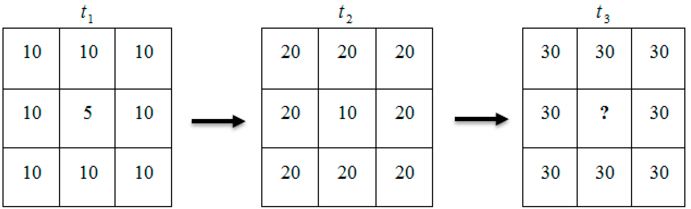
In the contextual algorithm, potential fire pixels whose observed BT values were significantly different from the background intensities (predicted BT values) were considered to be actual fire points. Thus, the background BT prediction played an important role in the fire detection. The mean value of the valid neighboring pixels was regarded as the background intensity in the contextual algorithms. However, it was occasionally difficult to use that value to indicate the characteristics of the background because of spatial heterogeneity. For example, the mean value in frame t3 (Figure 7) cannot be taken as the background intensity of the question mark because 15 is a better choice than 30 according to the data distribution in frames t1 and t2. It is obvious that the strong correlations between the center grid and its neighboring grids in frames t1 and t2 are helpful for predicting the background intensity of the center grid in frame t3.
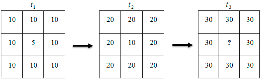
Figure 7.
Background intensity prediction for frames with spatial heterogeneity.
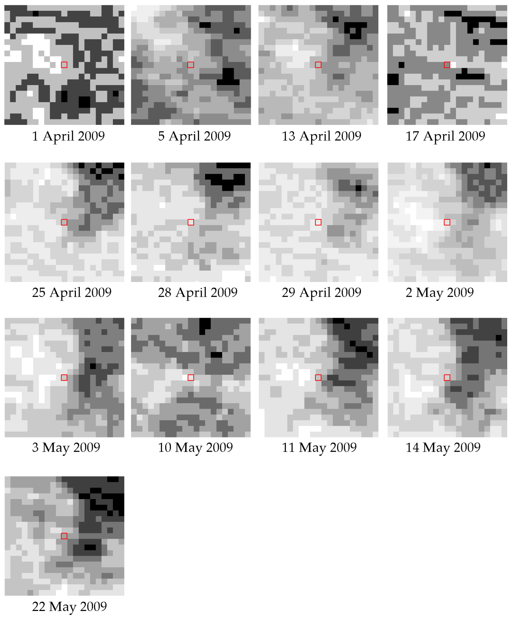
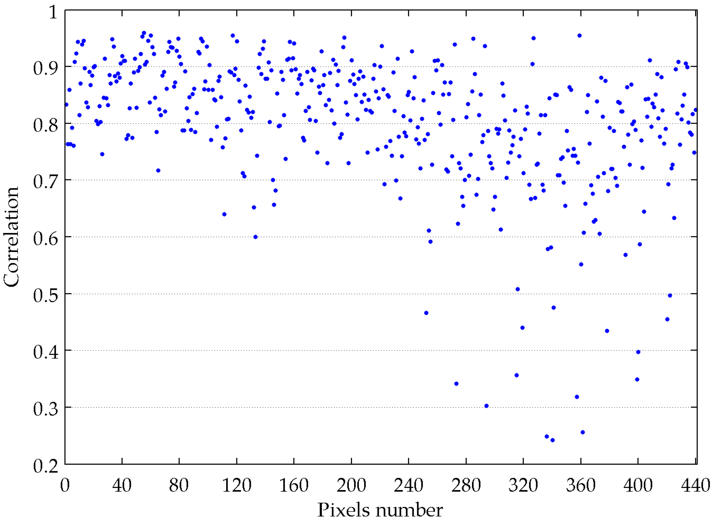
Spatial heterogeneity is a common phenomenon in remote sensing images. Figure 8 shows the BT changes of an inspected pixel and its neighboring pixels over time. The size of each image is 21 × 21, and we had 441 time series with lengths of 13 frames. The correlation coefficients between the inspected time series and the neighboring time series are shown in Figure 9. The mean of the correlation coefficients was 0.8021, which indicates a high correlation. Thus, a spatio-temporal model can be built using the correlation relationship between the pixels to predict the background intensity with multi-temporal images.

Figure 8.
BTs distribution from band 7 for 13 IRS images. The red pixel is the inspected pixel in the window.
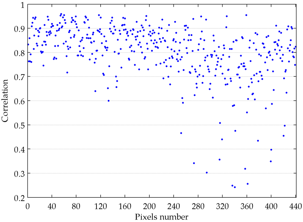
Figure 9.
Correlation coefficients between the inspected time series and the neighboring time series.
Background BT Prediction
In the proposed model, let be the spatial context of pixel , where is the window size, is the index of a pixel in the image, and represents the BT value at pixel in the image acquired at time . The spatial relationship between and each of its neighboring pixels in is simply defined by the following equation:
where , and N is the number of images used in the fire detection algorithm. The spatial relationship is updated using
where is the spatial relationship computed by Equation (9) in the n-th image, , , and is a learning parameter that controls the weights of the images acquired at different time points. In particular, the spatial relationship between the inspected pixel and its neighboring pixels is only decided by its previous image when , and the previous one does not contribute to the spatial relationship calculation when . In STM, an ideal hypothesis is that the spatial relationship remains unchanged over time. The spatial relationship of the current pixel should be decided by all of the previous images to meet this requirement. Thus, should not be larger than 0.5. To obtain satisfactory fire pixels detection results, is a good choice.
The background BT can then be computed by
where is regarded as the background BT at time . For the first image (n = 1), the mean value of the valid neighboring pixels is regarded as the background BT.
Importantly, the pixels in the background BT calculation must be valid. In this study, the valid neighboring pixels were defined as those that: (i) contained usable observations; (ii) were not contaminated by clouds; and (iii) were not background fire pixels.
Integration of Spatial and Temporal Information
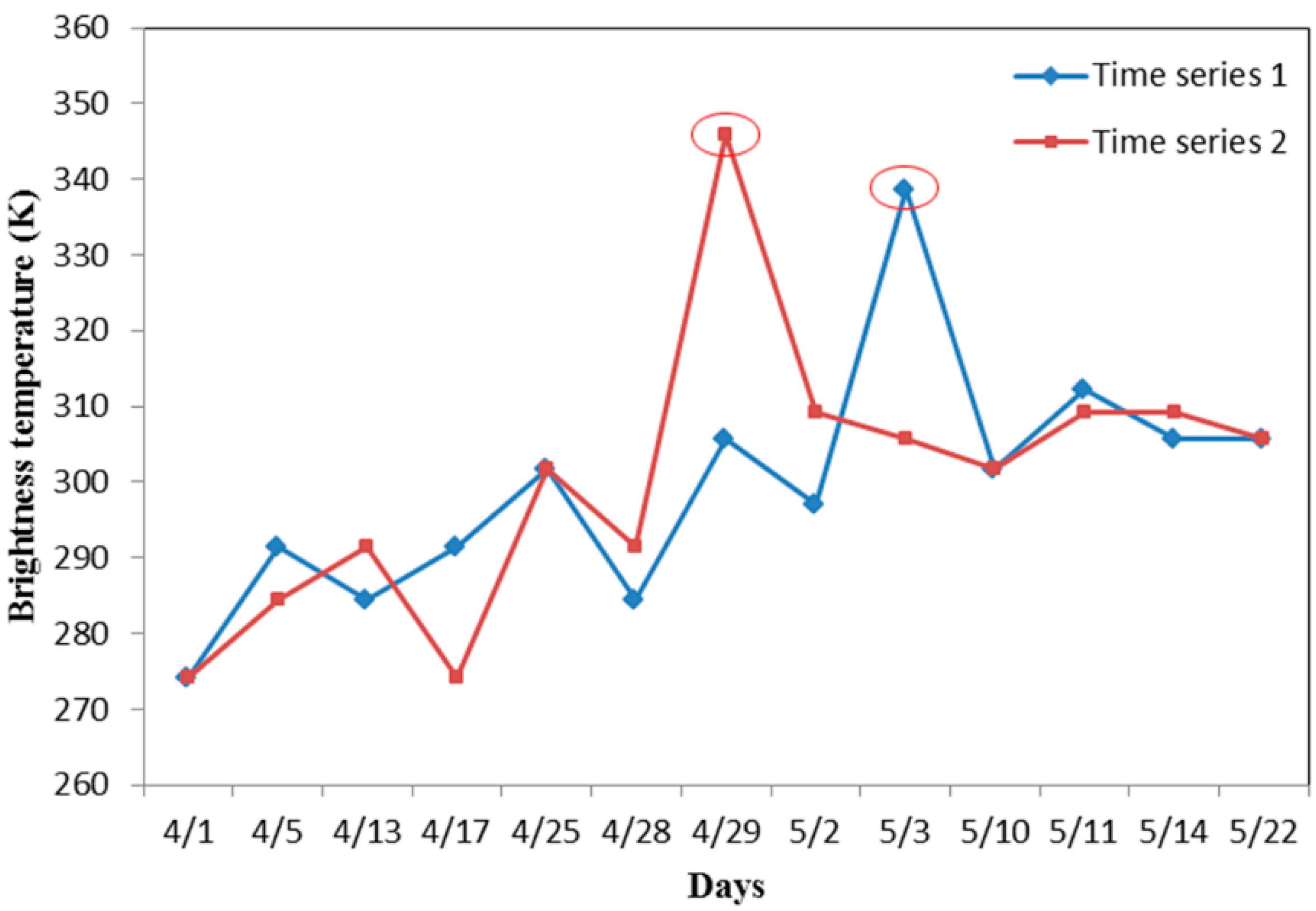
For single-date fire detection methods, a temperature anomaly is the variation between a particular temperature and the average temperature for its neighboring pixels (Equation (1)) because the fire produces a local increase in temperature above that of the neighboring pixels. However, it is hard to obtain enough valid neighboring pixels when there is a large fire, and the window size must be large enough for high-resolution images. For multi-temporal images, a pixel that has a BT significantly higher than the values in previous moments will also be regarded as a fire pixel (Figure 10). Therefore, to compare the inspected pixel’s BT with its previous BTs, we added additional temporal information to STM by assigning different weights to multi-temporal images (Equation (12)). In addition, the mean absolute deviation varied tempestuously in different images, which resulted in instability in the forest fire detection results. To obtain a more robust result, we also added different weights to the calculation of the mean absolute deviation (Equation (13)). In summary, the approach was based on a change detection scheme that detects signal anomalies by utilizing the spatio-temporal domain of the HJ-IRS data.

Figure 10.
Time series of fire pixels. The red marks represent fire points.
Relative Fire Pixel Judgment
In this study, we used the BT from band 7 and the difference in the BTs from band 7 and band 8 to detect the forest fire. The background BTs from band 7 and band 8 were predicted using Equation (11), and the absolute deviation was calculated using Equation (13). For a potential pixel to be classified as a true fire pixel, it should satisfy the following Equations:
where ; , and are the observed BTs from band 7 and band 8 for pixel in the image acquired at time , respectively; and are the weighted background BTs calculated using Equations (11) and (12), respectively; and are calculated using Equation (13) with mean absolute deviations of and , respectively; and and are learning parameters that can be calibrated to control the detection results. For comparison, we chose and , as defined in [24].
4. Results and Discussion
4.1. Goodness of Fit
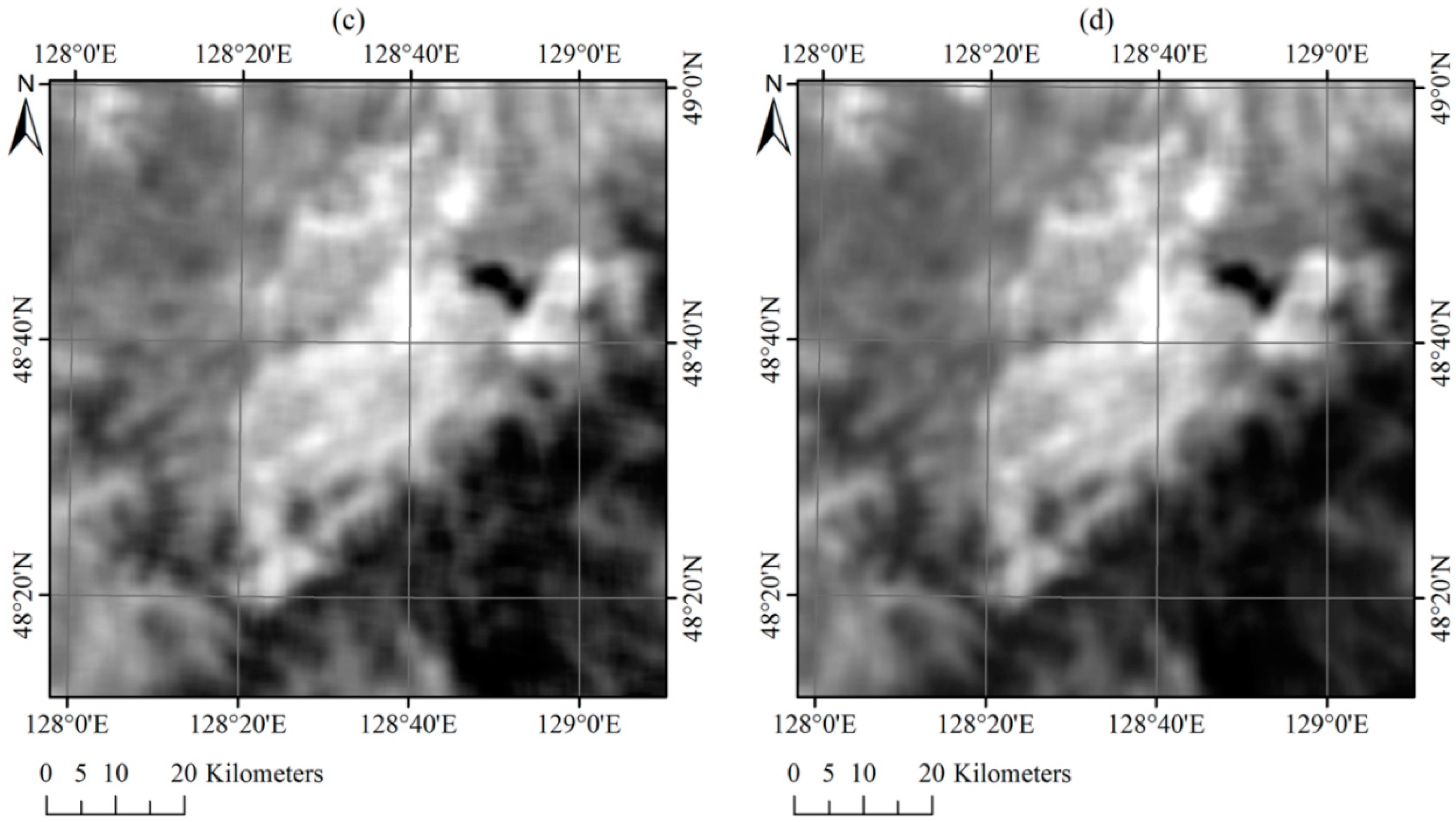
Figure 3 displays the images of the observed BTs from band 7 and band 8 on 22 May. We used these images to evaluate the quality of the background intensity predictions (goodness of fit). As mentioned previously (Section 3.2.4), we obtained the background values of the observed images using STM, which had been built using previous images. We first updated the spatial relationship using valid pixels in previous images. We then calculated the mean value as the background value of the inspected pixel using Equation (11). In this study, the size of the window was . For comparison, we obtained the background BTs of this image by averaging the neighboring pixels with the same window size. This processing can be regarded as an application of simple mean filtering. The predicted BT images are shown in Figure 11, which can be compared to the observed images in Figure 3.
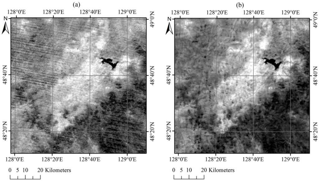

Figure 11.
BT images of band 7 (a) and band 8 (b) predicted using the spatio-temporal model (STM); and BT images of band 7 (c) and band 8 (d) predicted by averaging the neighboring pixels.
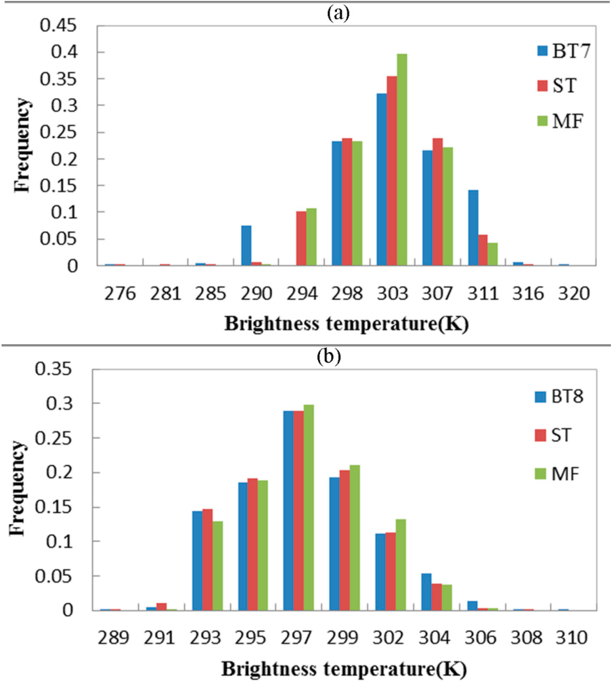
The HJ-IRS image acquired on 22 May was cloud free, and there was no fire in this image. Thus, the typical example image can be regarded as an actual background measurement. Figure 12 shows the frequency histograms of the background predictions and the actual background measurements from band 7 and band 8.

Figure 12.
Frequency histograms of the background BT predictions and the actual BTs measurements from band 7 (a) and band 8 (b). “BT” denotes the actual background BT measurements, “ST” denotes the background BTs predicted using STM, and “MF” denotes the background BTs predicted by averaging the neighboring pixels.
From Figure 11, it is obvious that the background BT images acquired using STM were closer to the real BT images than those obtained by averaging the neighboring pixels, which is adopted in the contextual algorithm. The histograms in Figure 12 also show that the distribution of the background BT images predicted by STM and the actual BT images were more consistent. More accurate background BT predictions lead to more satisfactory forest fire detection results. Therefore, the prediction process in the STM method is more suitable for forest fire detection. The method produced good prediction results primarily because the spatial relationship defined in STM eliminated the spatial heterogeneity between the inspected pixel and its valid neighboring pixels. In addition, the spatio-temporal model adapted to the multi-temporal remote sensing images because the spatial relationship was updated over time.
4.2. Accuracy of Forest Fire Detection
We applied the STM method and the contextual algorithm to the Yinanhe forest fire detection. The ground truth data discussed in Section 2.3 were used to evaluate the fire detection result. In the STM method, the size of window was 21 × 21. In our comparison, we used a series of contextual and absolute-threshold tests to detect the active fire pixels in every IRS image. The optimized selection of the valid neighbors and the window size was implemented as described in [24]. For the sake of comparison, the contextual algorithm used the same cloud masking method proposed in Section 3.2.2.
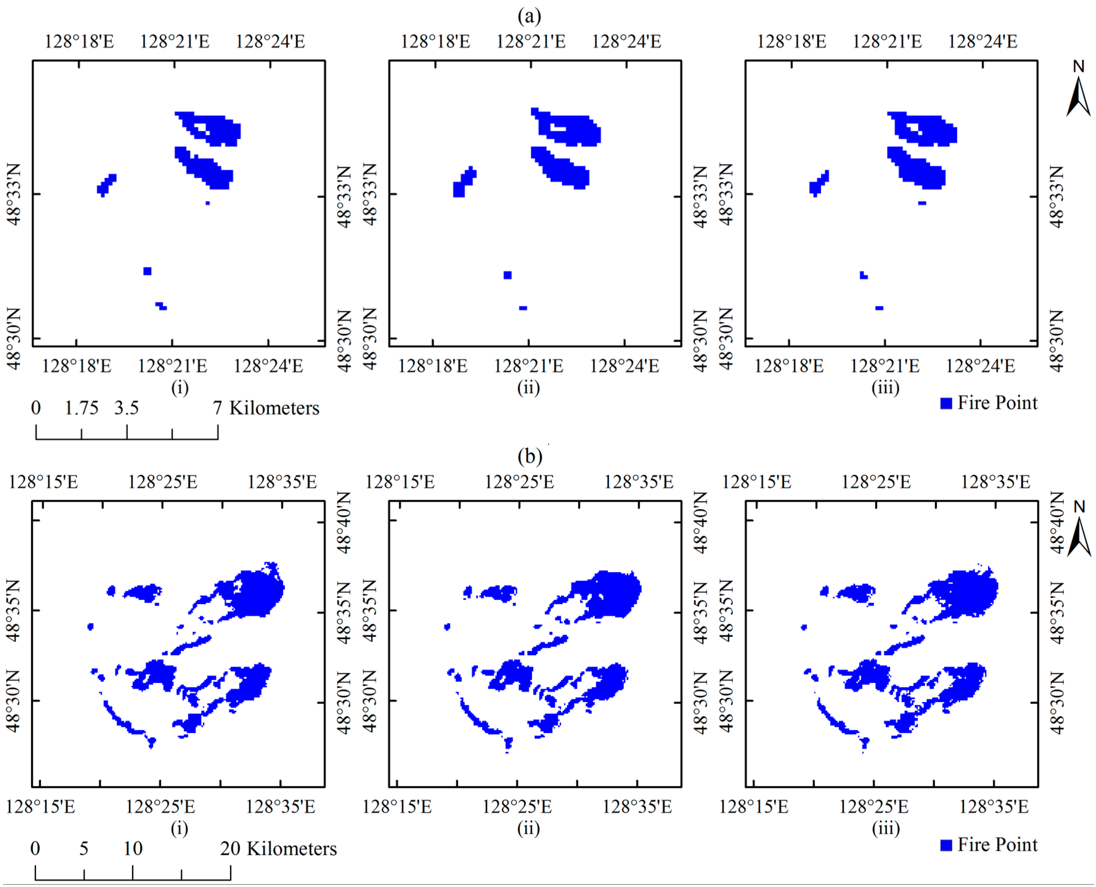
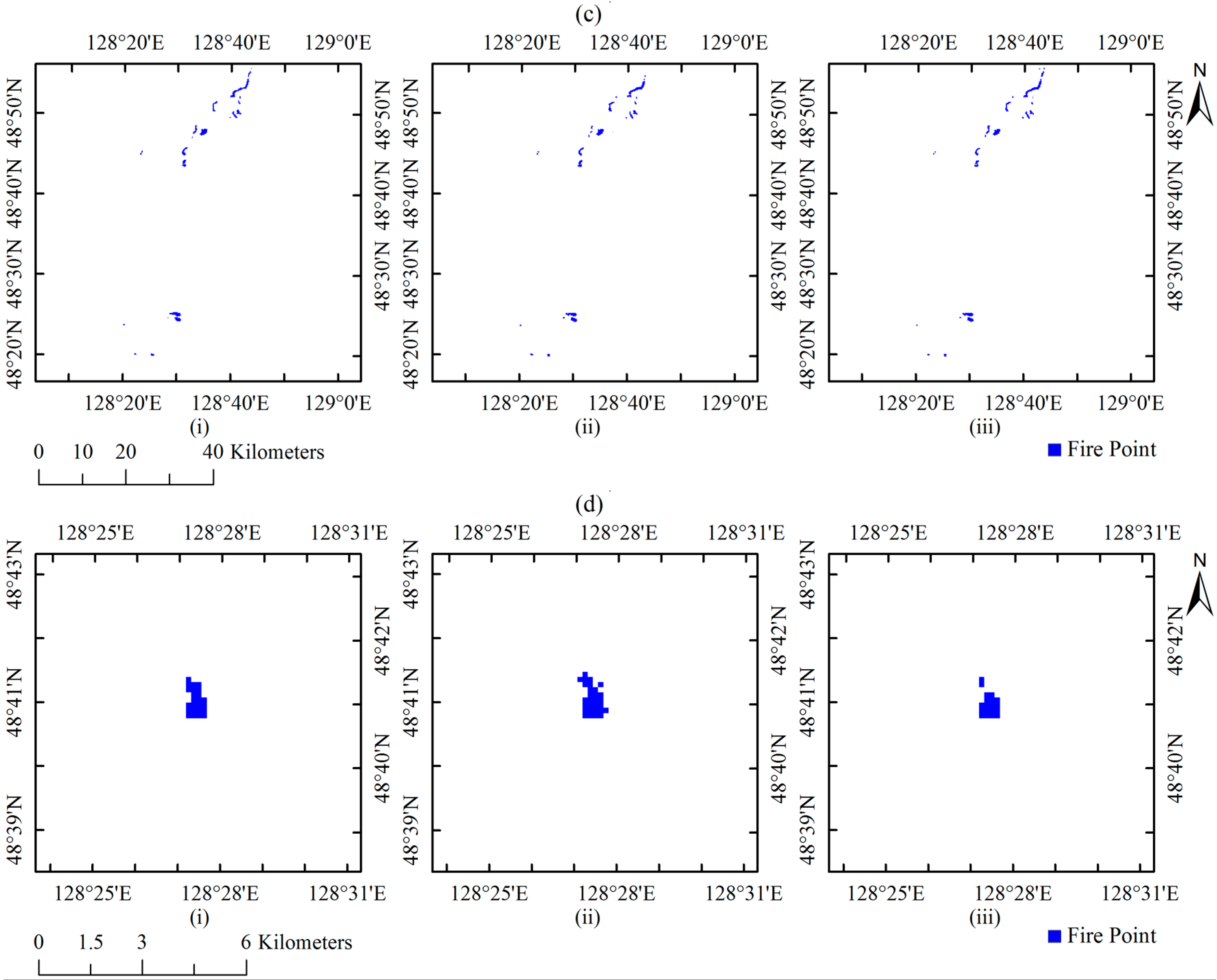
The maps (Figure 13) below show the STM method and contextual algorithm results. We used the ground truth data as references to compare the accuracies of the STM method results with those of the contextual algorithm results (Table 2). The commission errors and omission errors were calculated for each image.

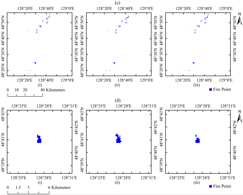
Figure 13.
Ground reference data (i) and forest fire detection results by contextual algorithm (ii) and STM (iii) for the days: 28 April 2009 (a); 29 April 2009 (b); 3 May 2009 (c); and 11 May 2009 (d).
Table 2.
Accuracies of the STM method and contextual algorithm results.
Herein, the commission error is the fraction of the wrongly detected fire pixels with regard to the extracted fire pixels, and the omission error is the fraction of fire pixels that were not detected with regard to the real fire pixels. The commission error is the inverse of the user’s accuracy, whereas the omission error is the inverse of the producer’s accuracy. According to Table 2, the STM method omission errors were obviously lower than those of the contextual algorithm. However, the STM method commission errors were slightly higher than those of the contextual method because the STM method detected more fire pixels. The overall omission error was 5.56%, which means that when the STM method was used, 3925 of 4158 fire pixels were correctly detected, at the same time, the overall commission error was 9.91%, which means that 399 “normal” pixels were wrongly detected as forest fire pixels. In reality, the detection result was satisfactory for the HJ-IRS data.
Taking into consideration the fitting quality and detection accuracy, the STM method as proposed in this study performed better than the contextual fire detection algorithm, which was confirmed in the Yinanhe forest fire detection example. As introduced in Section 3.2.4, the good detection results were primarily due to the following reasons: (i) a more accurate background intensity prediction; and (ii) the integration of the spatial contextual information and temporal information.
5. Strengths and Limitations of the STM Method
The STM method has some remarkable advantages. First, the background BT prediction is more accurate and robust than the contextual algorithm. The spatial heterogeneity has little effect on the forest fire detection result in STM. By using the STM, the algorithm is able to provide a satisfactory result in complex scenes. Second, the STM method takes full advantage of spatial contextual information and temporal information. The use of temporal information of the earth surface development is helpful for anomaly detection, which makes it possible for STM to detect more active fire pixels especially for small fire pixels.
Moreover, a powerful competitive advantage of the STM method is that the window size has little influence on the measurement accuracy, whereas the window size is crucial in contextual tests. When there is a large fire and the image has a high-resolution, such as that of the HJ-IRS data, a “cavity” often appears in the detection area (Figure 14) in contextual tests. The primary reason is that there are not a sufficient number of valid neighboring pixels to predict background intensities with a limited window size. In addition, larger window sizes often result in a larger amount of calculations and problems of spatial heterogeneity. In our contrast experiments, there was not a cavity in the contextual detection result because the contextual tests included an absolute fire pixel judgment, which eliminated the “cavity”.
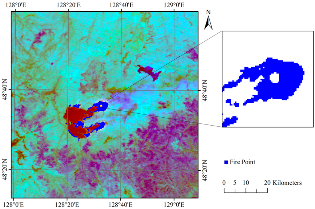
Figure 14.
The fire detection results using the contextual algorithm without the absolute fire pixel judgment produced a “cavity” in the detection area. The image was acquired on 29 April.
Regarding the spatio-temporal model, a potential fire pixel is regarded as a true fire pixel if the observed BT is higher than its neighboring pixels or its previous BTs. In other words, the relative fire pixel judgment is not only decided by the characteristics of the neighboring pixels but also by its previous characteristics. The integration of spatial contextual and temporal information allows the STM method to take full advantage of the two characteristics. In addition, background BTs calculated in the spatio-temporal domain are more robust, which can also mitigate the influence of the window size. Therefore, there were not “cavity” phenomena in the STM method results. A satisfactory result can be obtained using a small quantity of valid neighboring pixels in the STM method. This finding is verified in Figure 15. We can see that there is no positive connection between the number of fire pixels and the window size. Although the commission and omission errors decreased slowly with window size, small window sizes can lead to satisfactory results. In particular, we chose 21 × 21 as the optimal window size in this study because the omission error was smallest, and the commission error was acceptable when the window size was 21 × 21.
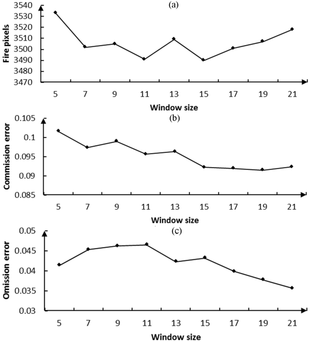
Figure 15.
Fire detection results of the image acquired on 29 April with different STM window sizes: (a) number of fire pixels; (b) commission error; and (c) omission error.
The STM method has two major limitations. (I) Historical images are required to initialize the model before the STM method is used for forest fire detection. If there are too many noisy pixels in the images, the modeling results could be unsatisfactory; (II) The remote sensing images used by the STM method should be acquired at approximately the same time of day. The comparison of multi-temporal images that are acquired at different times of day, especially for day and night, is meaningless.
6. Conclusions
A new forest fire detection approach based on STM has been described in this paper. The major novelties of this method lie in considering the correlations between the inspection pixel and its neighboring pixels and updating the spatial relationship defined in the model over time. STM can mitigate the adverse impacts of spatial heterogeneity on the prediction of background intensities by using the strong correlations between pixels. What is more, the integration of spatial contextual information and temporal information makes it a more robust model for anomaly detection.
To evaluate the performance of the proposed method, a case study was conducted to detect fire pixels in the Yinanhe forest. The results indicated that the STM method was capable of detecting forest fire pixels with a producer’s accuracy of 90.09% and a user’s accuracy of 94.45% when applied to HJ-IRS images. The STM method was also compared with the contextual algorithm. The comparison results suggested that the STM method performed better for background BT prediction and achieved comparable detection accuracies. In addition, the STM method was also more robust in terms of the selection of the window size.
However, the STM method was only tested during the fire season. Its performance throughout the year has not been verified. To improve the validation process, future work should be dedicated to conducting careful and quantitative validations of the STM method in different regions and seasons.
Acknowledgments
This work is jointly supported by the National Science and Technology Major Project (30-Y20A03-9003-15/16), the National Natural Science Foundation of China (Grant No. 41401474 and No. 41301393) and Young Scholars of Institute of Remote Sensing and Digital Earth, Chinese Academy of Sciences (Y5SJ1400CX).
Author Contributions
Lin Lei had the original idea for the study and wrote the original manuscript. Meng Yu and Yue Anzhi supervised the research and reviewed and edited the manuscript. Yuan Yuan and Liu Xiaoyi were responsible for the manuscript revisions. Chen Jingbo and Chen Jiansheng offered valuable comments on the manuscript. Zhang Mengmeng was responsible for the validation data collection and examination. All the authors read and approved the final manuscript.
Conflicts of Interest
The authors declare no conflict of interest.
Abbreviations
The following abbreviations are used in this manuscript:
| STM | Spatio-temporal model |
| MWIR | midwave infrared |
| LWIR | longwave infrared |
| NIR | near infrared |
| SWIR | shortwave infrared |
| BT | brightness temperature |
| SEVIRI | Spinning Enhanced Visible and Infrared Imager |
| DDM | Dynamic Detection Model |
| RST | robust satellite technique |
| ALICE | Absolute Local Index of Change of the Environment |
| MODIS | Moderate Resolution Imaging Spectroradiometer |
| CCD | charge-coupled device |
| IRS | infrared camera sensor |
| HJ-1 | Environment and Disaster Monitoring and Forecasting with a Small Satellite Constellation |
| LAADS | Level 1 and Atmosphere Archive and Distribution System |
| ROI | region-of-interest |
| DN | digital number |
References
- Loehman, R.A.; Reinhardt, E.; Riley, K.L. Wildland fire emissions, carbon, and climate: Seeing the forest and the trees—A cross-scale assessment of wildfire and carbon dynamics in fire-prone, forested ecosystems. For. Ecol. Manag. 2014, 317, 9–19. [Google Scholar] [CrossRef]
- Martell, D.L. A Review of recent forest and wildland fire management decision support systems research. Curr. For. Rep. 2015, 1, 128–137. [Google Scholar] [CrossRef]
- Wooster, M.J.; Xu, W.; Nightingale, T. Sentinel-3 SLSTR active fire detection and FRP product: Pre-launch algorithm development and performance evaluation using MODIS and ASTER datasets. Remote Sens. Environ. 2012, 120, 236–254. [Google Scholar] [CrossRef]
- He, L.; Li, Z. Enhancement of a fire detection algorithm by eliminating solar reflection in the mid-IR band: Application to AVHRR data. Int. J. Remote Sens. 2012, 33, 7047–7059. [Google Scholar] [CrossRef]
- Arino, O.; Casadio, S.; Serpe, D. Global night-time fire season timing and fire count trends using the ATSR instrument series. Remote Sens. Environ. 2012, 116, 226–238. [Google Scholar] [CrossRef]
- Hassini, A.; Benabdelouahed, F.; Benabadji, N. Active fire monitoring with level 1.5 MSG satellite images. Am. J. Appl. Sci. 2009, 6, 157. [Google Scholar] [CrossRef]
- Li, Z.; Nadon, S.; Cihlar, J. Satellite-based detection of Canadian boreal forest fires: Development and application of the algorithm. Int. J. Remote Sens. 2000, 21, 3057–3069. [Google Scholar] [CrossRef]
- Giglio, L.; Descloitres, J.; Justice, C.O. An enhanced contextual fire detection algorithm for MODIS. Remote Sens. Environ. 2003, 87, 273–282. [Google Scholar] [CrossRef]
- Amraoui, M.; DaCamara, C.C.; Pereira, J.M.C. Detection and monitoring of African vegetation fires using MSG-SEVIRI imagery. Remote Sens. Environ. 2010, 114, 1038–1052. [Google Scholar] [CrossRef]
- Csiszar, I.; Schroeder, W.; Giglio, L. Active fires from the Suomi NPP Visible Infrared Imaging Radiometer Suite: Product status and first evaluation results. J. Geophys. Res. Atmos. 2014, 119, 803–816. [Google Scholar] [CrossRef]
- Roberts, G.J.; Wooster, M.J. Fire detection and fire characterization over Africa using Meteosat SEVIRI. IEEE Trans. Geosci. Remote Sens. 2008, 46, 1200–1218. [Google Scholar] [CrossRef]
- Giglio, L.; Schroeder, W.; Justice, C.O. The collection 6 MODIS active fire detection algorithm and fire products. Remote Sens. Environ. 2016, 178, 31–41. [Google Scholar] [CrossRef]
- Laneve, G.; Castronuovo, M.M.; Cadau, E.G. Continuous monitoring of forest fires in the Mediterranean area using MSG. IEEE Trans. Geosci. Remote Sens. 2006, 44, 2761–2768. [Google Scholar] [CrossRef]
- Koltunov, A.; Ustin, S.L. Early fire detection using non-linear multitemporal prediction of thermal imagery. Remote Sens. Environ. 2007, 110, 18–28. [Google Scholar] [CrossRef]
- Mazzeo, G.; Marchese, F.; Filizzola, C. A Multi-temporal Robust Satellite Technique (RST) for forest fire detection. In Proceedings of the International Workshop on the Analysis of Multi-temporal Remote Sensing Images, Leuven, Belgium, 18–20 July 2007.
- Roberts, G.; Wooster, M.J. Development of a multi-temporal Kalman filter approach to geostationary active fire detection & fire radiative power (FRP) estimation. Remote Sens. Environ. 2014, 152, 392–412. [Google Scholar]
- China Centre for Resources Satellite Data and Application. Available online: http://www.cresda.com/CN/Satellite/3064.shtml (accessed on 21 March 2016).
- Zhang, Y.; Liu, Z.; Wang, Y. Inversion of aerosol optical depth based on the CCD and IRS sensors on the HJ-1 satellites. Remote Sens. 2014, 6, 8760–8778. [Google Scholar] [CrossRef]
- Wang, Q.; Wu, C.Q.; Li, Q. Chinese HJ-1A/B satellites and data characteristics. Sci. China Earth Sci. 2010, 53, 51–57. [Google Scholar] [CrossRef]
- Csiszar, I.; Morisette, J.T.; Giglio, L. Validation of active fire detection from moderate-resolution satellite sensors: The MODIS example in northern Eurasia. IEEE Trans. Geosci. Remote Sens. 2006, 44, 1757–1764. [Google Scholar] [CrossRef]
- Calle, A.; González-Alonso, F.; Merino De Miguel, S. Validation of active forest fires detected by MSG-SEVIRI by means of MODIS hot spots and AWiFS images. Int. J. Remote Sens. 2008, 29, 3407–3415. [Google Scholar] [CrossRef]
- Liew, S.C.; Shen, C.; Low, J. Validation of MODIS fire product over Sumatra and Borneo using high resolution SPOT imagery. In Proceedings of the 24th Asian Conference on Remote Sensing and 2003 International Symposium on Remote Sensing, Busan, South Korea, 9–13 October 2003.
- MODIS Policies. Available online: https://lpdaac.usgs.gov/user_services/modis_policies (accessed on 21 March 2016).
- Wang, S.D.; Miao, L.L.; Peng, G.X. An improved algorithm for forest fire detection using HJ data. Procedia Environ. Sci. 2012, 13, 140–150. [Google Scholar] [CrossRef]
- Yang, J.; Gong, P.; Zhou, J.X. Detection of the urban heat island in Beijing using HJ-1B satellite imagery. Sci. China Earth Sci. 2010, 53, 67–73. [Google Scholar] [CrossRef]
- Zhan, J.; Fan, C.; Li, T. A forest firespot automatic detection algorithm for HJ-IRS imagery. Geomat. Inf. Sci. Wuhan Univ. 2012, 37, 1321–1324. (In Chinese) [Google Scholar]


© 2016 by the authors; licensee MDPI, Basel, Switzerland. This article is an open access article distributed under the terms and conditions of the Creative Commons Attribution (CC-BY) license (http://creativecommons.org/licenses/by/4.0/).