Article

Variability and Changes in Climate, Phenology, and Gross Primary Production of an Alpine Wetland Ecosystem

1
Beijing Key Laboratory of Wetland Services and Restoration, Institute of Wetland Research, Chinese Academy of Forestry, Beijing 100091, China
2
Sichuan Zoige Wetland Ecosystem Research Station, Tibetan Autonomous Prefecture of Aba 624500, China
3
College of Life Sciences, University of Chinese Academy of Sciences, Beijing 100049, China
4
Chengdu Institute of Biology, Chinese Academy of Sciences, Chengdu 610041, China
5
Beijing Gardens Green Bureau, Beijing 100013, China
6
Key Laboratory of Adaptation and Evolution Plateau Biota, Northwest Institute of Plateau Biology, Chinese Academy of Science, Xining 810008, China
7
Department of Forest Ecology and Management, Swedish University of Agricultural Sciences, Umeå 90183, Sweden
8
Department of Microbiology and Plant Biology, Center for Spatial Analysis, University of Oklahoma, Norman, OK 73019, USA
9
Institute of Biodiversity Science, Fudan University, Shanghai 200433, China
*
Author to whom correspondence should be addressed.
These authors contributed equally to this work.
Remote Sens. 2016, 8(5), 391; https://doi.org/10.3390/rs8050391
Submission received: 10 December 2015 / Revised: 24 March 2016 / Accepted: 29 April 2016 / Published: 6 May 2016
(This article belongs to the Special Issue What can Remote Sensing Do for the Conservation of Wetlands?)

Abstract

:
Quantifying the variability and changes in phenology and gross primary production (GPP) of alpine wetlands in the Qinghai–Tibetan Plateau under climate change is essential for assessing carbon (C) balance dynamics at regional and global scales. In this study, in situ eddy covariance (EC) flux tower observations and remote sensing data were integrated with a modified, satellite-based vegetation photosynthesis model (VPM) to investigate the variability in climate change, phenology, and GPP of an alpine wetland ecosystem, located in Zoige, southwestern China. Two-year EC data and remote sensing vegetation indices showed that warmer temperatures corresponded to an earlier start date of the growing season, increased GPP, and ecosystem respiration, and hence increased the C sink strength of the alpine wetlands. Twelve-year long-term simulations (2000–2011) showed that: (1) there were significantly increasing trends for the mean annual enhanced vegetation index (EVI), land surface water index (LSWI), and growing season GPP (R2 ≥ 0.59, p < 0.01) at rates of 0.002, 0.11 year−1 and 16.32 g·C·m−2·year−1, respectively, which was in line with the observed warming trend (R2 = 0.54, p = 0.006); (2) the start and end of the vegetation growing season (SOS and EOS) experienced a continuous advancing trend at a rate of 1.61 days·year−1 and a delaying trend at a rate of 1.57 days·year−1 from 2000 to 2011 (p ≤ 0.04), respectively; and (3) with increasing temperature, the advanced SOS and delayed EOS prolonged the wetland’s phenological and photosynthetically active period and, thereby, increased wetland productivity by about 3.7–4.2 g·C·m−2·year−1 per day. Furthermore, our results indicated that warming and the extension of the growing season had positive effects on carbon uptake in this alpine wetland ecosystem.

Graphical Abstract

1. Introduction

Wetlands only cover 3%–8% of the Earth’s land surface, but store 15%–30% of the world’s terrestrial soil carbon [1,2], indicating that they play an important role in the global carbon (C) cycle and potentially have a significant impact on global climate change [3,4,5]. Vegetation phenology is a fundamental determinant affecting the processes of carbon, water, and energy exchange in wetland ecosystems [6,7]. Phenology determines the timing and duration of the photosynthetically active canopy and drives annual carbon uptake in wetland ecosystems [8,9,10]. However, changes in the global and regional climate, such as rising global mean temperatures and changing precipitation regimes [11,12,13], have significantly affected wetland vegetation dynamics and carbon dynamics. Warming may stimulate plant phenological development, increase nutrient mineralization rates, and lengthen the growing season, which in turn may increase plant primary production and carbon sequestration [14,15]. Furthermore, warming can accelerate biospheric metabolism, resulting in a greater release of greenhouse gases to the atmosphere, which in turn reinforces anthropogenic warming [3,16]. Therefore, quantifying the relationships among climate change, phenological variability, and vegetation production is crucial for investigating accurate C budgets in alpine wetland ecosystems, especially in the context of global warming.
The largest highland wetland in the world, the Zoige alpine wetland, is situated at the eastern edge of the Qinghai–Tibetan Plateau. Because of the high altitude, this wetland is highly sensitive to climatic changes [14,17,18]. Continuously rising temperatures and declining precipitation characterize climate change in this region [4,5]. These changes may have decreased soil moisture and accelerated thawing of permafrost, causing wetland degradation and potentially increasing CO2 efflux to the atmosphere. Climatic changes may also influence plant phenology, i.e., the timing of flowering and other developmental stages. Shifts in plant phenology can affect the carbon cycle, water cycle, and energy fluxes through photosynthesis and evapotranspiration, and potentially increase CO2 influx to the wetland ecosystem. Moreover, the changes in local climate may produce a positive feedback, mediated by the greenhouse effect from increased CO2 emissions [5]. Therefore, to improve our understanding of C balance dynamics in the Zoige alpine wetland, the effects of warming and phenological variability should be studied simultaneously.
Over the past few decades, development of the eddy covariance (EC) method and satellite-based models have greatly increased opportunities for exploring the potential effects of climate change and vegetation phenology on C exchange between terrestrial ecosystems and the atmosphere. The EC method can provide continuous measurements of ecosystem-level exchanges of carbon, water, and energy fluxes [19,20], but such measurements have only been made at several research sites and often over short time periods [21]. Remote sensing (RS) technology is an important tool in the characterization of vegetation phenology [22,23] and estimation of gross primary production (GPP) [24]. It has become an effective tool to estimate either GPP or net primary production (NPP) at regional scales, which can be compatible with the EC flux tower footprint [25,26]. Recently, a satellite-based, vegetation photosynthesis model (VPM) developed by Xiao et al. simulated GPP based on the conceptual partitioning of chlorophyll and non-photosynthetically active vegetation within the canopy. The VPM model has been further developed and has the potential to scale up in situ observations of GPP from EC flux tower sites across ecosystems [25,27,28,29]. However, performance of the VPM model in simulating the long-term GPP of alpine wetland ecosystems and application to investigation of the relationships among wetland phenology, vegetation production, and climate change is still unknown.
Therefore, the primary objectives of this study were to: (1) investigate the changes in GPP and land surface phenology, as delineated by observed CO2 fluxes and vegetation indices during 2008–2009; (2) examine the variability and changes in climate, vegetation phenology, and gross primary production of an alpine wetland ecosystem; and (3) investigate the links between phenological events and wetland carbon uptake. There are very few flux tower sites in alpine wetlands, and this evaluation does highlight the limitations of in situ flux data and the need to evaluate production efficiency models, including the VPM model. As such, this study will also improve our understanding of the mechanisms underlying the current trends of vegetation phenology and carbon budgets observed in alpine wetlands and further explore the potential of remote sensing for monitoring and investigating regional or global C budgets.

2. Materials and Methods

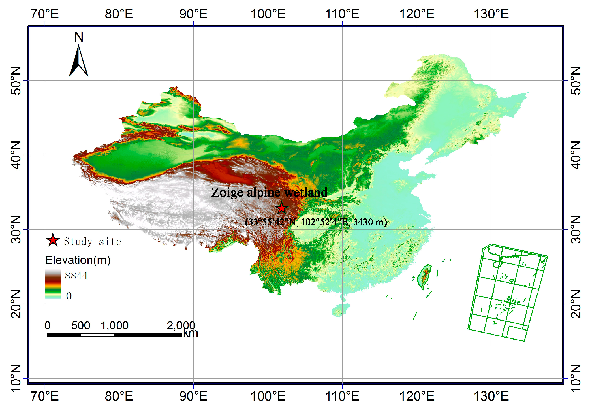
2.1. Site Description

Our study was carried out in an alpine wetland ecosystem of the National Wetland Natural Reserve of Zoige, located at the northeast edge of the Qinghai–Tibetan Plateau (33°55′42″N, 102°52′4″E). The alpine wetlands of this region cover an area of 6180 km2, which is 31.5% of the whole plateau of Zoige. The site has an average altitude of 3430 m above sea level (Figure 1). This region belongs to the cold Qinghai–Tibetan climatic zone. The climate of this region is characterized by a long period of frost (October to April) and a relatively short growing season (May to September). The mean annual air temperature in 2008 was 1.5 °C lower than the long-term (1990–2009) mean (1.6 °C); whereas the respective value in 2009 was 2.6 °C. The annual precipitation (rainfall and snowfall) in 2008 and 2009 was 465 and 596 mm, respectively, which is lower than the long-term mean (623 mm). There are two peaks of rainfall, in May and August. The air pressure is low, about 668.8 hPa, due to its high altitude.
The height of plants is about 50–80 cm. The dominant vegetation at the dry hummocks is composed of Kobresia tibetica, Cremanthodium pleurocaule, and Potentilla, accounting for approximately 45% of the site area. Carex muliensis (CM) and Eleocharis valleculosa (EV) are the two predominant plant species; they are scattered in hollow areas and cover 90% of the remaining aquatic surface. The size of CM and EV hollows is about 5 m2 on average, with 3 to 7 cm standing water. The size of dry hummocks (DH) is about 0.8 m2 and their height is from 20 to 50 cm. At regional scale, hollows account for a small part of the total area even in the growing season. In the non-growing season, both CM and EV sites were covered with ice. The total aboveground and belowground biomass is 166–184 and 2104–2246 g·m−2, respectively. The low temperature and large diurnal temperature variation inhibit the decomposition of plant litter and soil organic matter and stimulate the deposition of peat [5]. The depth of peat in the Zoige alpine wetland ranges from 0.3 to 8.8 m. In all sites, the greatest root density was found in the 0 to 20 cm soil depth. Below that layer there is a peat layer ranging from 50 to 80 cm in thickness. In the past several decades, artificial drainage for cultivation and peat mining greatly modified the water table, the ratio of hollows to hummocks, and the vegetation composition, leading to a potential change of GPP.

2.2. Datasets

Site-specific CO2 flux and climate data measurements were conducted by the EC flux tower, which was installed at a flat site in the alpine wetland in October 2007 to continuously measure the net ecosystem CO2 exchange (NEE) between the vegetation and atmosphere. The footprint of this flux tower is approximately 200–250 m. A three-axis sonic anemometer with a fast response open path infrared CO2/H2O gas analyzer (IRGA, LI 7500, LI-COR Inc., Lincoln, NE, USA) was installed at a height of 2.2 m above ground level to measure the fluctuations in three wind components (w, u, v) and CO2 fluxes. Data quality control was also implemented to reduce measurement-induced uncertainties. Daily GPP and NEE data during 2008–2009 were then used to analyze the dynamics of wetland phenology. The averaged eight-day GPP and climate data observed in 2008 and 2009 were utilized to support model simulations and validate the results of the VPM model. The daily weather dataset for the study site location was obtained from the climate database of the Zoige meteorological station (2000–2007, 2010–2011). The meteorological station is located about 15 km from the EC tower. More details on the instruments and the data quality control process are described in Hao et al. and Kang et al. [3,29].
Site-specific vegetation indices were derived from MODIS datasets. We downloaded the eight-day composite MOD09A1 datasets for the 2000–2011 period from the Oak Ridge National Laboratory’s Distributed Active Archive Center (DAAC) website [30]. Then, reflectance values of four spectral bands (blue (459–479 nm), red (620–670 nm), near infrared (NIR 841–876), and shortwave infrared (SWIR1628–1652) over 2000–2011 were used to calculate three vegetation indices: normalized difference vegetation index (NDVI), enhanced vegetation index (EVI), and land surface water index (LSWI) [27].
N D V I = ρ n i r ρ r e d ρ n i r + ρ r e d
E V I = G × ρ n i r ρ r e d ρ n i r + ( C 1 × ρ r e d C 2 × ρ b l u e ) + L
L S W I = ρ n i r ρ s w i r ρ n i r + ρ s w i r
where G = 2.5, C1 = 6, C2 =7.5, L = 1, and ρnir, ρred, ρblue, and ρswir are the reflectance of NIR, red, blue, and SWIR bands, respectively [23,27,29,31,32].
The three vegetation indices calculated from surface reflectance were affected by noise from clouds and cloud shadows [23]. Therefore, we used a simple gap filling method to gap-fill vegetation index values for which cloudy pixels existed in the time series [31]. Based on the two-step gap-filling procedure reported in earlier studies [31], we first selected a three-point time-series filter (X(t − 1), X(t), and X(t + 1)) and used values of non-cloudy pixels in this window to replace cloudy pixels. If both the X(t − 1) and X(t + 1) pixels were reliable and X(t) was unreliable, the average value of X(t − 1) and X(t + 1) was used to replace X(t). If only one pixel (either X(t − 1) or X(t + 1)) was cloud-free and reliable and X(t) was unreliable, we used that pixel value to replace X(t). If the algorithm did not result in a three-point time series filter, we then extended it to a five-point time series filter, X(t − 2), X(t − 1), X(t), X(t + 1), X(t + 2), using the same procedure as the above three-point time series filter [31].
Earlier studies have indicated that time series of greenness-related GPP, vegetation indices (e.g., NDVI, EVI), and water-related vegetation indices (LSWI) can be used to identify the green-up phase (from the beginning of leaf budding to the completion of full leaf expansion) and the senescence/leaf-drop phase at the canopy level [31,33]. In this study, GPP, NDVI, EVI, and LSWI threshold values (GPP ≥ 1 g·C·m−2·day−1, NDVI ≥ 0.3, EVI ≥ 0.2, LSWI ≥ −0.1) were used to delineate vegetation phenology [25,26,34].
The above three vegetation indices calculated from the reflectance of spectral bands have been proven to effectively monitor vegetation phenology. Furthermore, the time series of NDVI, EVI, and LSWI provided valuable insight into the processes (e.g., growing season length and water condition) that regulate ecosystem carbon exchange. Therefore, it is important to select these vegetation indices and to evaluate their biophysical and phenological performance in wetland ecosystems for more accurate GPP prediction.

2.3. The Satellite-Based Vegetation Photosynthesis Model

Based on the conceptual partitioning of chlorophyll and non-photosynthetically active vegetation (NPV) within a canopy, Xiao et al. developed the vegetation photosynthesis model (VPM) for estimation of GPP using the following function [27]:
G P P = ε g × F P A R chl × P A R
where FPARchl is the fraction of PAR absorbed by chlorophyll in the canopy, εg is the light use efficiency (μmol CO2/μmol photosynthetic photon flux density, PPFD), and PAR is the photosynthetically active radiation (μmol PPFD). FPARchl and εg are estimated as follows [25,26,29]:
F P A R chl = α × E V I
ε g = ε 0 × T scalar × W scalar × P scalar
T s c a l a r = ( T T min ) ( T T max ) [ ( T T min ) ( T T max ) ] ( T T o p t ) 2
W s c a l a r = 1 + L S W I 1 + L S W I max
P s c a l a r = 1 + L S W I 2
where ε0 is the maximum light use efficiency (LUE) (μmol CO2/μmol PPFD), and Tscalar, Wscalar, and Pscalar are the downregulation scalars for the effects of temperature, water, and leaf phenology on LUE, respectively. Tmin, Tmax, and Topt are the minimum, maximum, and optimal temperature for photosynthetic activities, respectively. LSWImax is the maximum LSWI (land surface water index) over the study period.
In the VPM model, ε0 is estimated for each type of ecosystem individually. In order to obtain the ε0 values for the alpine wetland, we estimated the nonlinear model between observed NEE and PAR by using the Michaelis–Menten function (Equation (10)), based on data collected during the peak period of vegetation growth in 2008 and 2009. Here, we used 0.53 μmol CO2/μmol PPFD as ε0 for 2008 and 2009:
N E E = ε 0 × P A R × G P P max ε 0 × P A R + G P P max R e c o
where the GPPmax (mg CO2 m−2·s−1) is the ecosystem maximum photosynthetic capacity and Reco is ecosystem respiration. The estimated ε0 value is used as an estimate of the maximum light use efficiency parameter in the VPM model.
In the calculation of Tscalar [27], Tmin, Topt, and Tmax values vary among vegetation types. For the alpine wetland ecosystem in our study, when air temperature falls below Tmin, Tscalar is set to zero. We used Tmin of 0 °C, Topt of 16 °C, and Tmax of 32 °C, based on the relationship between temperature and photosynthesis over 2008–2009.
Estimation of site-specific LSWImax is dependent on the time series of remote sensing data. As a parameter describing water status, LSWImax varies across years. The maximum LSWI value within the plant-growing season was selected as an estimate of LSWImax [25,27,31]. Based on the analysis of LSWI seasonal dynamics derived from MODIS image data from 2008 to 2009, the LSWImax value was 0.26 and 0.36 for 2008 and 2009, respectively.
More details on parameters and functions of the validated VPM model are described in Kang et al. [29]. By running the VPM model at an eight-day time scale with the validated parameters, vegetation indices derived from the eight-day MODIS surface reflectance product, and site-specific data of air temperature and PAR during 2000–2011, we obtained the GPP data for each year.

2.4. Model Validation

The VPM model was run for the same two years to produce the corresponding GPP data. The observed and modeled GPP results for both 2008 and 2009 were compared to check VPM’s applicability for the Zoige alpine wetland. To analyze the correspondence between the simulated and observed results, we adopted three statistical criteria for the validation tests: the coefficient of determination (R2), the root of mean square error (RMSE), and the relative mean deviation (RMD). Each criterion investigates a specific aspect of the correlation.
Seasonal patterns of GPP from this ecosystem for the observed and VPM modeled outputs were validated by Kang et al. [29]. Comparisons between the simulated and observed eight-day GPP fluxes indicated that the VPM model captured the seasonal variations of observed GPP for the simulated two years reasonably well. The model creditably captured the U pattern of the plant growth driven by the temperature variation. In addition, the linear regression analysis of the modeled and observed GPP showed a general clustering of the data along an approximate 1:1 line with a strong correlation (R2 = 0.77, p < 0.0001). The RMSE and RMD values were 9.74% and −10.67%, respectively. In general, by comparing the modeling results with the observations, we gained confidence in the applicability of the VPM model for this alpine wetland ecosystem. We then upscaled the VPM model to examine the long-term variability and changes in climate, vegetation phenology, and gross primary production for the Zoige alpine wetland over the 2000–2011 period. By running the VPM model for this 12-year baseline climate scenario, we obtained seasonal and annual EVI, LSWI, GPP, and land surface phenology dynamics for each year.

3. Results

3.1. Land Surface Phenology as Delineated by Observed CO2 Fluxes and Vegetation Indices

Table 1 summarizes the land surface phenology, i.e., the start and end dates of the growing season (SOS and EOS), as delineated by the estimated GPP (GPPEC) data from the EC flux tower and MODIS-based vegetation indices (NDVI, EVI, and LSWI). The leaf-on and leaf-off phases of the Zoige wetlands delineated by seasonal GPP started in about April and October, respectively. Compared with GPPEC, EVI and LSWI have the potential to more accurately identify the SOS and EOS in the Zoige wetland. LSWI also appeared to offer a more accurate alternative approach to delineate the SOS and EOS than EVI (Table 1). Furthermore, the land surface phenology defined by GPPEC and LSWI indicated that the SOS in 2009 was eight days earlier than in 2008, which could be attributed to the warmer and wetter climate conditions in 2009.

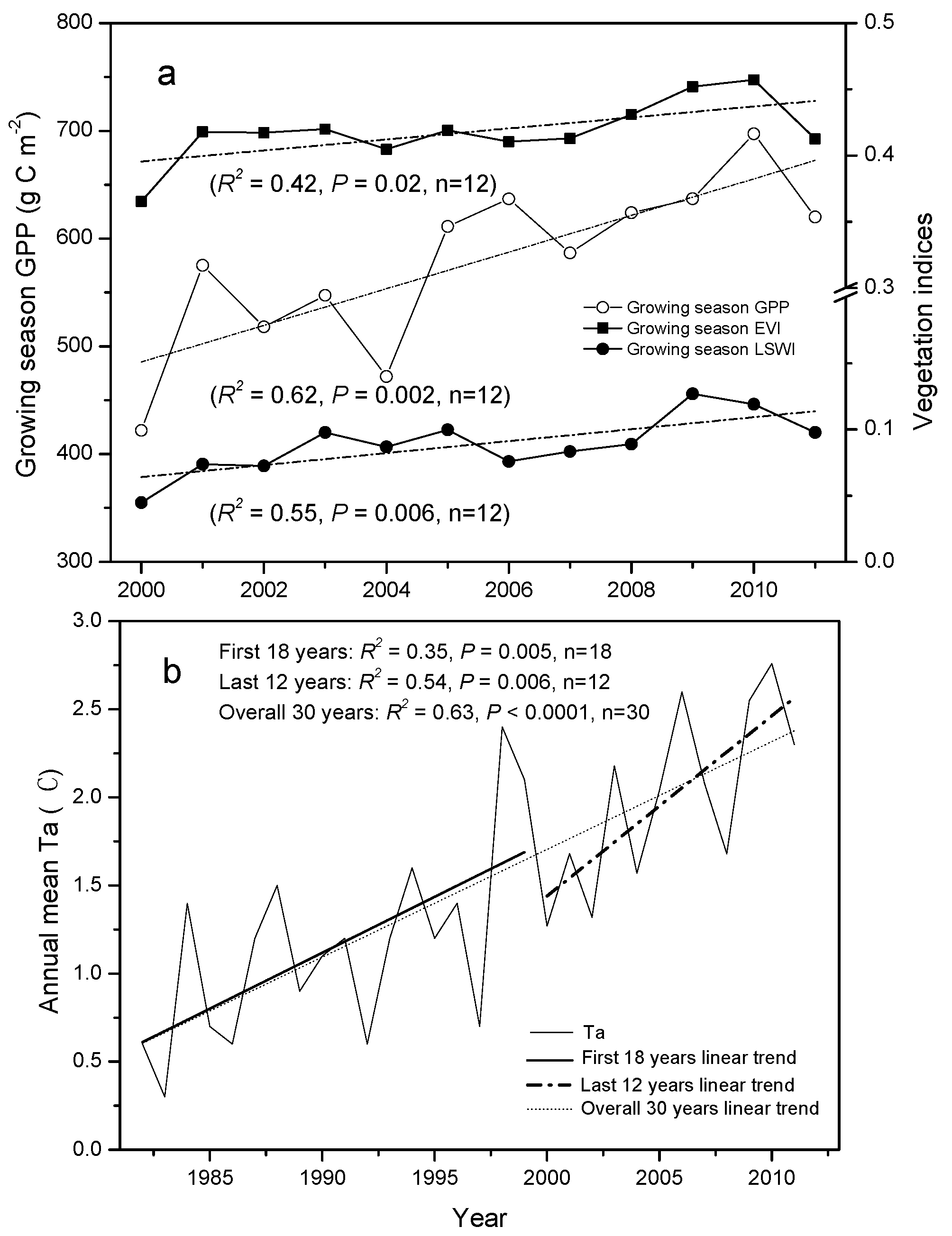
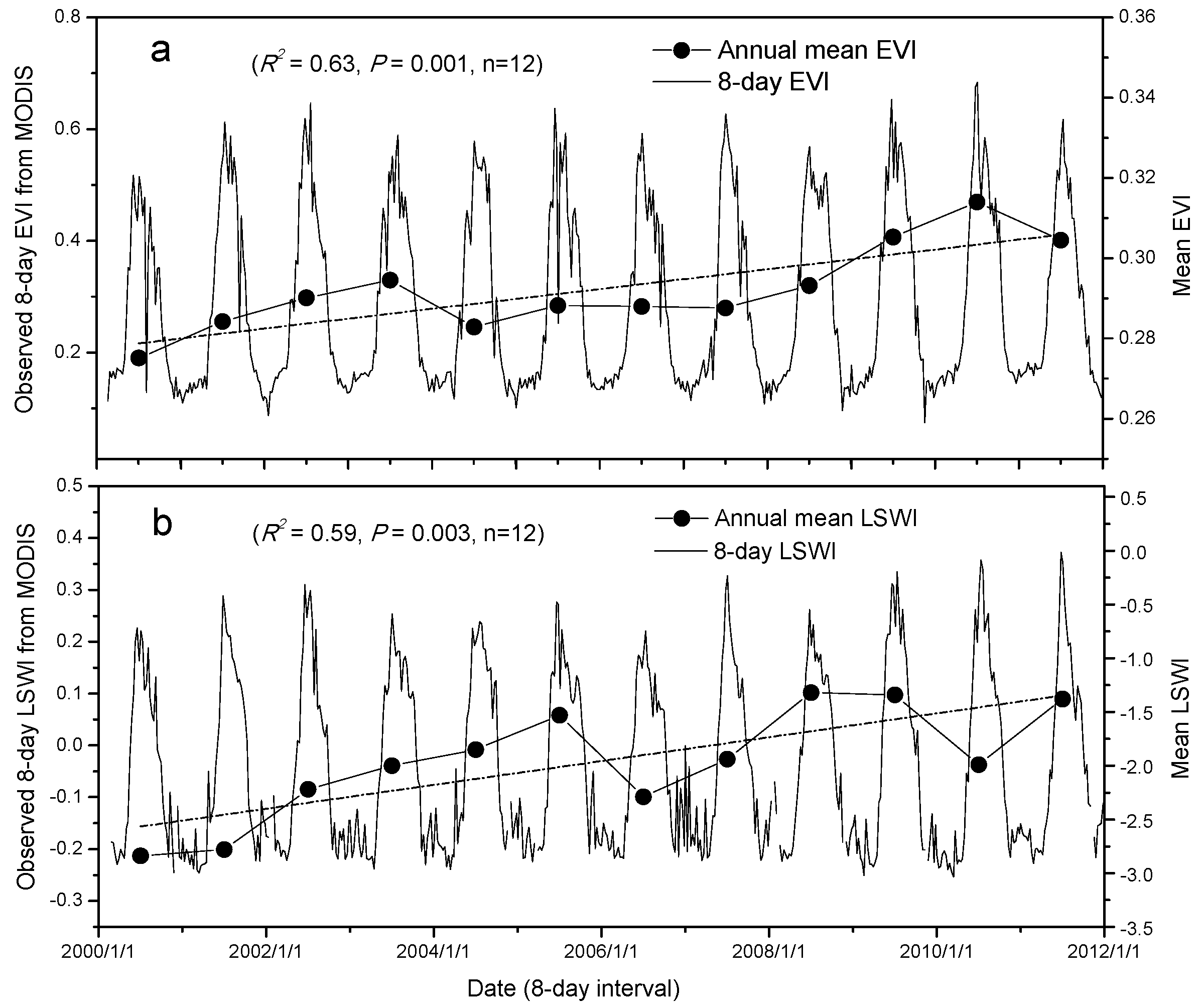
3.2. Trends in Vegetation Indices and GPP

We detected significantly increasing trends, with rates of 0.002 and 0.11 year−1, for annual mean EVI and LSWI, respectively, over the 2000–2011 period (Figure 2). The inter-annual variations in averaged EVI, LSWI, and GPP within the plant growing season also showed similar significantly increasing trends during the same period (R2 ≥ 0.42, p < 0.02), at rates of 0.004, 0.005 year−1, and 16.32 g·C·m−2·year−1, respectively (Figure 3a). Correspondingly, we found that the mean annual air temperature at the study site increased by 0.06, 0.07, and 0.12 °C·year−1 during the overall 30-year, first 18-year, and last 12-year periods, respectively (Figure 3b). There were strong and positive linear relationships between annual mean air temperature and vegetation indices (R = 0.72, p = 0.005) and GPP (R = 0.83, p < 0.0001). Warming explained 52% of the variation in vegetation indices and 69% of the variation in GPP. Regression analysis showed that the warming trend of mean annual air temperature triggered an increasing trend of 0.01 °C−1 for EVI, 0.41 °C−1 for LSWI, and 128.45 g·C·m−2·year−1·°C−1 for GPP, respectively (Figure 2 and Figure 3).

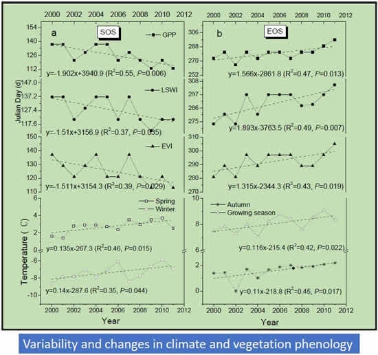
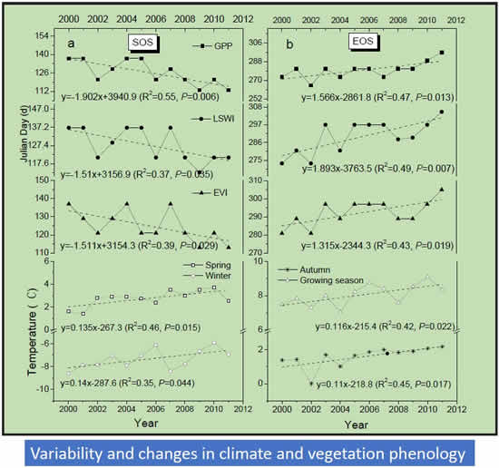
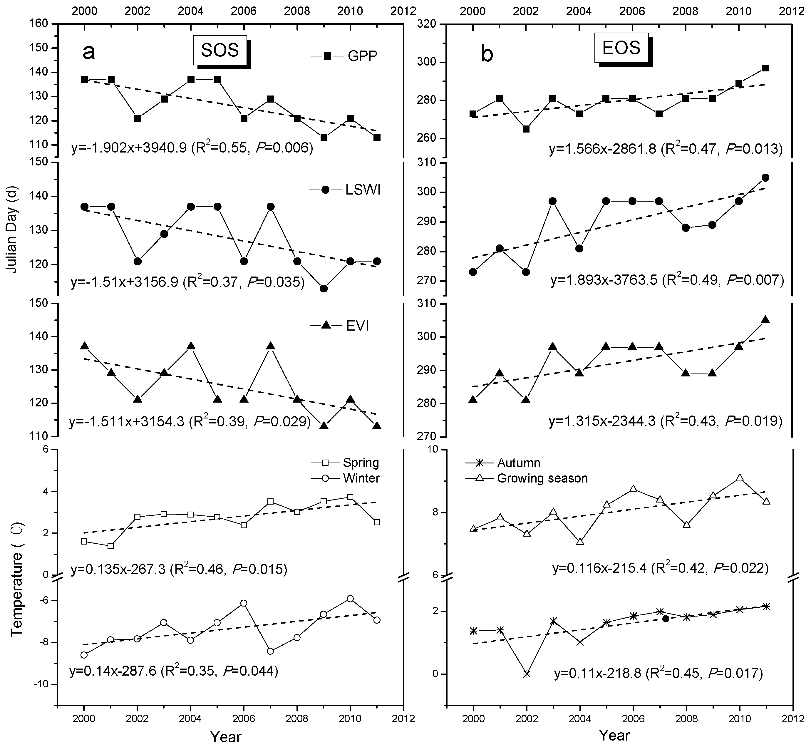
3.3. Trends in Vegetation Phenology (SOS and EOS)

We further examined the SOS and EOS trends of the Zoige wetland vegetation from 2000 to 2011 (Figure 4). The SOS results delineated by the EVI, LSWI, and GPP showed that there was a significant advancement of SOS at an average rate of 1.61 days·year−1 (R2 ≥ 0.37, p ≤ 0.035, n = 12). The earlier start of the growing season corresponded with similar increasing trends in the spring (R2 = 0.46, p = 0.015) and winter temperatures (R2 = 0.35, p = 0.044) during 2000–2011 (Figure 4a). We also ran a statistical analysis for the spring temperature, winter temperature, and SOS results delineated by the GPP, EVI, and LSWI. The results showed that there were negative relationships between the spring temperature and SOS, although these relationships were not significant (p > 0.05).
The EOS results delineated by the EVI, LSWI, and GPP showed that there was a clear delay for EOS at an average rate of 1.57 days·year−1 (R2 ≥ 0.41, p ≤ 0.03) (Figure 4b). This autumn phenology trend corresponded with a significant increase in autumn and growing season temperatures (p < 0.05). The mean temperature in autumn and growing season increased by about 0.11 (p = 0.017) and 0.12 °C·year−1 (p = 0.022) during 2000–2011, respectively. Overall, the advancement in SOS and delay in EOS extended the length of the growing season (LOS) by an average of 3.1 days·year−1 (p < 0.05).

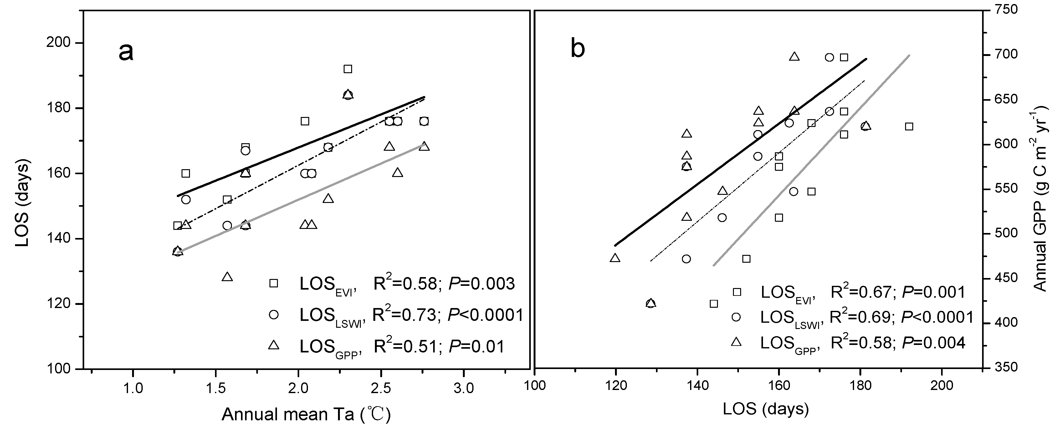
3.4. Correlation between Climate Change, Growing Season Length, and GPP

In order to further evaluate the relationship between temporal changes in annual mean air temperature (Ta), LOS, and GPP, we ran a series of correlation analyses. Clearly, there was a significantly positive relationship (R ≥ 0.71, p ≤ 0.01) between Ta and LOS (Figure 5a). Regression analysis between LOS and the annual C fluxes of GPP showed that LOS was closely and positively correlated with annual GPP (R ≥ 0.76, p ≤ 0.01), indicating that the growing season extension will cause an increase in GPP of 4.2 and 3.7 g·C·m−2·year−1 per day according to the LOS delineated by LSWI and GPP, respectively (Figure 5b). Furthermore, multiple regression analyses combining GPP, air temperature, and the growing season length were applied to evaluate their relative importance to GPP. Comparison of the standardized regression coefficients showed that the effects of warming on GPP were slightly stronger than those induced by the changed phenology (Table 2).

4. Discussion

Different vegetation indices vary in their phenological performance and can provide different insights into the processes (e.g., growing season length and water conditions) that regulate ecosystem carbon exchange [35]. Time-series NDVI data from remote sensing have been widely used for studying vegetation phenology at regional, landscape, and global scales, and a number of studies used a NDVI threshold value [30,36,37,38]. However, so far, few studies have evaluated the radiometric and biophysical performance of other vegetation indices, such as the EVI and LSWI from MODIS data. In this study, we used both an ecosystem-physiology approach and a remote sensing method to delineate the vegetation phenology of an alpine wetland ecosystem, and evaluated the phenology delineation performance of vegetation indices (NDVI, EVI, and LSWI) in relation to GPP. Our results clearly demonstrated that both EVI and LSWI more accurately identified the start and ending dates of plant growing season in the Zoige wetland, and hence had more biological and phenological significance in GPP predictions than the NDVI. Both EVI and LSWI provide new and complementary data to delineate land surface phenology, and these indices are more consistent with the CO2 flux data than the NDVI [39]. Moreover, LSWI was more stable than NDVI and EVI for delineating the vegetation phenology of alpine wetlands (Table 1), which is consistent with recent findings from savanna ecosystems [23]. LSWI is calculated as the normalized ratio between NIR and SWIR bands [33]. The combination of NIR and SWIR bands has the potential to retrieve leaf and canopy water content (equivalent water thickness, EWT, g·cm−2) and to more accurately delineate vegetation phenology [39]. The LSWI threshold value (≥−0.1) has been used to determine the emergence (leaf-on) and harvest (leaf-off) of croplands [24,34] and savanna woodlands [23].
Global climate change, especially warming, has already affected the timing of plant phenological events [40]. In this study, both the 12-year MODIS-based vegetation indices and model simulation results indicated that when the climate became warmer, the SOS advanced and the EOS delayed, which lengthened the growing season of the Zoige alpine wetland. Hence, plants interact with the seasonality of their environments, and changes in plant phenology can be regarded as sensitive indicators of climatic change [41]. A number of studies have shown that the growing season has significantly lengthened during the past decades under warmer conditions [36,37,38], but the connections and interactions between phenological variability and wetland C cycling are far from clear. An important finding in our study was that the recent lengthening of the growing season, as driven by warmer temperatures, can strongly enhance plant growth and increase wetland productivity at rates of 4.2 and 3.7 g·C·m−2·year−1 per day according to the LOS delineated by LSWI and GPP, respectively. Our results, however, are lower than the ORCHIDEE model average estimates of 5.8 g·C·m−2·year−1 across the Northern Hemisphere (>25°N) during 1980–2002 [37].
There is little doubt that a large number of environmental factors affect plant productivity; the real question is how much each of the main factors contributes to the observed signals [37]. Several studies have suggested that global warming is a key driving force for the observed increase in vegetation productivity at middle- and high-latitude ecosystems [42,43,44,45]. Indeed, we showed that the annual dynamics of vegetation indices and GPP were mainly driven by inter-annual variation in air temperature in the Zoige wetland. Generally, the warming signal can influence productivity through two pathways [46]. First, rising temperatures have a direct impact on plant photosynthesis and growth. Second, the lengthening of the growing season [47], changing plant phenology [48], stimulation of plant growth [46], increasing nutrient mineralization rates [49], reductions in soil water content [50], and alterations in plant species composition and community structure [44,51] have indirect impacts on productivity. In order to further evaluate the relative importance of changes in air temperature versus phenology in controlling GPP, we ran multiple regressions combining air temperature and the growing season length, delineated by EVI, LSWI, and GPP. Results from these regressions indicated that the effect of phenological shifts on GPP were slightly weaker than those induced by warming (Table 2). Further studies on the links between wetland carbon uptake and emissions and the many environmental drivers are needed in the future.
The net ecosystem C exchange is the balance between gross primary productivity and ecosystem respiration. In addition to GPP, ecosystem respiration is also sensitive to warming and changes in phenology [37,52]. Warmer air and soil temperatures will have direct effects on plant autotrophic and soil heterotrophic respiration. Previous studies have shown that warmer soil temperatures generally stimulate soil microbial activity, resulting in increased ecosystem respiration [53]. Generally, the balance of GPP (C influx) and ecosystem respiration (C efflux) determines whether terrestrial ecosystems will act as a net C sink or source under global climate changes [15,38]. In this study, however, we only focused on the effects of warming and the growing season extension on wetland C influx. As such, future studies on the C balance of the Zoige wetland should integrate continuous EC measurements and data from remote sensing over longer time periods with ecological modeling to evaluate whether warming will increase C emissions and if increased emissions will exceed the increases in C uptake.
Although we showed that remote sensing satellite observation has the capability to retrieve vegetation with relatively high precision and the VPM model can accurately capture the U pattern of the plant growth driven by variation in temperature and PAR in the alpine wetland, there still exist model uncertainty and some differences between simulated and observed GPP. The discrepancies may be attributed to three influencing factors on the modeling results. One is the sensitivity of the VPM model to PAR and temperature. The second factor is the remaining effect of angular geometry on surface reflectance and vegetation indices. The third factor is the error (overestimation or underestimation) of the observed GPP. More details of model uncertainty are described by Kang et al. [29].

5. Conclusions

In summary, our study showed that the land surface phenology of the Zoige alpine wetland, as described by the satellite vegetation indices, in particular the water-related vegetation indices (e.g., LSWI), corresponds well with the phenological patterns based on ecosystem physiology, as measured by the eddy covariance method. Further, long-term simulations (2000–2011) indicated increasing trends for annual mean EVI, LSWI, and annual GPP, respectively, which is in line with the observed warming trend. In addition, there were significant positive correlations between annual GPP and temperature and phenological period. Our results also show that when the climate became warmer, the SOS advanced and the EOS delayed, which resulted in prolongation of the wetland phenological period and, consequently, increases in vegetation productivity. The advanced SOS and delayed EOS phenology trends correspond with the increasing trends in seasonal and growing season temperatures. Furthermore, our results suggest that warming and extension of the growing season had positive effects on C uptake in this alpine wetland. The findings of our study have important implications for remote sensing analyses of wetland phenology and C cycling and for future simulation scenarios of vegetation growth and C budgets. Finally, further evaluation of VPM simulations for other wetlands is necessary before we can apply the model for regional, continental, and global simulations.

Acknowledgments

This work was supported by a National Nonprofit Institute Research Grant from CAFINT (Grant No. CAFINT2014K06), the National Youth Science Foundation of China (Grant No. 31300417), the National Natural Science Foundation of China (Grant No. 31170459), Si Chuan Province Youth Scientific and technological innovation research team (Grant No. 2015TD0026), and the NASA Earth Observing System (EOS) Data Analysis Program (Grant No. NNX09AE93G). We thank the principal investigators of the MODIS data products as well as the Oak Ridge National Laboratory’s (ORNL) Distributed Active Archive Center (DAAC) and the Earth Observing System (EOS) Data Gateway for making these MODIS products available. We thank the anonymous reviewers and editors for their valuable comments and suggestions on the earlier versions of the manuscript.

Author Contributions

All authors contributed to designing the study, developing the overall concept of data analysis, the preparation of figures and tables, and the revision of the manuscript.

Conflicts of Interest

The authors declare no conflict of interest.

References

  1. Turunen, J.; Tomppo, E.; Tolonen, K.; Reinikainen, A. Estimating carbon accumulation rates of undrained mires in Finland–application to boreal and subarctic regions. Holocene 2002, 12, 69–80. [Google Scholar] [CrossRef]
  2. Limpens, J.; Berendse, F.; Blodau, C.; Canadell, J.G.; Freeman, C.; Holden, J.; Roulet, N.; Rydin, H.; Schaepman-Strub, G. Peatlands and the carbon cycle: From local processes to global implications—A synthesis. Biogeosci. Discuss. 2008, 5, 1379–1419. [Google Scholar] [CrossRef]
  3. Hao, Y.B.; Cui, X.Y.; Wang, Y.F.; Mei, X.R.; Kang, X.M.; Wu, N.; Luo, P.; Zhu, D. Predominance of precipitation and temperature controls on ecosystem CO2 exchange in Zoige alpine wetlands of Southwest China. Wetlands 2011, 31, 413–422. [Google Scholar] [CrossRef]
  4. Chen, H.; Wu, N.; Gao, Y.H.; Wang, Y.F.; Luo, P.; Tian, J.Q. Spatial variations on methane emissions from Zoige alpine wetlands of Southwest China. Sci. Total Environ. 2009, 407, 1097–1104. [Google Scholar] [CrossRef] [PubMed]
  5. Chen, H.; Wu, N.; Wang, Y.; Zhu, D.; Yang, G.; Gao, Y.; Fang, X.; Wang, X.; Peng, C. Inter-Annual variations of methane emission from an open fen on the Qinghai-Tibetan Plateau: A three-year Study. PLoS ONE 2013, 8, e53878. [Google Scholar] [CrossRef] [PubMed]
  6. Zhao, M.F.; Peng, C.H.; Xiang, W.H.; Deng, X.W.; Tian, D.L.; Zhou, X.L.; Yu, G.R.; He, H.L.; Zhao, Z.H. Plant phenological modeling and its application in global climate change research: Overview and future challenges. Environ. Rev. 2013, 21, 1–14. [Google Scholar] [CrossRef]
  7. Wang, C.; Cao, R.Y.; Chen, J.; Rao, Y.H.; Tang, Y.H. Temperature sensitivity of spring vegetation phenology correlates to within-spring warming speed over the Northern Hemisphere. Ecol. Indic. 2015, 50, 62–68. [Google Scholar] [CrossRef]
  8. Chmielewski, F.M.; Rötzer, T. Response of tree phenology to climate change across Europe. Agric. For. Meteorol. 2001, 108, 101–112. [Google Scholar] [CrossRef]
  9. Jolly, W.M.; Running, S.W. Effects of precipitation and soil water potential on drought deciduous phenology in the Kalahari. Glob. Chang. Biol. 2004, 10, 303–308. [Google Scholar] [CrossRef]
  10. Cleland, E.E.; Chuine, I.; Menzel, A.; Mooney, H.A.; Schwartz, M.D. Shifting plant phenology in response to global change. Trends Ecol. Evol. 2007, 22, 357–365. [Google Scholar] [CrossRef] [PubMed]
  11. IPCC Climate Change 2007: The Physical Science Basis. Contribution of Working Group I to the Fourth Assessment Report of the Intergovernmental Panel on Climate Change; Cambridge University Press: Cambridge, UK; New York, NY, USA, 2007.
  12. Arnell, N.W.; Lloyd-Hughes, B. The global-scale impacts of climate change on water resources and flooding under new climate and socio-economic scenarios. Clim. Chang. 2014, 122, 127–140. [Google Scholar] [CrossRef]
  13. Holsinger, L.; Keane, R.E.; Isaak, D.J.; Eby, L.; Young, M.K. Relative effects of climate change and wildfires on stream temperatures: A simulation modeling approach in a Rocky Mountain watershed. Clim. Chang. 2014, 124, 191–206. [Google Scholar] [CrossRef]
  14. Chen, H.; Yao, S.P.; Wu, N.; Wang, Y.F.; Luo, P.; Tian, J.Q.; Gao, Y.H. Determinants influencing seasonal variations of methane emissions from alpine wetlands in Zoige Plateau and their implications. J. Geophys. Res. 2008, 113, D12303. [Google Scholar] [CrossRef]
  15. Kang, X.M.; Hao, Y.B.; Li, C.S.; Cui, X.Y.; Wang, J.Z.; Rui, Y.C.; Niu, H.S.; Wang, Y.F. Modeling impacts of climate change on carbon dynamics in a steppe ecosystem in Inner Mongolia, China. J. Soil Sediment 2011, 11, 562–576. [Google Scholar] [CrossRef]
  16. Mitsch, W.J.; Bernal, B.; Nahlik, A.M.; Mander, Ü.; Zhang, L.; Anderson, C.J.; Jørgensen, S.E.; Brix, H. Wetlands, carbon, and climate change. Landsc. Ecol. 2012, 28, 583–597. [Google Scholar] [CrossRef]
  17. Yu, H.Y.; Luedeling, E.; Xu, J.C. Winter and spring warming result in delayed spring phenology on the Tibetan Plateau. Proc. Natl. Acad. Sci. USA 2010, 107, 22151–22156. [Google Scholar] [CrossRef] [PubMed]
  18. Fei, S.M.; Cui, L.J.; He, S.P. A background study of the wetland ecosystem research station in the Ruoergai Plateau. J. Sichuan For. Sci. Technol. 2006, 27, 21–29. [Google Scholar]
  19. Wang, Y.F.; Cui, X.Y.; Hao, Y.B.; Mei, X.R.; Yu, G.Y.; Huang, X.Z.; Kang, X.M.; Zhou, X.Q. The fluxes of CO2 from grazed and fenced temperate steppe during two drought years on the Inner Mongolia Plateau, China. Sci. Total Environ. 2011, 410, 182–190. [Google Scholar] [CrossRef] [PubMed]
  20. Malhi, Y. The productivity, metabolism and carbon cycle of tropical forest vegetation. J. Ecol. 2012, 100, 65–75. [Google Scholar] [CrossRef]
  21. Veenendaal, E.M.; Kolle, O.; Lloyd, J. Seasonal variation in energy fluxes and carbon dioxide exchange for a broad-leaved semi-arid savanna (Mopane woodland) in Southern Africa. Glob. Chang. Biol. 2004, 10, 318–328. [Google Scholar] [CrossRef]
  22. Kim, Y.; Kimball, J.S.; Zhang, K.; McDonald, K.C. Satellite detection of increasing Northern Hemisphere non-frozen seasons from 1979 to 2008: Implications for regional vegetation growth. Remote Sens. Environ. 2012, 121, 472–487. [Google Scholar] [CrossRef]
  23. Jin, C.; Xiao, X.M.; Merbold, L.; Arneth, A.; Veenendaal, E.; Kutsch, W.L. Phenology and gross primary production of two dominant savanna woodland ecosystems in Southern Africa. Remote Sens. Environ. 2013, 135, 189–201. [Google Scholar] [CrossRef]
  24. Kalfas, J.L.; Xiao, X.M.; Vanegas, D.X.; Verma, S.B.; Suyker, A.E. Modeling gross primary production of irrigated and rain-fed maize using MODIS imagery and CO2 flux tower data. Agric. For. Meteorol. 2011, 151, 1514–1528. [Google Scholar] [CrossRef]
  25. Gamon, J.A.; Huemmrich, K.F.; Stone, R.S.; Tweedie, C.E. Spatial and temporal variation in primary productivity (NDVI) of coastal Alaskan tundra: Decreased vegetation growth following earlier snowmelt. Remote Sens. Environ. 2013, 129, 144–153. [Google Scholar] [CrossRef]
  26. Zhang, A.Z.; Jia, G.S. Monitoring meteorological drought in semiarid regions using multi-sensor microwave remote sensing data. Remote Sens. Environ. 2013, 134, 12–23. [Google Scholar] [CrossRef]
  27. Xiao, X.M.; Hollinger, D.; Aber, J.; Goltz, M.; Davidson, E.A.; Zhang, Q.Y.; Moore, B. Satellite-based modeling of gross primary production in an evergreen needleleaf forest. Remote Sens. Environ. 2004, 89, 519–534. [Google Scholar] [CrossRef]
  28. Li, Z.Q.; Yu, G.R.; Xiao, X.M.; Li, Y.N.; Zhao, X.Q.; Ren, C.Y.; Zhang, L.M.; Fu, Y.L. Modeling gross primary production of alpine ecosystems in the Tibetan Plateau using MODIS images and climate data. Remote Sens. Environ. 2007, 107, 510–519. [Google Scholar] [CrossRef]
  29. Kang, X.M.; Wang, Y.F.; Chen, H.; Tian, J.Q.; Cui, X.Y.; Rui, Y.C.; Zhong, L.; Kardol, P.; Hao, Y.B.; Xiao, X.M. Modeling carbon fluxes using multi-temporal MODIS imagery and CO2 eddy flux tower data in Zoige Alpine Wetland, South-West China. Wetlands 2014, 34, 603–618. [Google Scholar] [CrossRef]
  30. The Oak Ridge National Laboratory’s Distributed Active Archive Center (DAAC). Available online: http://daac.ornl.gov/MODIS/modis.shtml (accessed on 10 December 2015).
  31. Xiao, X.M.; Zhang, Q.; Braswell, B.; Urbanski, S.; Boles, S.; Wofsy, S.; Moore, B.; Ojima, D. Modeling gross primary production of temperate deciduous broadleaf forest using satellite images and climate data. Remote Sens. Environ. 2004, 91, 256–270. [Google Scholar] [CrossRef]
  32. Huete, A.; Didan, K.; Miura, T.; Rodriguez, E.P.; Gao, X.; Ferreira, L.G. Overview of the radiometric and biophysical performance of the MODIS vegetation indices. Remote Sens. Environ. 2002, 83, 195–213. [Google Scholar] [CrossRef]
  33. Xiao, X.M.; Boles, S.; Liu, J.Y.; Zhuang, D.F.; Liu, M.L. Characterization of forest types in Northeastern China, using multi-temporal SPOT-4 VEGETATION sensor data. Remote Sens. Environ. 2002, 82, 335–348. [Google Scholar] [CrossRef]
  34. Yan, H.M.; Fu, Y.L.; Xiao, X.M.; Huang, H.Q.; He, H.L.; Ediger, L. Modeling gross primary productivity for winter wheat-maize double cropping system using MODIS time series and CO2 eddy flux tower data. Agric. Ecosyst. Environ. 2009, 129, 391–400. [Google Scholar] [CrossRef]
  35. Chen, B.; Ge, Q.; Fu, D.; Yu, G.; Sun, X.; Wang, S.; Wang, H. A data-model fusion approach for upscaling gross ecosystem productivity to the landscape scale based on remote sensing and flux footprint modelling. Biogeosciences 2010, 7, 2943–2958. [Google Scholar] [CrossRef]
  36. Zhang, G.L.; Zhang, Y.J.; Dong, J.W.; Xiao, X.M. Green-up dates in the Tibetan Plateau have continuously advanced from 1982 to 2011. Proc. Natl. Acad. Sci. USA 2013, 110, 4309–4314. [Google Scholar] [CrossRef] [PubMed]
  37. Piao, S.L.; Friedlingstein, P.; Ciais, P.; Viovy, N.; Demarty, J. Growing season extension and its impact on terrestrial carbon cycle in the Northern Hemisphere over the past 2 decades. Glob. Biogeochem. Cycles 2007, 21, GB3018. [Google Scholar] [CrossRef]
  38. Piao, S.L.; Cui, M.D.; Chen, A.P.; Wang, X.H.; Ciais, P.; Liu, J.; Tang, Y.H. Altitude and temperature dependence of change in the spring vegetation green-up date from 1982 to 2006 in the Qinghai-Xizang Plateau. Agric. Forest. Meteorol. 2011, 151, 1599–1608. [Google Scholar] [CrossRef]
  39. Reed, B.C.; Schwartz, M.D.; Xiao, X.M. Phenology of Ecosystem Processes; Springer: New York, NY, USA, 2009. [Google Scholar]
  40. Peñuelas, J.; Filella, I. Responses to a warming world. Science 2001, 294, 793–795. [Google Scholar] [CrossRef] [PubMed]
  41. Wolkovich, E.M.; Cook, B.; Allen, J.; Crimmins, T.; Betancourt, J.; Travers, S.; Pau, S.; Regetz, J.; Davies, T.J.; Kraft, N.J.; et al. Warming experiments underpredict plant phenological responses to climate change. Nature 2012, 485, 494–497. [Google Scholar] [PubMed]
  42. Piao, S.L.; Friedlingstein, P.; Ciais, P.; Zhou, L.M.; Chen, A.P. Effect of climate and CO2 changes on the greening of the Northern Hemisphere over the past two decades. Geophys. Res. Lett. 2006, 33, L23402. [Google Scholar] [CrossRef]
  43. Wania, R.; Ross, I.; Prentice, I.C. Integrating peatlands and permafrost into a dynamic global vegetation model: 1. Evaluation and sensitivity of physical land surface processes. Glob. Biogeochem. Cycles 2009, 23, GB3014. [Google Scholar] [CrossRef]
  44. Elmendorf, S.C.; Henry, G.H.; Hollister, R.D.; Björk, R.G.; Bjorkman, A.D.; Callaghan, T.V.; Collier, L.S.; Cooper, E.; Cornelissen, H.C.; Day, T.A.; et al. Global assessment of experimental climate warming on tundra vegetation: Heterogeneity over space and time. Ecol. Lett. 2012, 15, 164–175. [Google Scholar] [CrossRef] [PubMed]
  45. Tagesson, T.; Mastepanov, M.; Tamstorf, M.P.; Eklundh, L.; Schubert, P.; Ekberg, A.; Sigsgaard, C.; Christensen, T.R.; Ström, L. High-resolution satellite data reveal an increase in peak growing season gross primary production in a high-Arctic wet tundra ecosystem 1992–2008. Int. J. Appl. Earth Obs. 2012, 18, 407–416. [Google Scholar] [CrossRef]
  46. Wan, S.Q.; Hui, D.F.; Wallace, L.; Luo, Y.Q. Direct and indirect effects of experimental warming on ecosystem carbon processes in a tallgrass prairie. Glob. Biogeochem. Cycles 2005, 19, GB2014. [Google Scholar] [CrossRef]
  47. Norby, R.; Hartz-Rubin, J.; Verbrugge, M. Phenological responses in maple to experimental atmospheric warming and CO2 enrichment. Glob. Chang. Biol. 2003, 9, 1792–1801. [Google Scholar] [CrossRef]
  48. Fang, J.Y.; Piao, S.L.; Field, C.; Pan, Y.D.; Guo, Q.; Zhou, L.; Peng, C.H.; Tao, S. Increasing net primary production in China from 1982 to 1999. Front. Ecol. Environ. 2003, 1, 293–297. [Google Scholar] [CrossRef]
  49. Melillo, J.; Steudler, P.; Aber, J.; Newkirk, K.; Lux, H.; Bowles, F.; Catricala, C.; Magill, A.; Ahrens, T.; Morrisseau, S. Soil warming and carbon-cycle feedbacks to the climate system. Science 2002, 298, 2173. [Google Scholar] [CrossRef] [PubMed]
  50. Wan, S.Q.; Luo, Y.Q.; Wallace, L.L. Changes in microclimate induced by experimental warming and clipping in tallgrass prairie. Glob. Chang. Biol. 2002, 8, 754–768. [Google Scholar] [CrossRef]
  51. Wang, S.P.; Duan, J.C.; Xu, G.P.; Wang, Y.F.; Zhang, Z.H.; Rui, Y.C.; Luo, C.Y.; Xu, B.B.; Zhu, X.X.; Chang, X.Y. Effects of warming and grazing on soil N availability, species composition, and ANPP in an alpine meadow. Ecology 2012, 93, 2365–2376. [Google Scholar] [CrossRef] [PubMed]
  52. Jiang, L.; Guo, R.; Zhu, T.; Niu, X.; Guo, J.; Sun, W. Water- and Plant-mediated responses of ecosystem carbon fluxes to warming and nitrogen addition on the songnen grassland in Northeast China. PLoS ONE 2012, 7, e45205. [Google Scholar] [CrossRef] [PubMed]
  53. Christensen, T.R.; Jonasson, S.; Callaghan, V.; Havstrom, M. On the potential CO2 release from tundra soils in a changing climate. Appl. Soil Ecol. 1999, 11, 127–134. [Google Scholar] [CrossRef]
Figure 1. Location of the study site in the Zoige alpine wetland, China.
Remotesensing 08 00391 g001
Figure 2. Long-term dynamics of (a) eight-day EVI, annual mean EVI; and (b) eight-day LSWI, annual mean LSWI derived from MODIS imagery during 2000–2011 in the Zoige alpine wetland. Dashed lines are the linear trends of annual mean EVI and LSWI, respectively.
Remotesensing 08 00391 g002
Figure 3. Long-term dynamics of (a) growing season GPP, mean EVI, and LSWI during 2000–2011; and (b) linear trends of mean annual temperature (Ta) for the overall 30-year (1982–2011), first 18-year (1982–1999), and last 12-year (2000–2011) periods. Dashed lines are the linear trends of growing season GPP, mean EVI, LSWI, and annual mean Ta, respectively.
Remotesensing 08 00391 g003
Figure 4. Interannual variation in (a) the start date of the growing season (SOS) and spring and winter temperatures; and (b) the end date of the growing season (EOS) and autumn temperature during 2000–2011 for the Zoige alpine wetland. The SOS and EOS were delineated by MODIS-based eight-day vegetation indices (EVI and LSWI) and simulated GPP by the VPM model. Dashed lines are the 12-year linear trend of SOS, EOS, and temperature. Spring: March to May; autumn: September to November; winter: December to February; growing season: May to September.
Remotesensing 08 00391 g004
Figure 5. The relationships between the length of growing season (LOS) delineated by EVI, LSWI, and simulated GPP by VPM and (a) observed annual mean Ta and (b) annual GPP, respectively.
Remotesensing 08 00391 g005
Table 1. Land surface phenology (the start and end dates of the growing season, SOS, and EOS) during 2008–2009 in the Zoige alpine wetland, as delineated by the estimated daily GPP (GPPEC) data from the EC flux tower and MODIS-based eight-day vegetation indices (NDVI, EVI, and LSWI).
YearTemperature (°C)GPPEC ≥ 1 g·C/m2/dNDVI ≥ 0.3EVI ≥ 0.2LSWI ≥ −0.1
SOSEOSSOSEOSSOSEOSSOSEOS
20081.5805/0110/1004/1411/0804/3010/1504/3010/07
20092.5504/2210/1504/1511/0904/2310/1604/2310/16
Table 2. The standardized regression coefficients for air temperature (Ta), the length of the growing season delineated by MODIS-based EVI (LOSEVI), LSWI (LOSLSWI), simulated GPP (LOSGPP), and the multiple linear regression equations. GPP unit: g·C·m−2·year−1.
VariablesStandardized Regression CoefficientsEquationsR2p
TaLOS
EVI0.490.45GPP = −17.2 + 75.8Ta + 2.7LOSEVI0.720.001
LSWI0.450.44GPP = 68.7 + 68.3Ta + 2.3LOSLSWI0.680.002
GPP0.580.35GPP = 139.8 + 90.6Ta + 1.7LOSGPP0.690.002

