
A 30 m Resolution Surface Water Mask Including Estimation of Positional and Thematic Differences Using Landsat 8, SRTM and OpenStreetMap: A Case Study in the Murray-Darling Basin, Australia


Abstract
:
1. Introduction
2. Methods and Study Location
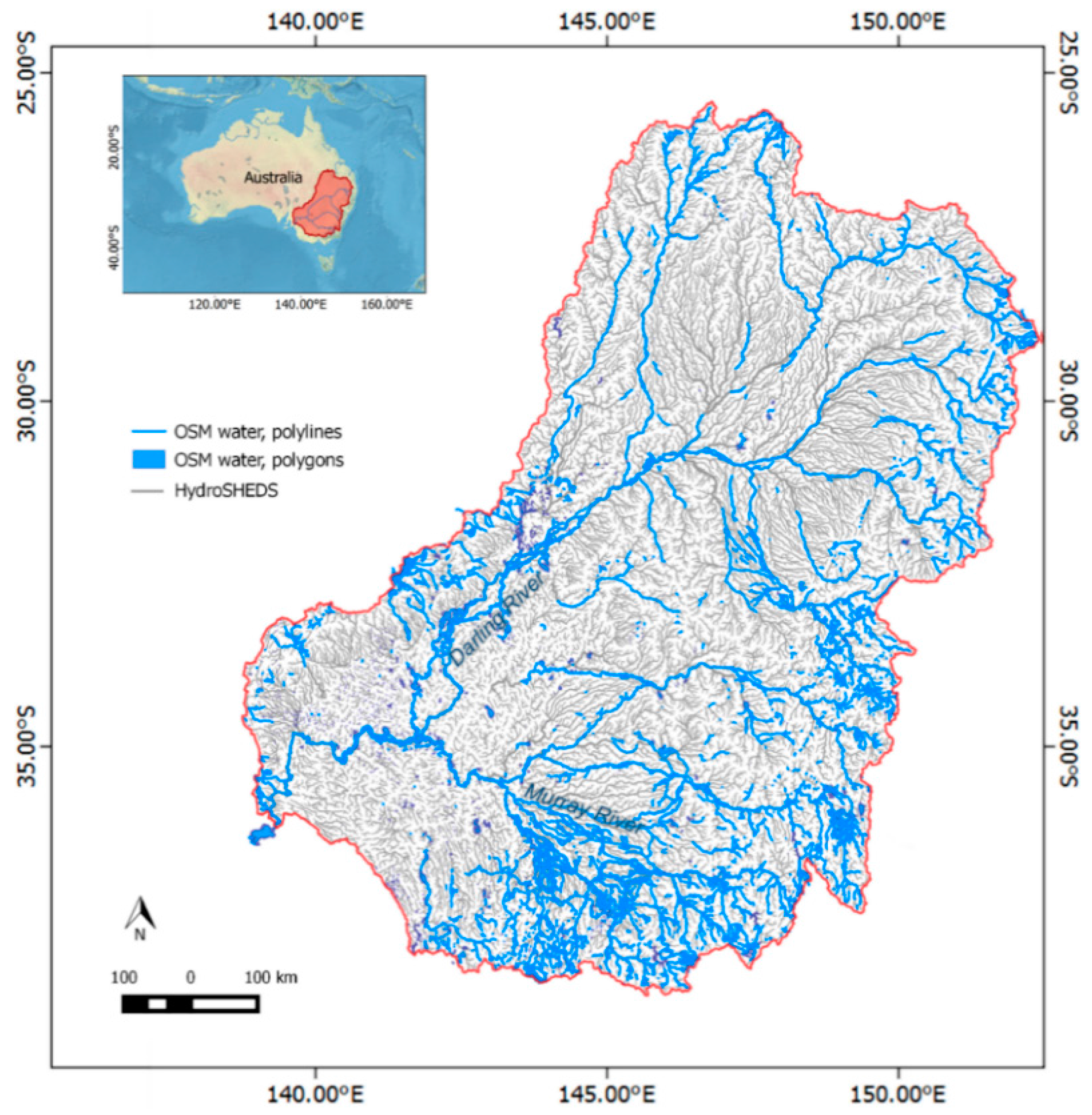
2.1. Study Site: Murray-Darling River Basin
2.2. Input Datasets Used to Extract the Water Mask
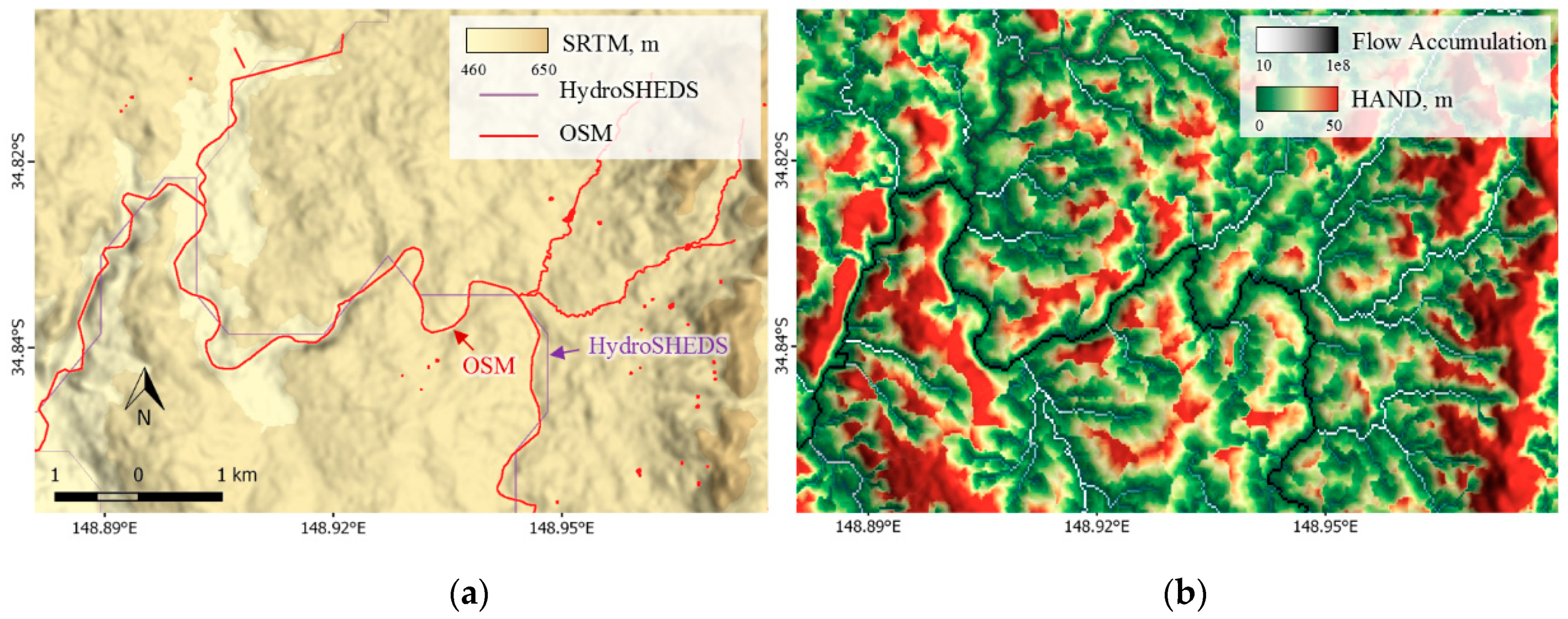
2.3. Derivation of Hydrological Variables: Drainage Network and HAND
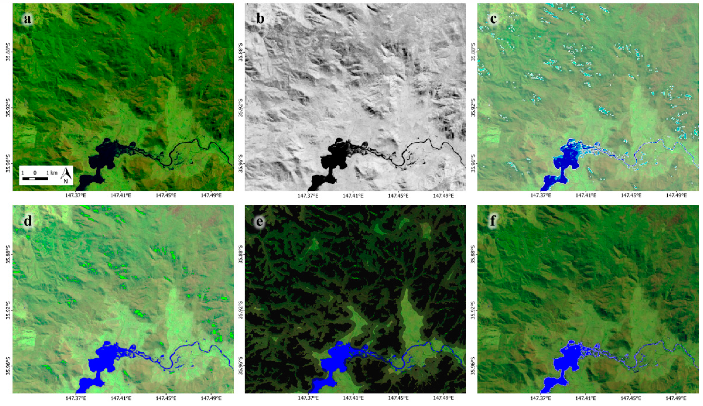
2.4. Method of Water Detection Using Landsat 8
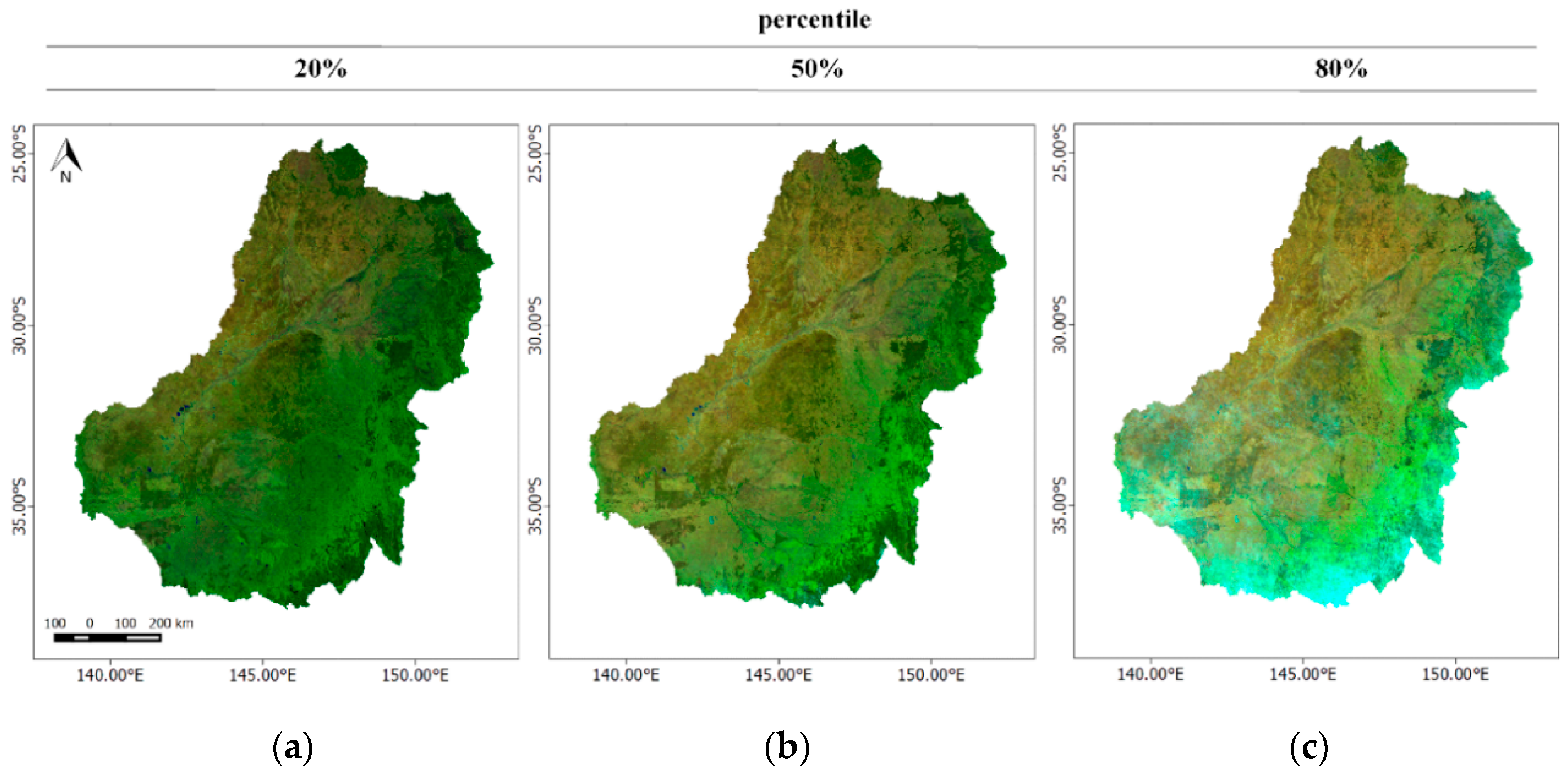
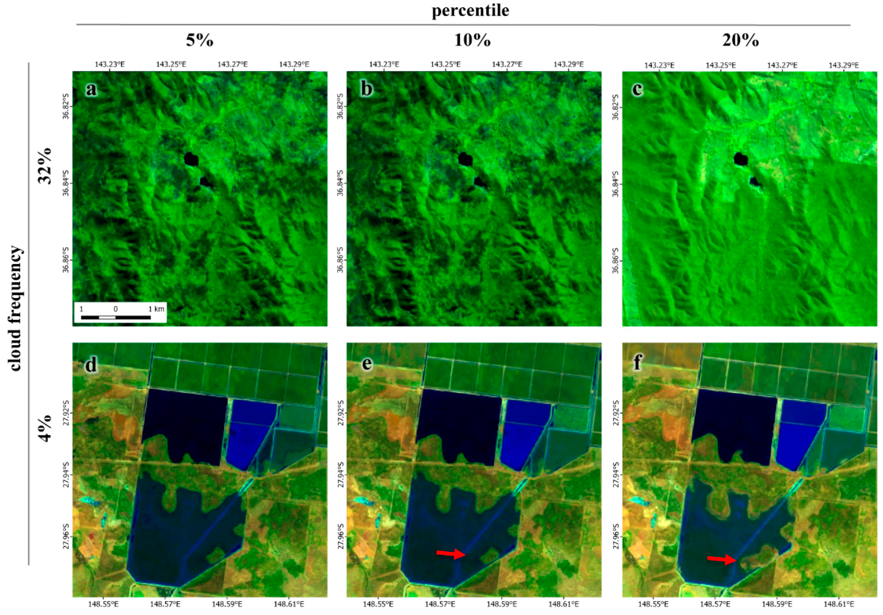
2.4.1. Cloud-Free Landsat 8 Percentile Images
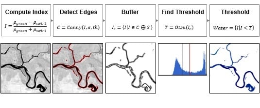
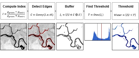
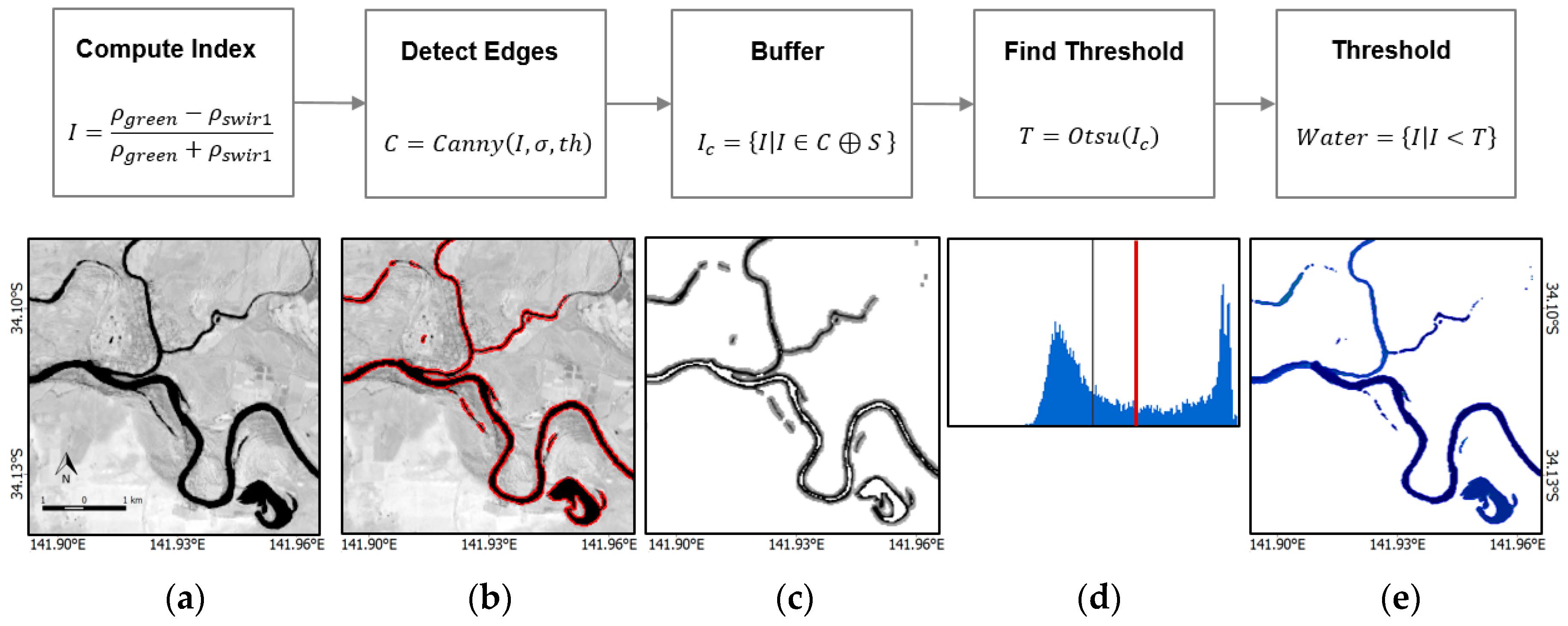
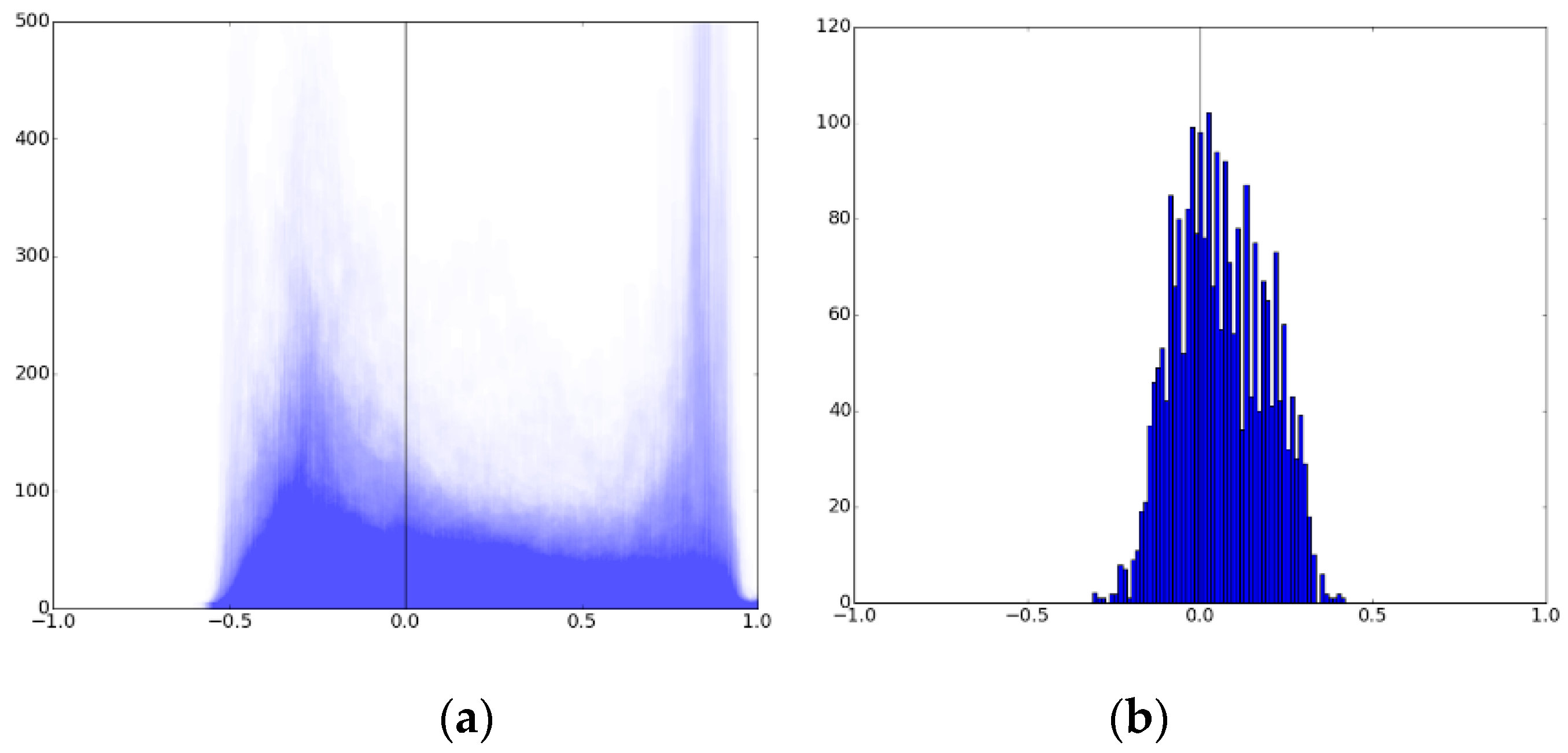
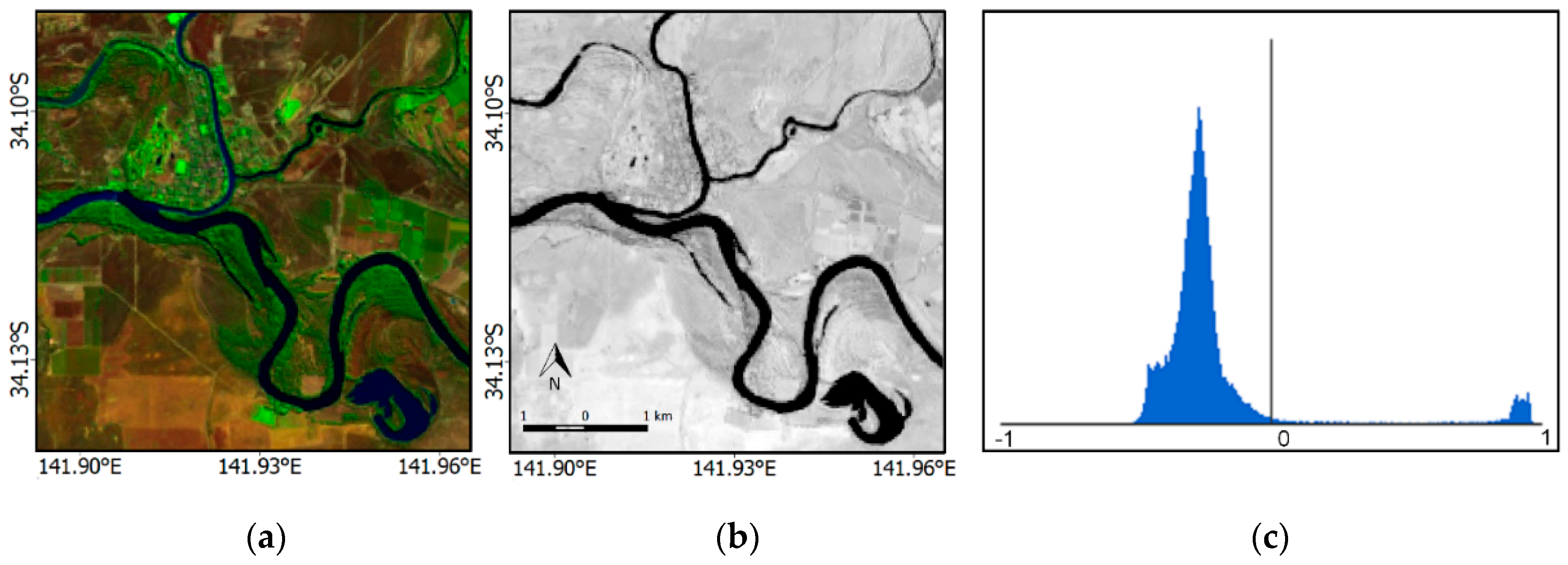
2.4.2. Adaptive Threshold Detection Using MNDWI, Canny Edge Filter, and Otsu Thresholding
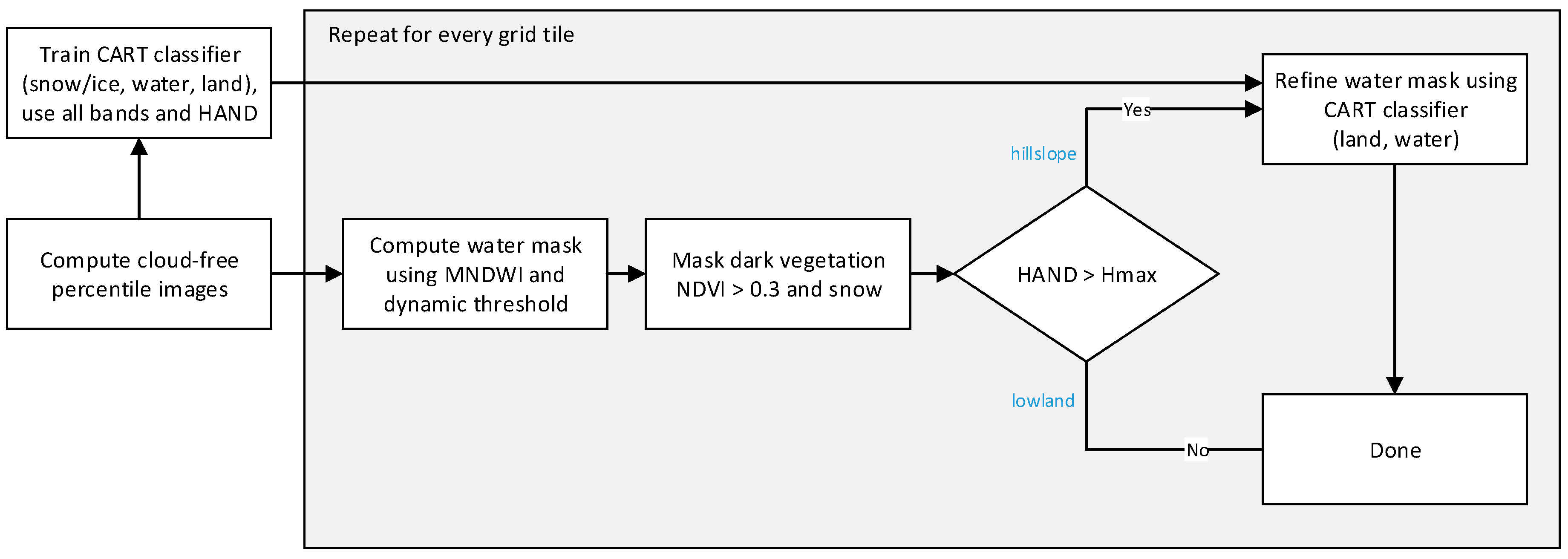
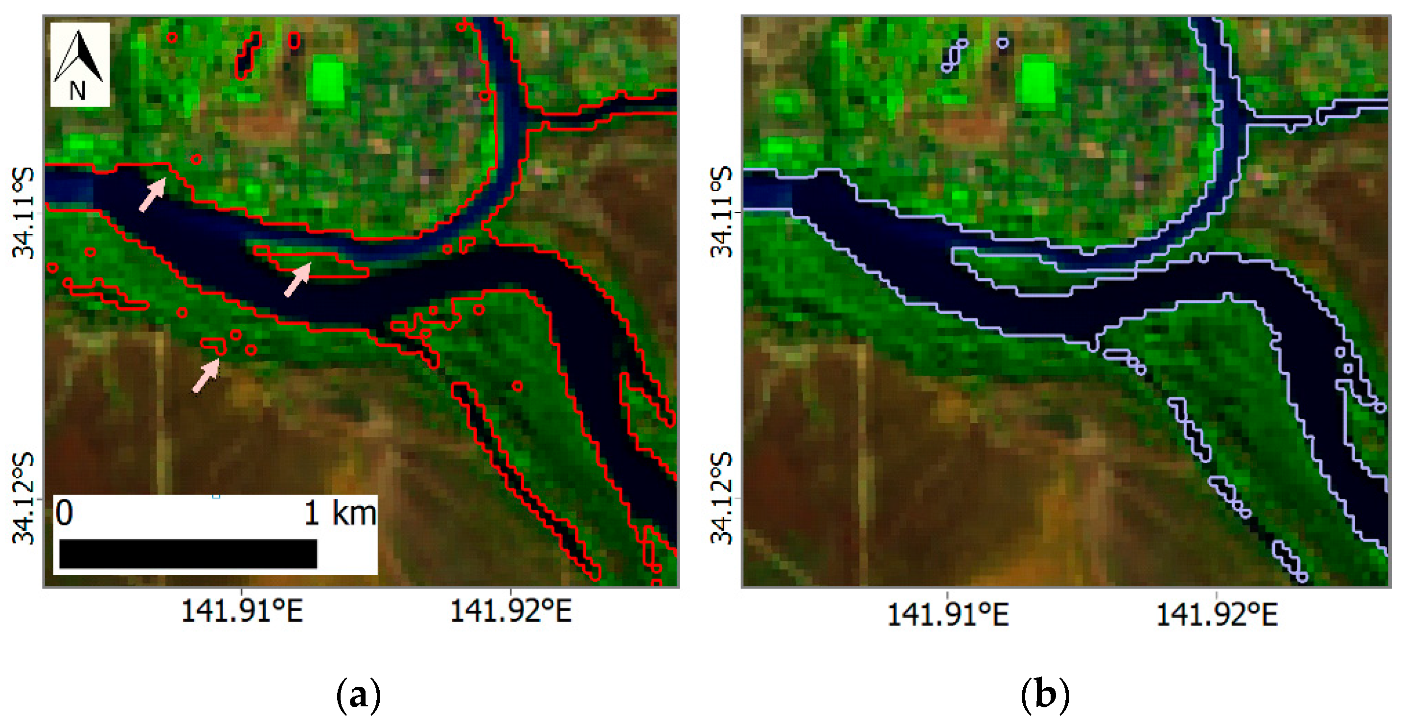
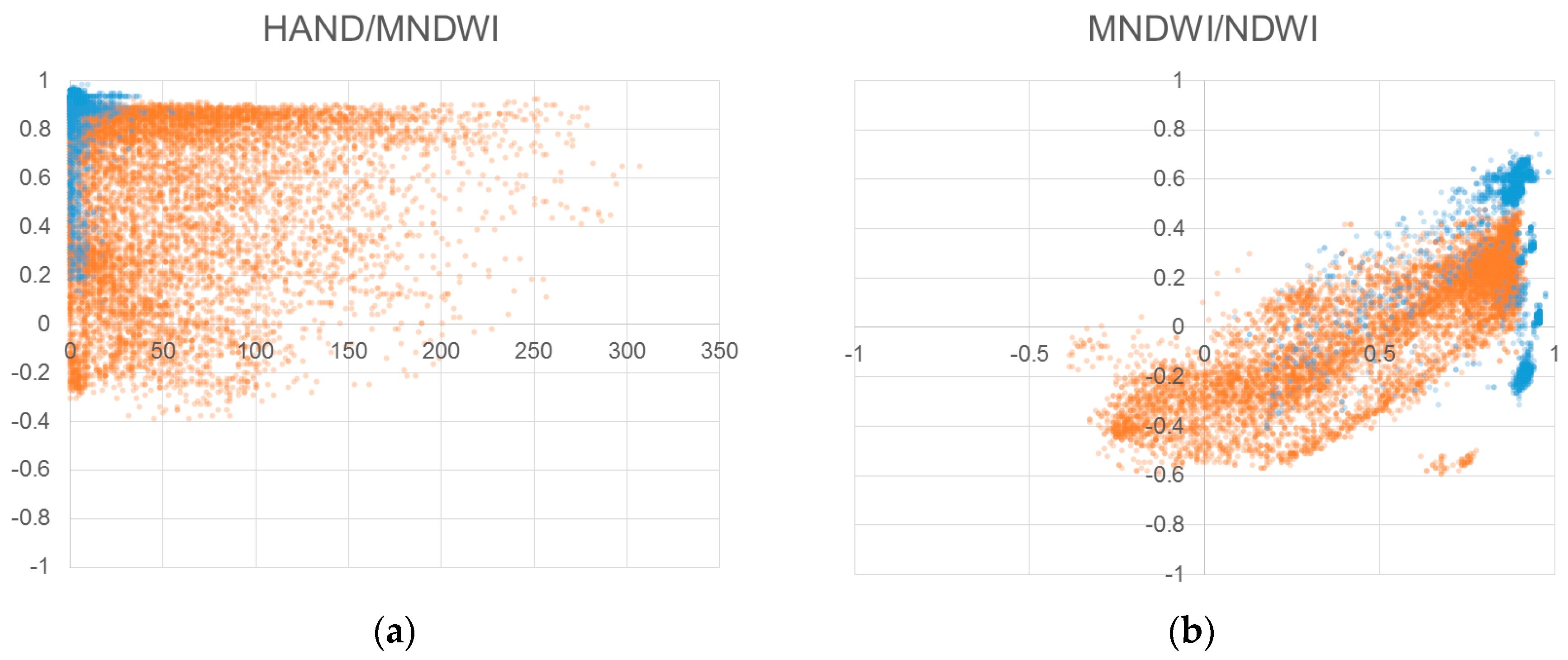
2.4.3. Refining Water Detection Using Supervised Classification Based on CART and HAND
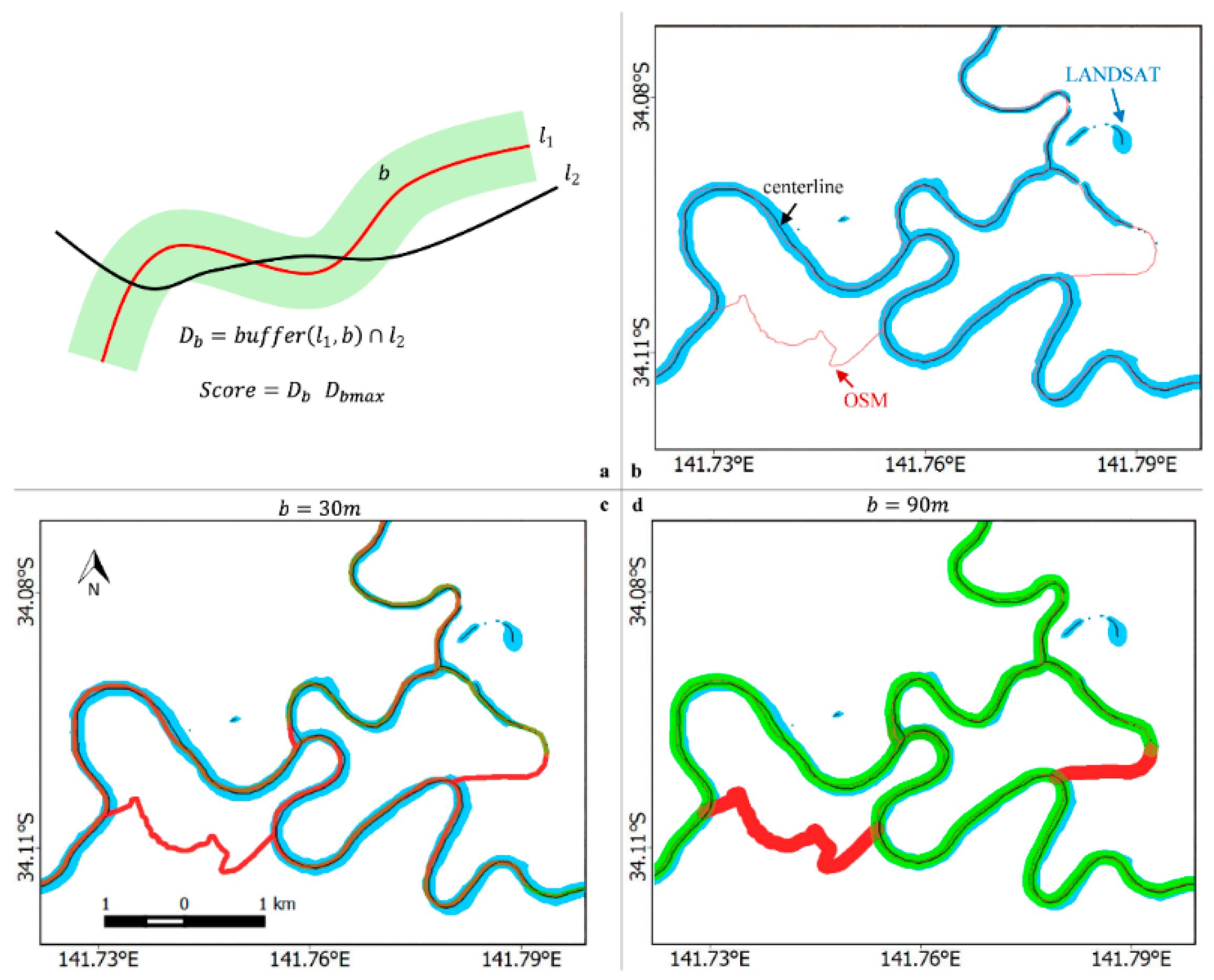
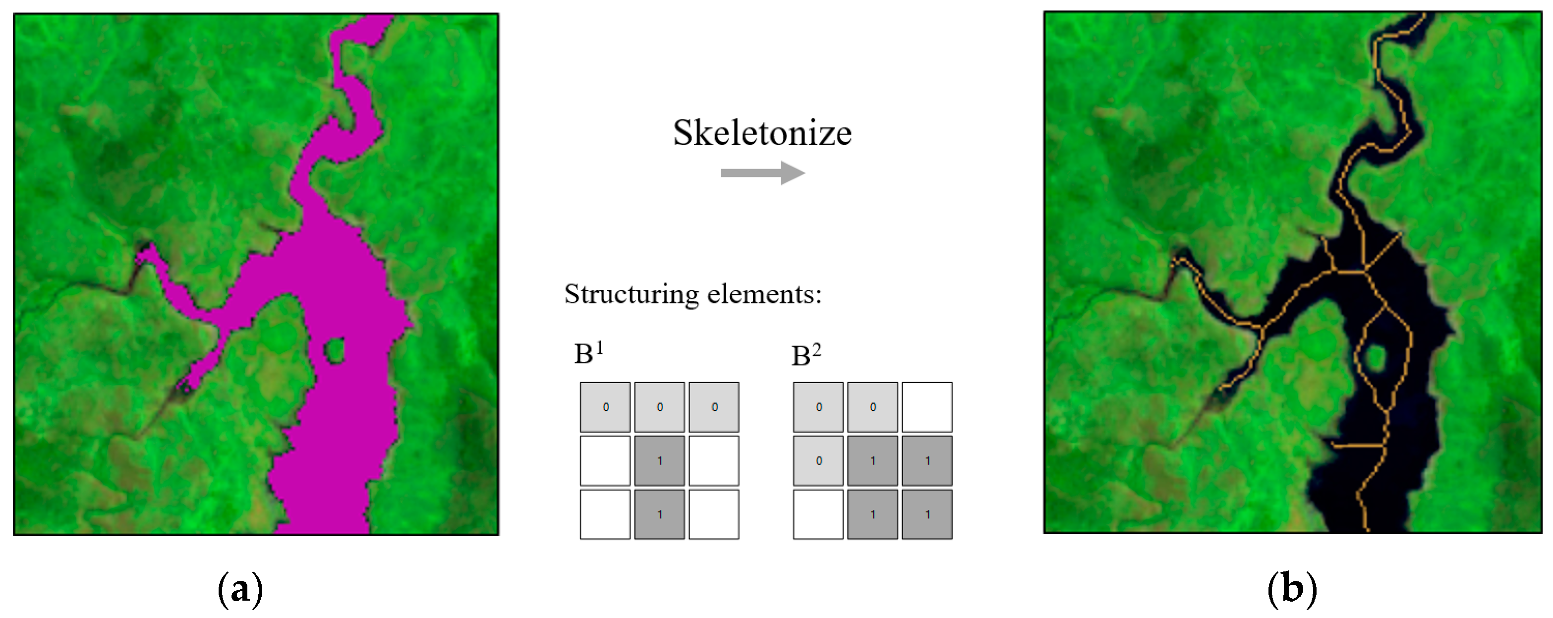
2.5. River Centerline Estimation from Landsat 8 Water Mask
3. Results
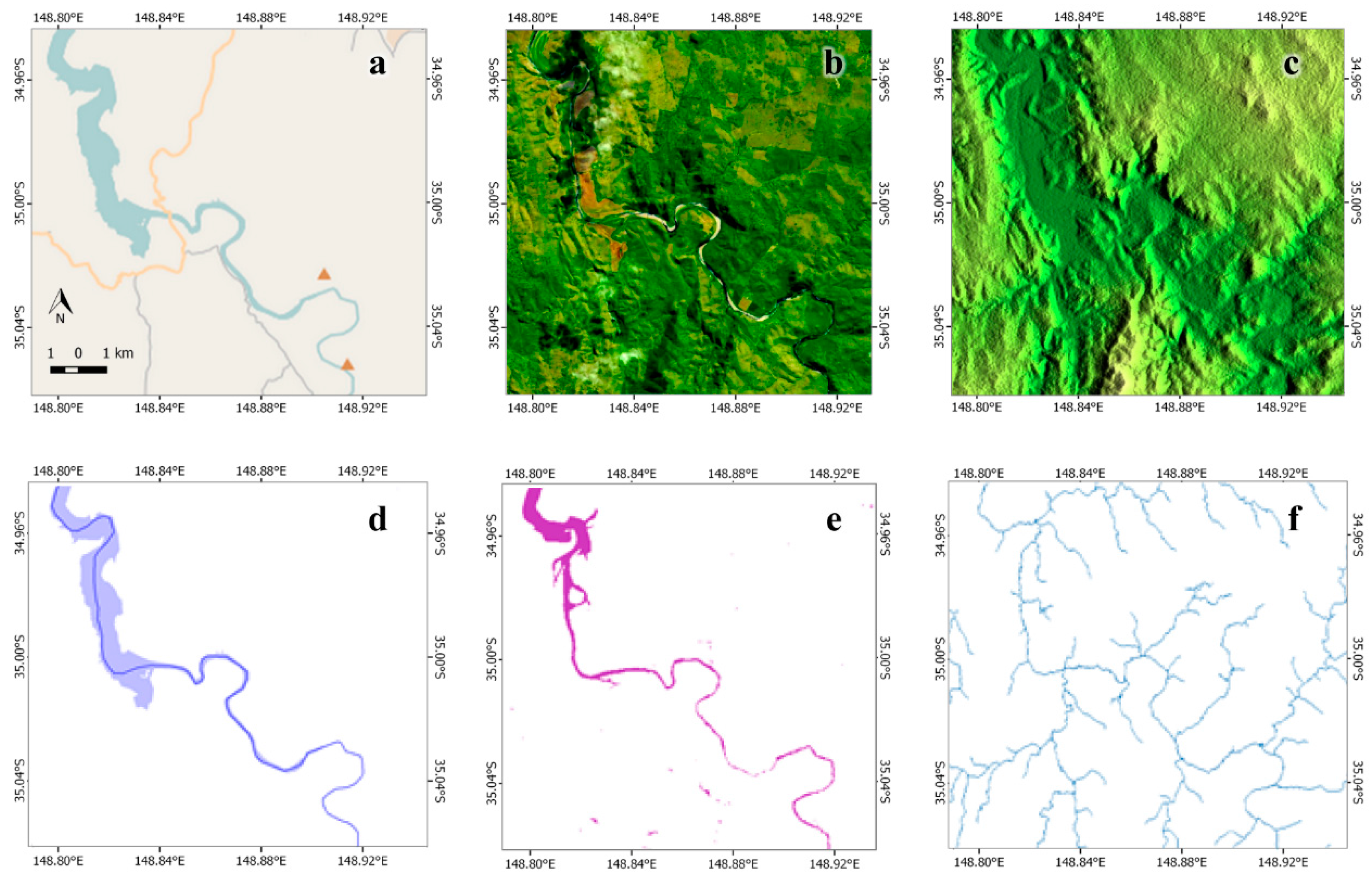
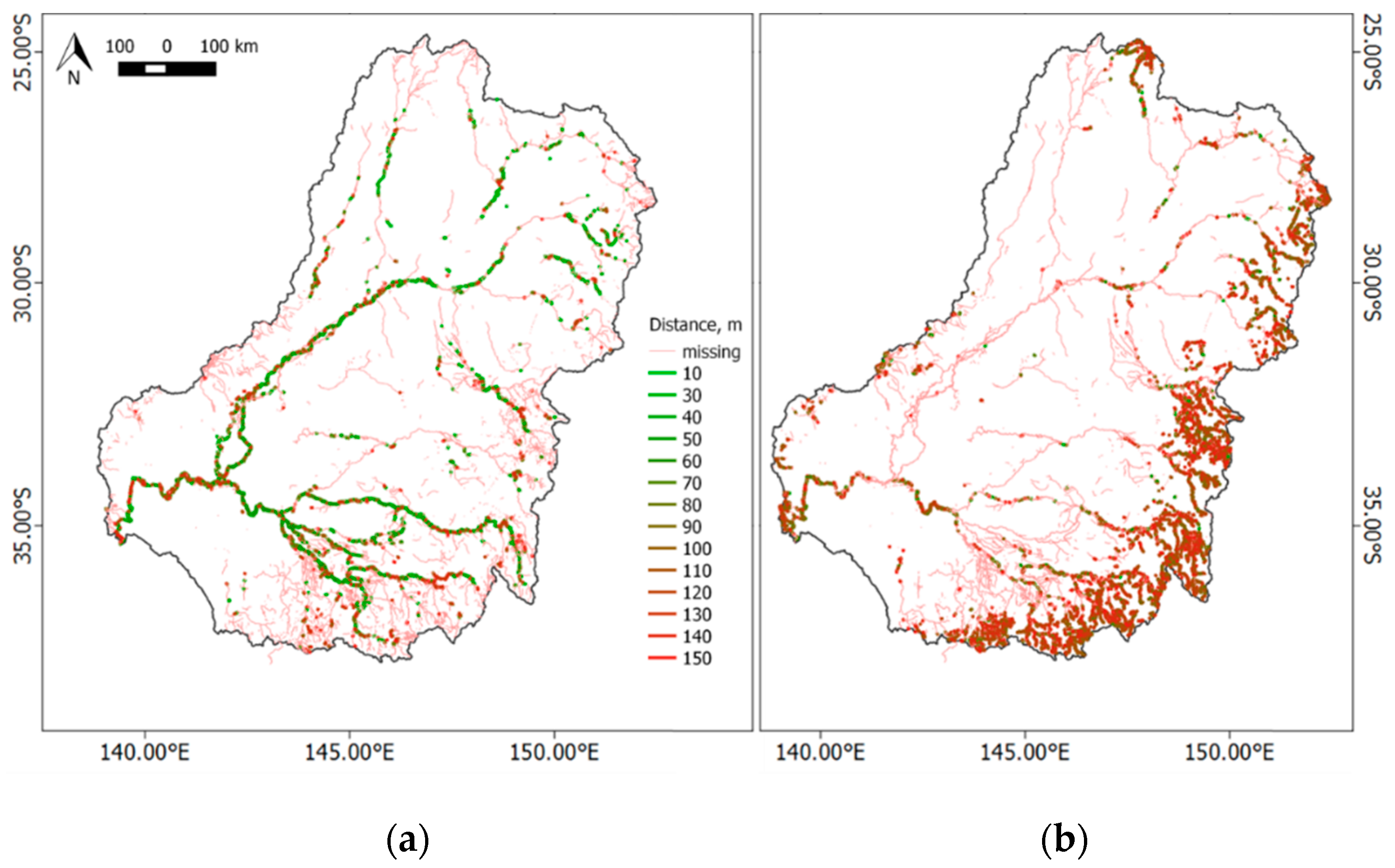
3.1. Estimation of Positional Differences between Rivers
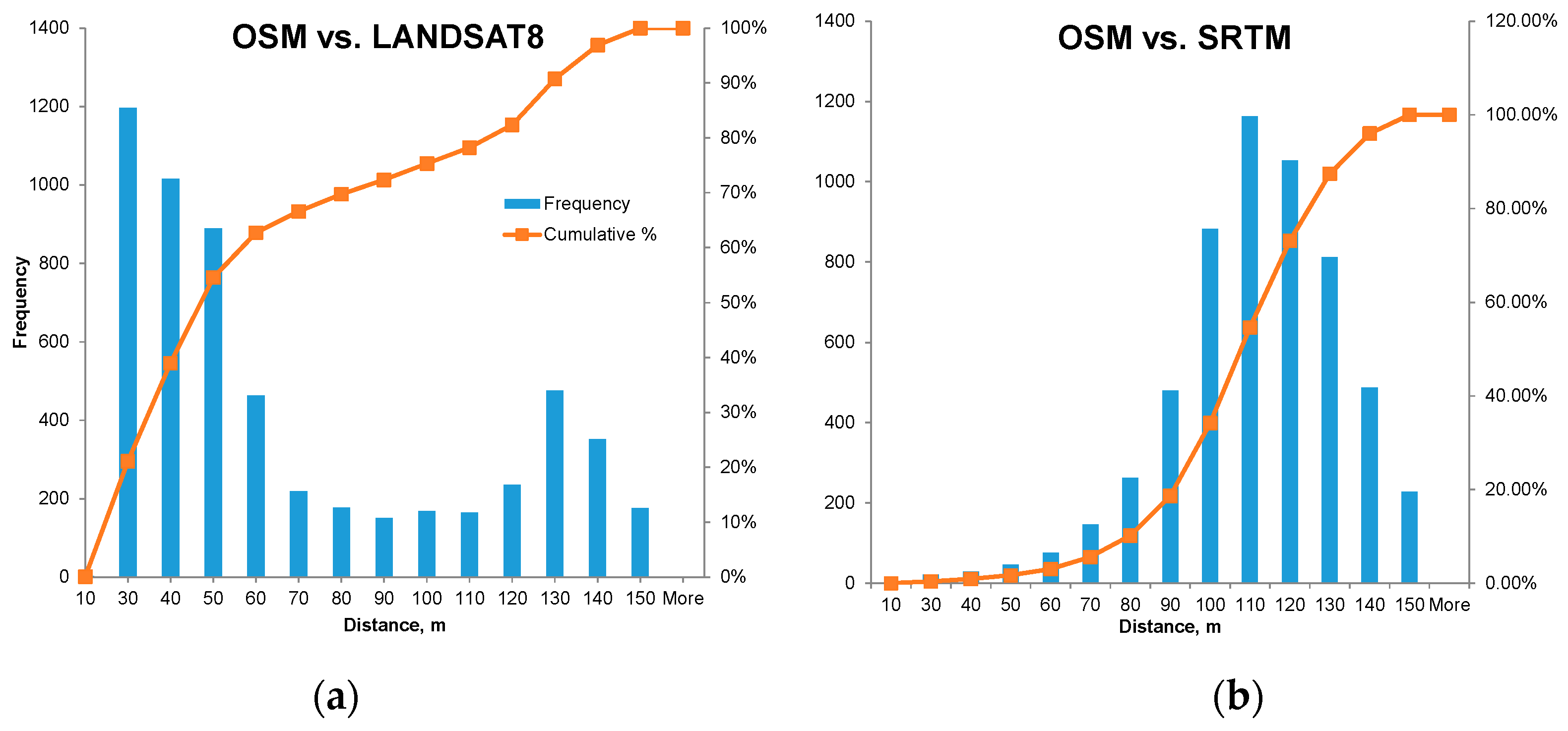
3.2. Positional Differences between OpenStreetMap, Landsat, and SRTM
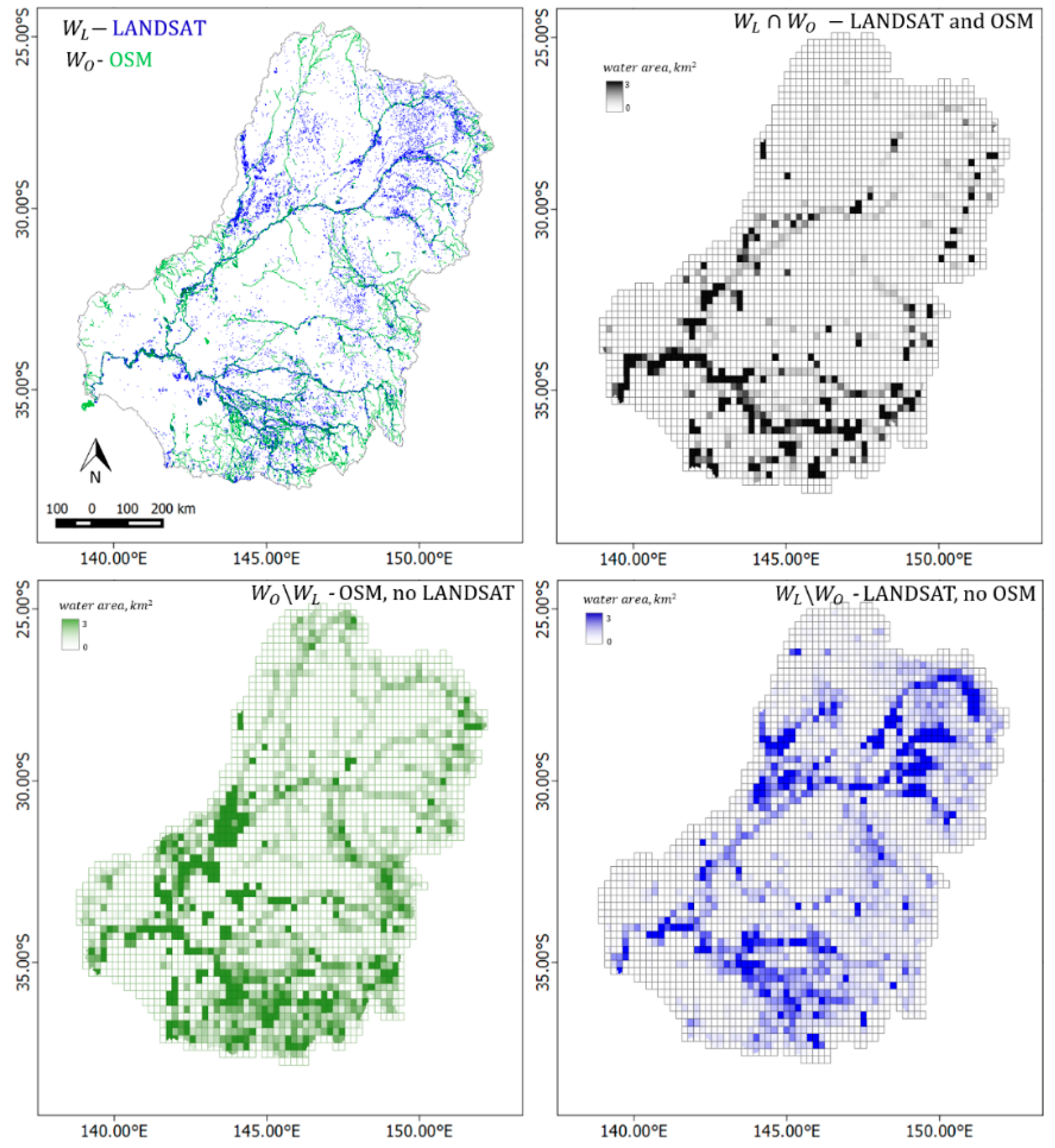
3.3. Goodness of Fit between OpenStreetMap and Landsat Water Masks
4. Discussion
5. Conclusions
Supplementary Materials
Acknowledgments
Author Contributions
Conflicts of Interest
Appendix
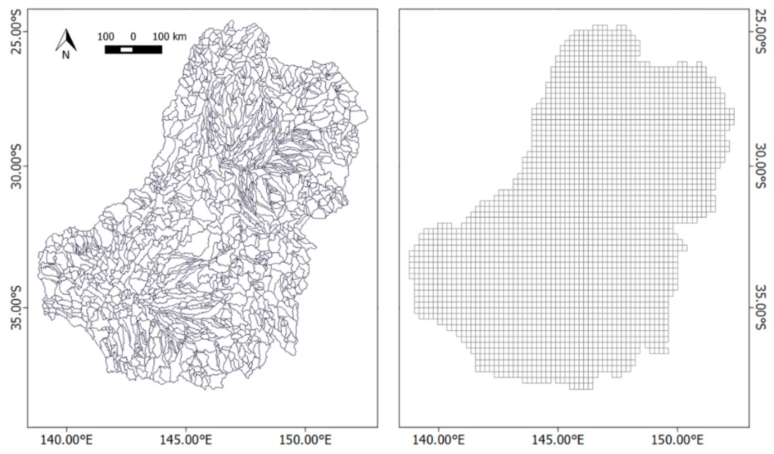
A1. Grids Used During Analysis

A2. Results as Raster and Vector Datasets

| Name | Type | Link |
|---|---|---|
| OpenStreetMap water features for Australia | Fusion Table | [55] |
| HydroBASIN catchments for Australia | Fusion Table | [55] |
| Landsat water mask (raster) | EE Asset | users/gena/AU_Murray_Darling/MNDWI_15_water_WGS |
| Height above the nearest drainage (raster) | EE Asset | users/gena/AU_Murray_Darling/SRTM_30_Murray_Darling_hand |
| Local flow accumulation (raster) | EE Asset | users/gena/AU_Murray_Darling/SRTM_30_Murray_Darling_flow_accumulation |
| Distance to the nearest drainage (raster) | EE Assets | users/gena/AU_Murray_Darling/SRTM_30_Murray_Darling_dist |
| Google Earth Engine script | JavaScript | [56] |
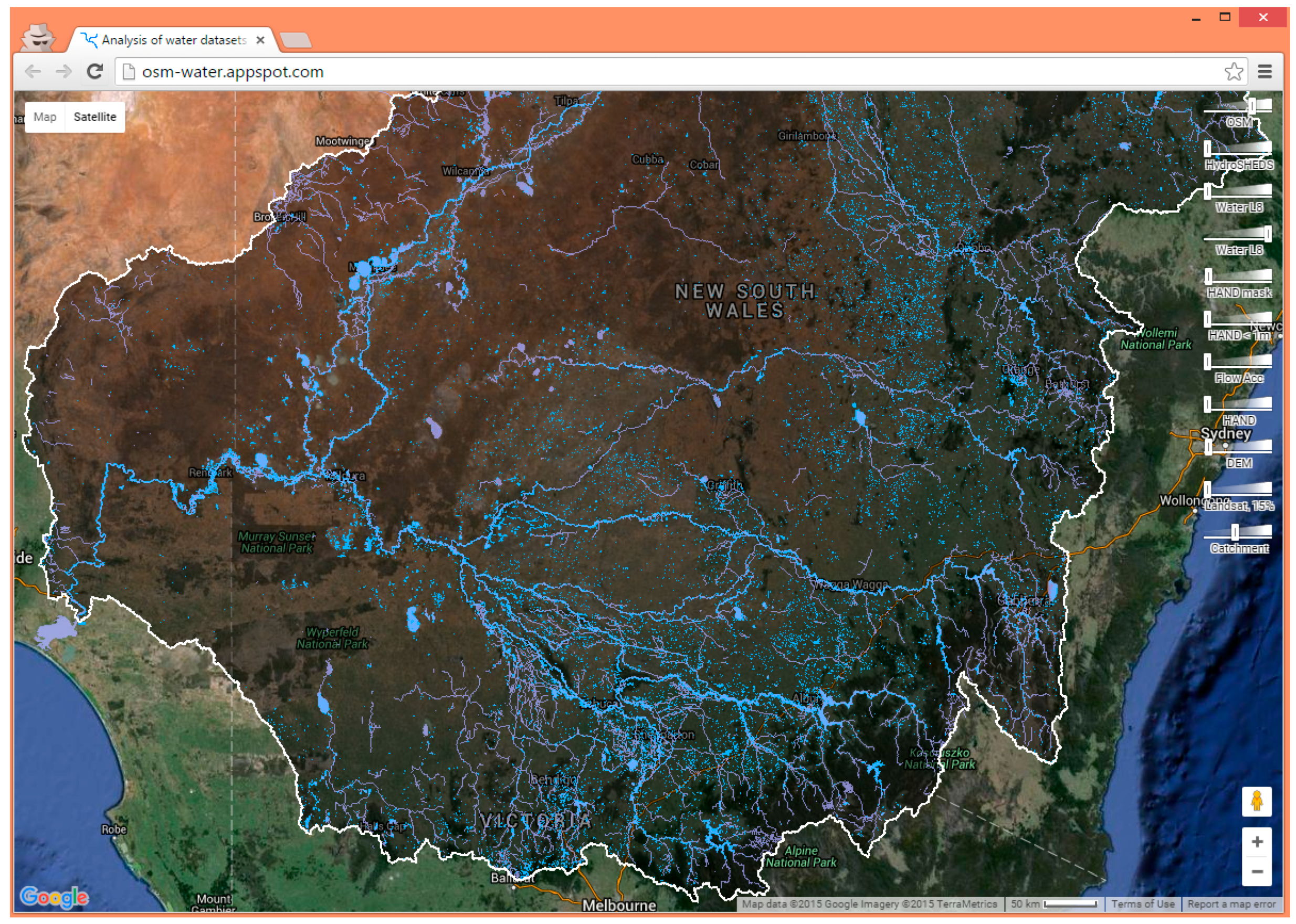
A3. Website
References
- Maidment, D. Arc Hydro: GIS for Water Resources; ESRI Press: Redlands, CA, USA, 2002. [Google Scholar]
- Van Beek, L.; Bierkens, M. The Global Hydrological Model PCR-GLOBWB: Conceptualization, Parameterization and Verification. Available online: http://vanbeek.geo.uu.nl/suppinfo/vanbeekbierkens2009.pdf (accessed on 10 April 2016).
- Wood, E.F.; Roundy, J.K.; Troy, T.J.; van Beek, L.P.H.; Bierkens, M.F.P.; Blyth, E.; de Roo, A.; Döll, P.; Ek, M.; Famiglietti, J.; et al. Hyperresolution global land surface modeling: Meeting a grand challenge for monitoring Earth’s terrestrial water. Water Resour. Res. 2011, 47. [Google Scholar] [CrossRef]
- Bierkens, M.F.P. Global hydrology 2015: State, trends, and directions. Water Resour. Res. 2015, 51, 4923–4947. [Google Scholar] [CrossRef]
- Gao, B.C. NDWI—A normalized difference water index for remote sensing of vegetation liquid water from space. Remote Sens. Environ. 1996, 58, 257–266. [Google Scholar] [CrossRef]
- McFeeters, S.K. The use of the Normalized Difference Water Index (NDWI) in the delineation of open water features. Int. J. Remote Sens. 1996, 17, 1425–1432. [Google Scholar] [CrossRef]
- Xu, H. Modification of normalised difference water index (NDWI) to enhance open water features in remotely sensed imagery. Int. J. Remote Sens. 2006, 27, 3025–3033. [Google Scholar] [CrossRef]
- Zhu, Z.; Woodcock, C.E. Object-based cloud and cloud shadow detection in Landsat imagery. Remote Sens. Environ. 2012, 118, 83–94. [Google Scholar] [CrossRef]
- Zhu, Z.; Woodcock, C.E. Automated cloud, cloud shadow, and snow detection in multitemporal Landsat data: An algorithm designed specifically for monitoring land cover change. Remote Sens. Environ. 2014, 152, 217–234. [Google Scholar] [CrossRef]
- Landsat Higher Level Science Data Products. Available online: http://landsat.usgs.gov/CDR_ECV.php (accessed on 1 January 2016).
- Tan, B.; Masek, J.G.; Wolfe, R.; Gao, F.; Huang, C.; Vermote, E.F.; Sexton, J.O.; Ederer, G. Improved forest change detection with terrain illumination corrected Landsat images. Remote Sens. Environ. 2013, 136, 469–483. [Google Scholar] [CrossRef]
- Potapov, P.V.; Turubanova, S.A.; Hansen, M.C.; Adusei, B.; Broich, M.; Altstatt, A.; Mane, L.; Justice, C.O. Quantifying forest cover loss in Democratic Republic of the Congo, 2000–2010, with Landsat ETM+ data. Remote Sens. Environ. 2012, 122, 106–116. [Google Scholar] [CrossRef]
- Hansen, M.C.; Potapov, P.V.; Moore, R.; Hancher, M.; Turubanova, S.A.; Tyukavina, A.; Thau, D.; Stehman, S.V.; Goetz, S.J.; Loveland, T.R.; et al. High-resolution global maps of 21st-century forest cover change. Science 2013, 342, 850–853. [Google Scholar] [CrossRef] [PubMed]
- Ji, L.; Zhang, L.; Wylie, B. Analysis of dynamic thresholds for the normalized difference water index. Photogramm. Eng. Remote Sens. 2009, 75, 1307–1317. [Google Scholar] [CrossRef]
- Li, W.; Du, Z.; Ling, F.; Zhou, D.; Wang, H.; Gui, Y.; Sun, B.; Zhang, X. A comparison of land surface water mapping using the normalized difference water index from TM, ETM+ and ALI. Remote Sens. 2013, 5, 5530–5549. [Google Scholar] [CrossRef]
- Yang, K.; Li, M.; Liu, Y.; Cheng, L.; Duan, Y.; Zhou, M. River delineation from remotely sensed imagery using a multi-scale classification approach. IEEE J. Sel. Top. Appl. Earth Obs. Remote Sens. 2014, 7, 4726–4737. [Google Scholar] [CrossRef]
- Liu, D.; Yu, J. Otsu method and K-means. In Proceedings of the HIS ′09. Ninth International Conference onHybrid Intelligent Systems, Shenyang, China, 12–14 August 2009.
- Lehner, B.; Verdin, K.; Jarvis, A. New global hydrography derived from spaceborne elevation data. EOS 2008, 89, 93–94. [Google Scholar] [CrossRef]
- Tarboton, D.G. A new method for the determination of flow directions and upslope areas in grid digital elevation models. Water Resour. Res. 1997, 33, 309. [Google Scholar] [CrossRef]
- Rennó, C.D.; Nobre, A.D.; Cuartas, L.A.; Soares, J.V.; Hodnett, M.G.; Tomasella, J.; Waterloo, M.J. HAND, a new terrain descriptor using SRTM-DEM: Mapping terra-firme rainforest environments in Amazonia. Remote Sens. Environ. 2008, 112, 3469–3481. [Google Scholar] [CrossRef]
- Nobre, A.D.; Cuartas, L.A.; Momo, M.R.; Severo, D.L.; Pinheiro, A.; Nobre, C.A. HAND contour: A new proxy predictor of inundation extent. Hydrol. Process. 2016, 30, 320–333. [Google Scholar] [CrossRef]
- Manfreda, S.; Nardi, F.; Samela, C.; Grimaldi, S.; Taramasso, A.C.; Roth, G.; Sole, A. Investigation on the use of geomorphic approaches for the delineation of flood prone areas. J. Hydrol. 2014, 517, 863–876. [Google Scholar] [CrossRef]
- Eilander, D.; Annor, F.O.; Iannini, L.; van de Giesen, N. Remotely sensed monitoring of small reservoir dynamics: A Bayesian approach. Remote Sens. 2014, 6, 1191–1210. [Google Scholar] [CrossRef]
- Haklay, M. How good is volunteered geographical information? A comparative study of OpenStreetMap and ordnance survey datasets. Environ. Plan. B Plan. Des. 2010, 37, 682–703. [Google Scholar] [CrossRef]
- OpenStreetMap Taginfo. Available online: http://taginfo.openstreetmap.org/tags (accessed on 24 November 2015).
- Schellekens, J.; Brolsma, R.J.; Dahm, R.J.; Donchyts, G.V.; Winsemius, H.C. Rapid setup of hydrological and hydraulic models using OpenStreetMap and the SRTM derived digital elevation model. Environ. Model. Softw. 2014, 61, 98–105. [Google Scholar] [CrossRef]
- Mooney, P.; Corcoran, P.; Winstanley, A.C. Towards quality metrics for OpenStreetMap. In Proceedings of the 18th SIGSPATIAL International Conference on Advances in Geographic Information, New York, NY, USA, 5–7 September 2010.
- Girres, J.F.; Touya, G. Quality Assessment of the French OpenStreetMap Dataset. Trans. GIS 2010, 14, 435–459. [Google Scholar] [CrossRef]
- Goodchild, M.F.; Hunter, G.J. A simple positional accuracy measure for linear features. Int. J. Geogr. Inf. Sci. 1997, 11, 299–306. [Google Scholar] [CrossRef]
- Barron, C.; Neis, P.; Zipf, A. A comprehensive framework for intrinsic OpenStreetMap quality analysis. Trans. GIS 2014, 18, 877–895. [Google Scholar] [CrossRef]
- International Organization for Standardization: ISO 19113:2002: Geographic Information—Quality Principles. Available online: http://www.iso.org/iso/catalogue_detail.htm?csnumber=26018 (accessed on 10 April 2016).
- Crossman, S.; Li, O. Surface Hydrology Lines (Regional), 2nd ed.Australia. Available online: http://www.ga.gov.au/metadata-gateway/metadata/record/83130 (accessed on 5 April 2016).
- Mueller, N.; Lewis, A.; Roberts, D.; Ring, S.; Melrose, R.; Sixsmith, J.; Lymburner, L.; McIntyre, A.; Tan, P.; Curnow, S.; et al. Water observations from space: Mapping surface water from 25 years of Landsat imagery across Australia. Remote Sens. Environ. 2015, 174, 341–352. [Google Scholar] [CrossRef]
- Digital Elevation Model (DEM) of Australia Derived from LiDAR 5 Metre Grid. Geoscience Australia, Canberra. Available online: http://dx.doi.org/10.4225/25/5652419862E23 (accessed on 5 April 2016).
- Roy, D.P.; Wulder, M.A.; Loveland, T.R.; Woodcock, C.E.; Allen, R.G.; Anderson, M.C.; Helder, D.; Irons, J.R.; Johnson, D.M.; Kennedy, R.; et al. Landsat-8: Science and product vision for terrestrial global change research. Remote Sens. Environ. 2014, 145, 154–172. [Google Scholar] [CrossRef]
- NASA Shuttle Radar Topography Mission. Available online: http://www2.jpl.nasa.gov/srtm/ (accessed on 24 November 2015).
- Murray-Darling Basin Authority. Available online: http://www.mdba.gov.au/about-basin (accessed on 1 January 2016).
- Natural Earth Map Dataset. Available online: http://www.naturalearthdata.com/ (accessed on 5 April 2016).
- OpenStreetMap Planet File. Available online: http://planet.osm.org/ (accessed on 24 November 2015).
- Lehner, B.; Grill, G. Global river hydrography and network routing: Baseline data and new approaches to study the world’s large river systems. Hydrol. Process. 2013, 27, 2171–2186. [Google Scholar] [CrossRef]
- Warmerdam, F. The Geospatial Data Abstraction Library. Available online: http://link.springer.com/chapter/10.1007/978-3-540-74831-1_5 (accessed on 15 January 2016).
- O’Callaghan, J.; Mark, D. The extraction of drainage networks from digital elevation data. Comput. Vis. Graph. Image Process. 1984, 28, 323–344. [Google Scholar] [CrossRef]
- Karssenberg, D.; Schmitz, O. A software framework for construction of process-based stochastic spatio-temporal models and data assimilation. Environ. Model. Softw. 2010, 25, 489–502. [Google Scholar] [CrossRef]
- PCRaster Web Page. Available online: http://pcraster.geo.uu.nl/ (accessed on 1 May 2016).
- Tucker, C.J. Red and photographic infrared linear combinations for monitoring vegetation. Remote Sens. Environ. 1979, 8, 127–150. [Google Scholar] [CrossRef]
- Breiman, L.; Friedman, J.; Stone, C.; Olshen, R. Classification and Regression Trees, 1st ed.; Chapman and Hall/CRC: Boca Raton, FL, USA, 1984. [Google Scholar]
- Rodriguez, E.; Morris, C.; Belz, J. An assessment of the SRTM topographic products. Photogramm. Eng. Remote Sens. 2006, 72, 249–260. [Google Scholar]
- Gorelick, N. Google Earth Engine. Available online: http://adsabs.harvard.edu/abs/2012AGUFM.U31A..04G (accessed on 28 April 2016).
- Google Fusion Table Web Page. Available online: http://tables.googlelabs.com (accessed on 1 May 2016).
- Serra, J. Image Analysis and Mathematical Morphology; Academic Press, Inc.: Orlando, FL, USA, 1982; Volume 1. [Google Scholar]
- Fiona GitHub Web Page. Available online: https://github.com/Toblerity/Fiona (accessed on 28 March 2016).
- Shapely GitHub Web Page. Available online: https://github.com/Toblerity/Shapely (accessed on 1 January 2016).
- Ee-Runner GitHub Web Page. Available online: https://github.com/gena/ee-runner (accessed on 1 January 2016).
- Supplementary GitHub Repository Web Page. Available online: http://github.com/gena/paper-osm-2015 (accessed on 1 May 2016).
- Supplementary Google Fusion Tables Web Page. Available online: http://bit.ly/paper-osm-2016-fusion-tables (accessed on 1 May 2016).
- Supplementary Google Earth Engine Script Web Page. Available online: http://bit.ly/paper-osm-2016-gee-assets (accessed on 1 May 2016).
- Supplementary Project Web Page. Available online: http://osm-water.appspot.com (accessed on 1 May 2016).


| Dataset | Type | Resolution | Notes |
|---|---|---|---|
| Landsat 8 TOA | Multispectral Imagery | 15 m, 30 m, 60 m | 2743 scenes were used, acquired during 2013–2015, top of atmosphere (TOA) reflectance. |
| SRTM | Elevation Imagery | 30 m | Effective resolution is lower due to the presence of high-frequency noise |
| OpenStreetMap | Polyline and Polygon Vector | 1–100 m | Planet file from August 2015, the following tags query was used to indicate water features: natural = water or natural = spring or waterway = or landuse = basin or landuse = reservoir or barrier = ditch or landuse = saltpond |
| HydroBASINS | Polygons | ~450 m | Level 8 basins were used to delineate HAND using 30 m version of SRTM |
| Variable | Area, km2 | Ratio, % | |||
|---|---|---|---|---|---|
| 8981 | 100% | ||||
| 7073 | 79% | ||||
| 4799 | 53% | ||||
| 2891 | 32% | ||||
| 4182 | 47% | ||||
| 1908 | 21% | ||||
© 2016 by the authors; licensee MDPI, Basel, Switzerland. This article is an open access article distributed under the terms and conditions of the Creative Commons Attribution (CC-BY) license (http://creativecommons.org/licenses/by/4.0/).
Share and Cite
Donchyts, G.; Schellekens, J.; Winsemius, H.; Eisemann, E.; Van de Giesen, N. A 30 m Resolution Surface Water Mask Including Estimation of Positional and Thematic Differences Using Landsat 8, SRTM and OpenStreetMap: A Case Study in the Murray-Darling Basin, Australia. Remote Sens. 2016, 8, 386. https://doi.org/10.3390/rs8050386
Donchyts G, Schellekens J, Winsemius H, Eisemann E, Van de Giesen N. A 30 m Resolution Surface Water Mask Including Estimation of Positional and Thematic Differences Using Landsat 8, SRTM and OpenStreetMap: A Case Study in the Murray-Darling Basin, Australia. Remote Sensing. 2016; 8(5):386. https://doi.org/10.3390/rs8050386
Chicago/Turabian StyleDonchyts, Gennadii, Jaap Schellekens, Hessel Winsemius, Elmar Eisemann, and Nick Van de Giesen. 2016. "A 30 m Resolution Surface Water Mask Including Estimation of Positional and Thematic Differences Using Landsat 8, SRTM and OpenStreetMap: A Case Study in the Murray-Darling Basin, Australia" Remote Sensing 8, no. 5: 386. https://doi.org/10.3390/rs8050386
APA StyleDonchyts, G., Schellekens, J., Winsemius, H., Eisemann, E., & Van de Giesen, N. (2016). A 30 m Resolution Surface Water Mask Including Estimation of Positional and Thematic Differences Using Landsat 8, SRTM and OpenStreetMap: A Case Study in the Murray-Darling Basin, Australia. Remote Sensing, 8(5), 386. https://doi.org/10.3390/rs8050386