Spectral-Spatial Hyperspectral Image Classification Using Subspace-Based Support Vector Machines and Adaptive Markov Random Fields

Abstract

This paper introduces a new supervised classification method for hyperspectral images that combines spectral and spatial information. A support vector machine (SVM) classifier, integrated with a subspace projection method to address the problems of mixed pixels and noise, is first used to model the posterior distributions of the classes based on the spectral information. Then, the spatial information of the image pixels is modeled using an adaptive Markov random field (MRF) method. Finally, the maximum posterior probability classification is computed via the simulated annealing (SA) optimization algorithm. The combination of subspace-based SVMs and adaptive MRFs is the main contribution of this paper. The resulting methods, called SVMsub-eMRF and SVMsub-aMRF, were experimentally validated using two typical real hyperspectral data sets. The obtained results indicate that the proposed methods demonstrate superior performance compared with other classical hyperspectral image classification methods.

1. Introduction

In recent years, immense research efforts have been devoted to hyperspectral image classification. Given a set of observations (i.e., pixel vectors in a hyperspectral image), the goal of classification is to assign a unique label to each pixel vector such that it can be identified as belonging to a given class [1]. Classification techniques can be divided into unsupervised and supervised approaches, of which supervised classification methods are more widely used. However, the supervised classification of high-dimensional data sets, especially hyperspectral images, remains a challenging endeavor [2]. The Hughes phenomenon caused by the imbalance between the large number of spectral bands and the limited availability of training samples poses a major problem during this process. Additionally, the presence of noise and that of mixed pixels, affected by the spatial resolution, represent further hurdles hindering accurate hyperspectral image classification. To address these problems, machine learning models have been combined with several methods of feature dimension reduction that are able to produce accurate results, including support vector machines (SVMs) [3,4] and subspace projection methods [5,6].

Subspace projection methods have been shown to be a powerful tool in reducing the dimensionality of input data [7]. The fundamental idea of such a method is to project the original pixel vector to a lower-dimensional subspace that is spanned by a set of basis vectors. The details of subspace projection methods and the framework thereof are presented in Section 3.1. Recently, several approaches using subspace-based techniques have been exploited for hyperspectral image classification. In [8], an SVM nonlinear function called subspace-based SVM (SVMsub) was constructed by using the subspaces associated with each class for classification. In [9], a classifier that couples nearest-subspace classification with distance-weighted Tikhonov regularization was proposed for hyperspectral imagery. In [10], a subspace-based technique in a multinomial logistic regression (MLR) framework, called MLRsub, was developed to characterize mixed pixels in hyperspectral data. A general conclusion drawn from the aforementioned studies is that subspace projection methods are useful for reducing dimensionality by transforming the input data to the desired subspaces without loss of information. Additionally, such methods are suitable for the separation of classes that are spectrally similar because of spectral mixing and other reasons.

Another recent trend in attempts to improve classification accuracy is to combine spectral and spatial information [11,12,13]. On the one hand, Benediktsson et al. presented a series of studies of the integration of morphological features with segmentation techniques for the spectral-spatial classification of hyperspectral data [14,15]. The reported experiments proved that the proposed methods can yield promising results with high accuracy. On the other hand, the Markov random field (MRF) approach has also been proven to be an effective method of addressing spectral and spatial information. The basic principle of the MRF method is to integrate the spatial correlation information into the posterior probability distribution of the spectral features. Thus, this method can produce an accurate feature representation of pixels and their neighborhoods. Further details on the MRF method and its enhancement are presented in Section 2.2. In [16], a new supervised segmentation algorithm for remotely sensed hyperspectral image data was introduced that integrates a subspace-based MLR algorithm with a multilevel logistic Markov–Gibbs MRF prior; this algorithm is called MLRsub-MRF. To further improve the ability to characterize spatial information using the MRF approach, adaptive techniques have been applied to the spatial term to develop adaptive MRF methods. In [17], an edge-constrained MRF method (eMRF) was proposed for accurate land-cover classification over urban areas using hyperspectral imagery. In [18], an adaptive MRF approach that uses a relative homogeneity index (RHI) to characterize the spatial contribution was proposed for the classification of hyperspectral imagery; this method is called aMRF. Further details on these two methods are presented in Section 3.2 and Section 3.3.

As mentioned above, subspace projection methods can be used to efficiently improve the classification accuracy of algorithms such as those based on SVMs and MLR, which predominantly use information from the spectral domain [8,10]. Moreover, through the combination of MRF models and MLRsub, it has been proven that spatial correlation information is also useful for algorithms based on subspace projection [16]. A previous experimental comparison has shown that SVMsub outperforms MLRsub [8]. Therefore, we can integrate MRF models with SVMsub to achieve a higher classification accuracy than that offered by the MLRsub-MRF algorithm proposed in [16]. Furthermore, we improve our MRF modeling by using the adaptive strategy introduced in our previous works [17,18] to propose two novel algorithms called SVMsub-eMRF (SVMsub combined with the eMRF method proposed in [17]) and SVMsub-aMRF (SVMsub combined with the RHI-based aMRF method proposed in [18]). Compared with SVMsub and MLRsub-MRF, the main advantages and contributions of this work lie in the design and improvement of the classification algorithms through optimization in both the spectral and spatial domains. In the spectral domain, SVMsub can obtain results with higher accuracy than MLRsub, and eMRF and aMRF also demonstrate better performance than conventional MRF models.

Our method is implemented in two steps: (1) a learning step, in which the posterior probability distribution and pre-classification results are obtained using an SVM classifier integrated with a subspace projection method; and (2) a post-processing step, in which the class labels computed during the pre-classification process are revised via an adaptive MRF approach. The final result is optimized using the simulated annealing (SA) optimization algorithm [19]. The proposed method not only can cope with the Hughes phenomenon and the effect of mixed pixels but also is able to discriminatively address the relationships exhibited by pixels in homogeneous regions or on boundaries. We performed experiments to compare the performances of two adaptive MRF algorithms, the edge-constraint-based eMRF algorithm [17] and the RHI-based aMRF algorithm [18], and both of them achieved superior accuracies compared with other spectral-spatial hyperspectral image classifiers. In addition to these advantages, our approach also provides a fast computation speed by virtue of the subspace-based SVM analysis.

The remainder of this paper is organized as follows. Section 2 introduces the classical SVM model and MRF algorithm, along with some analysis of the problems encountered in their application to hyperspectral data sets. Section 3 presents the proposed classification method combining the subspace-based SVM approach and the adaptive MRF approach. Section 4 evaluates the performances of our methods compared with those of other hyperspectral image classifiers, using data sets collected by the Airborne Visible/Infrared Imaging Spectrometer (AVIRIS) over the Indian Pines region in Indiana and by the Reflective Optics Spectrographic Imaging System (ROSIS) over the University of Pavia in Italy. Section 5 presents some concluding remarks.

2. Related Work

In this section, we introduce two basic components of our framework. The classical SVM model is introduced in Section 2.1, along with an analysis of its application to hyperspectral images. Section 2.2 presents the concept of MRFs and an introduction to the improvement achieved using this approach.

2.1. SVM Model

Consider a hyperspectral image data set $x\equiv \{x_1,x_2,\mathbf{\dots },x_n\}$, where $n$ is the total number of pixels, $x_i={[x_{i1},x_{i2},\dots ,x_{id}]}^T$ denotes the spectral vector associated with an image pixel $i$, and $d$ is the number of spectral bands. Let $y\equiv (y_1,y_2,\dots y_n)$ and $\mathrm{{\rm K}}\equiv \{1,\dots ,K\}$, where $K$ is the total number of classes. If $y_i{}^{(k)}=1$ and $y_i{}^{(c)}=-1$ for $c\in \{\mathrm{{\rm K}}|c\ne k\}$, then pixel $i$ belongs to class $k$.

The SVM classifier is a widely used supervised statistical learning classifier that is advantageous in the case of small training samples. The SVM model consists of finding the optimal hyperplane such that the distance between the hyperplane, which separates samples belonging to different classes, and the closest training sample to it is maximized [20,21]. The classic binary linear SVM classifier can be expressed as the following function:

$$f(x_i)=y_i=\mathrm{sgn}\left({\displaystyle \sum _{i=1}^{l_n}{y}_i{\alpha }_i(x_i{}^T\cdot x)+b}\right)$$

(1)

For simplicity, it is sometimes necessary to set $b=0$ to ensure that the hyperplane passes through the origin of the coordinate system [22]. However, linear separability usually cannot be satisfied in the classification of real data, especially hyperspectral data. Thus, the soft margin concept and the kernel method have been introduced to cope with nonseparable scenarios [3]. The underlying idea of the kernel method is to map the data via a nonlinear transformation $\varphi (\cdot )$ into a higher-dimensional feature space such that the nonseparable problem can be solved by replacing the original input data $(x_i\cdot x_j)$ with the transformed data $[\varphi (x_i)\cdot \varphi (x_j)]$, i.e.,

$$K(x_i,x_j)=\varphi (x_i)\cdot \varphi (x_j)$$

(2)

where $K(x_i,x_j)$ is the kernel function.

However, hyperspectral image data consist of hundreds of narrow, contiguous wavelength bands, and it has been demonstrated that the original spectral features exhibit high redundancy [23]. Specifically, there is a high correlation between adjacent bands, and the original dimensionality of the data contained in a hyperspectral image may be too high for classification purposes [24]. To address these difficulties, subspace projection has been shown to be a powerful technique that can cope with the high dimensionality of an input data set by transforming it to the desired subspaces without loss of information [16]. The details of this method are presented in Section 3.

2.2. MRF Model

The MRF model, which combines spectral and spatial information, is widely used in classification. It can provide an accurate feature representation of pixels and their neighborhoods. The basic principle of MRF is to integrate spatial correlation information into the posterior probability of the spectral features. Based on the maximum posterior probability principle [25], the classic MRF model can be expressed as follows:

$$p(x_i)=-\frac{1}{2}\ln \left|{\Sigma }_k\right|-\frac{1}{2}{(x_i-m_k)}^T{\Sigma }_k^{-1}(x_i-m_k)-\beta {\displaystyle \sum _{\partial i}[1-\delta ({\omega }_{ki},}{\omega }_{\partial i})]$$

(3)

where $m_k$ and ${\Sigma }_k$ are the mean vector and covariance matrix, respectively, of class $k$ and the neighborhood and class of pixel $i$ are represented by $\partial i$ and ${\omega }_k$, respectively. The constant parameter $\beta$, called the weight coefficient, is used to control the influence of the spatial term.

According to Equation (3), the MRF model can be divided into two components: the spectral term and the spatial term. Thus, Equation (3) can be represented in the form

$$p(x_i)=a_i(k)+\beta b_i(k)$$

(4)

where $a_i(k)$ is the spectral term and $b_i(k)$ is the spatial term. Here,

$$b_i(k)={\displaystyle \sum _{\partial i}[1-\delta ({\omega }_{ki},}{\omega }_{\partial i})]$$

(5)

where $\delta ({\omega }_{ki},{\omega }_{\partial i})$ is the Kronecker delta function, defined as

$$\delta ({\omega }_{ki},{\omega }_{\partial i})=\{\begin{array}{cc}1& {\omega }_{ki}={\omega }_{\partial i}\\ 0& {\omega }_{ki}\ne {\omega }_{\partial i}\end{array}.$$

(6)

Different MRF methods can be applied depending on the definition of $a_i(k)$ in Equation (4); several examples are given below:

(1)

$a_i(k)=-(\frac{1}{2}\ln \left|{\Sigma }_k\right|+\frac{1}{2}{(x_i-m_k)}^T{\Sigma }_k^{-1}(x_i-m_k))$ corresponds to the classic MRF method [26,27].

(2)

$a_i(k)=-\arccos \frac{x_i\cdot m_k}{\left|x_i\right|\left|m_k\right|}$ corresponds to spectral angle-MRF [28].

(3)

$a_i(k)=-{(x_i-m_k)}^T{\Sigma }_k^{-1}(x_i-m_k)$ corresponds to Mahalanobis-MRF [29].

When a center pixel has the same class label as the rest of its neighborhood, this pixel has a high probability of being in a homogeneous region and has a strong consistency [30]. Thus, these spatial context relationships can be used to revise the class labels.

However, different ground objects exhibit large differences in distribution. For instance, the overcorrection phenomenon may be induced if pixels with complex boundary conditions are given the same weight coefficients as those in homogeneous regions. By contrast, full advantage of the spatial context features of homogeneous regions cannot be taken if the spatial term is given a lower weight. To address this problem, in the edge-constraint-based eMRF method and the RHI-based aMRF method [17,18], local spatial weights are defined for use in place of the global spatial weight to estimate the variability of spatial continuity. These two effective adaptive MRF methods are covered in greater detail in Section 3.2 and Section 3.3.

3. Proposed Method

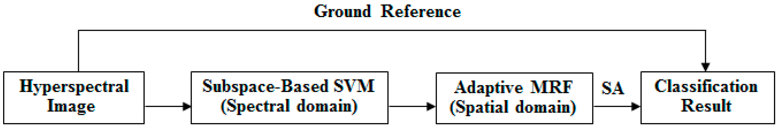
In previous work, subspace projection and MRFs have proven to be two useful methods of enhancing classification accuracy based on the spectral and spatial domains separately. Therefore, MLRsub-MRF demonstrates promising performance in hyperspectral image classification. To achieve further accuracy improvement, we wish to optimize the features from the spectral and spatial domains simultaneously. To this end, this paper proposes two new algorithms that combine SVMsub with an adaptive MRF approach (eMRF or aMRF). This section introduces the proposed methods, which belong to a framework that is divided into three components. In the spectral domain, the subspace projection technique is combined with an SVM classifier, in the procedure that we call SVMsub, to reduce the dimensionality and thereby circumvent the problems of the Hughes phenomenon and mixed pixels. In the spatial domain, two adaptive MRF algorithms are considered to optimize the spectral term, characterize the spatial information and obtain stable results via SA. The general framework of the final methods, which we call SVMsub-eMRF and SVMsub-aMRF, is illustrated in Figure 1.

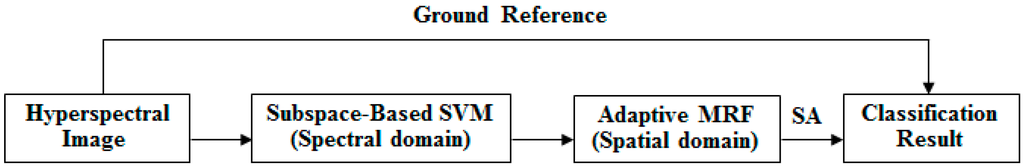
Figure 1. General framework of the proposed methods.

3.1. SVMsub

As shown in Figure 2, the basic assumption of the subspace projection method is that the samples of each class can be transformed to a lower-dimensional subspace spanned by a set of basis vectors [16]. In general, the SVMsub model is actually a novel form of an SVM nonlinear function. Under the linear mixture model assumption and the projection principle [31,32], the within-class autocorrelation matrix is first used to calculate the eigenvalues and the eigenvector matrix, which is used as the transformation matrix. Then, the class-dependent nonlinear function constructed from the transformation matrix and the original samples are defined to obtain the projected samples. Finally, these projected samples are used as the new training data for the SVM classifier to evaluate the results of the SVMsub model.

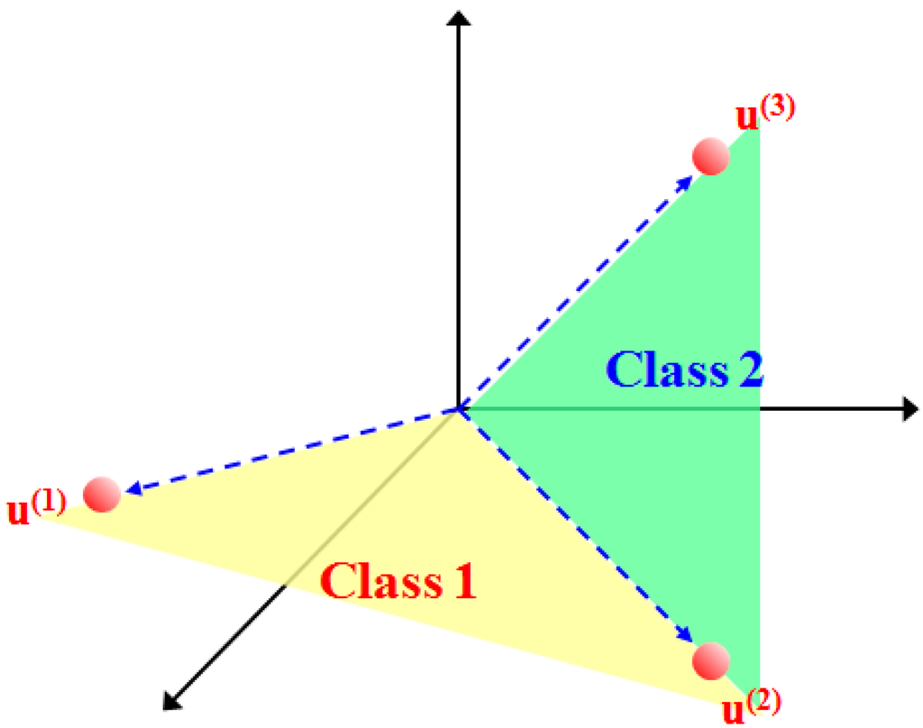
Figure 2. Illustration of subspace projection under the linear mixture model assumption, where $\{u^{(1)},u^{(2)},u^{(3)}\}$ denote the spectral endmembers. The colored spaces are the class-dependent subspaces spanned by $\{u^{(1)},u^{(2)},u^{(3)}\}$.

Under the linear mixture model assumption, for any pixel $i$, we can write

$$x_i={\displaystyle \sum _{k=1}^K{U}^{(k)}{z}_i{}^{(k)}+n_i}$$

(7)

where $n_i$ is the noise, $U^{(k)}=\{u_1^{(k)},\dots ,u_{r^{(k)}}^{(k)}\}$ is a set of $r^{(k)}$-dimensional orthonormal basis vectors for the subspaces associated with the classes $k=1,2,\dots ,K$, and $z_i^{(k)}$ represents the coordinates of $x_i$ with respect to the basis $U^{(k)}$. Let $D_l=\{D_{l^{(1)}}^{(1)},......D_{l^{(\mathrm{K})}}^{(\mathrm{K})}\}$ be the set of labeled samples, with size $l={\displaystyle \sum _{k=1}^K{l}^{(k)}}$; let $R^{(k)}=E\{x_{l^{(k)}}^{(k)}{x}_{l^{(k)}}^{(k)}{}^T\}$ denote the within-class autocorrelation matrix of class $k$; and let $x_{l^{(k)}}^{(k)}$ denote the training set of class $k$, with $l^{(k)}$ samples. By computing the eigendecomposition of $R^{(k)}$, we obtain

$$R^{(k)}=E^{(k)}{\Lambda }^{(k)}{E}^{(k)}{}^T$$

(8)

where $E^{(k)}=\{e_1^{(k)},\dots e_d^{(k)}\}$ is the eigenvector matrix and $\Lambda =diag({\lambda }_1^{(k)},\dots ,{\lambda }_d^{(k)})$ is the matrix of the eigenvalues in order of decreasing magnitude, i.e., ${\lambda }_1^{(k)}\ge \dots \ge {\lambda }_d^{(k)}$. Following [8], we define $r^{(k)}$ to cover 99% of the original spectral information, i.e.,

$$r^{(k)}=\min \{r^{(k)}:{\displaystyle \sum _{i=1}^{r^{(k)}}{\lambda }_i^{(k)}\ge }{\displaystyle \sum _{i=1}^d{\lambda }_i^{(k)}}\times 99\%\}$$

(9)

where $r^{(k)}<d$, and we take $U^{(k)}=\{e_1^{(k)},\dots e_{r^{(k)}}^{(k)}\}$ as an estimate of the class-independent $r^{(k)}$-dimensional subspace. Thus, a nonlinear function defined as

$$\varphi (x_i)={[{\Vert x_i\Vert }^2,{\Vert x_i^T{U}^{(1)}\Vert }^2,\dots ,{\Vert x_i^T{U}^{(\mathrm{K})}\Vert }^2]}^T$$

(10)

is used to obtain the projected samples

$$\varphi (x)=\{\varphi (x_1),\dots ,\varphi (x_n)\}$$

(11)

Finally, these projected samples are used as new training data for the SVM classifier to evaluate the results of the SVMsub model.

$$y_i=f(\varphi (x_i))=\mathrm{sgn}\left({\displaystyle \sum _{i=1}^l{y}_i{\alpha }_i(\varphi {(x_i)}^T\cdot \varphi (x))+b}\right)$$

(12)

where $0\le {\alpha }_i\le C$, with $C$ being the soft margin parameter. As shown in Equation (12), the projected samples that are used as the input data in our approach are approximately $K$-dimensional, independent of the size of the training set. Thus, this constitutes a significant advantage of our method compared with certain conventional kernel methods, such as those based on Gaussian or polynomial radial basis functions (RBFs) [33,34]. The pseudocode for the subspace-based SVM algorithm, abbreviated as SVMsub, is shown in Algorithm 1.

Algorithm 1 SVMsub

Input: The available training data $X={\{x_i\}}_{i=1}^l$, their class labels ${\omega }_i$, and the test sample set with class labels represented by $y$.

for $k=1$ to $K$ do

$U^{(k)}\equiv \mathsf{\Psi }(x_{l^{(k)}}^k)$ ($\ast$ $\mathsf{\Psi }$ computes the subspace according to Equations (7)–(9) $\ast$)

end

for $i=1$ to $l$ do

$\varphi (x_i)\equiv \mathrm{{\rm Z}}(x_i)$ ($\ast$ $\mathrm{{\rm Z}}$ computes the projected samples according to Equations (10) and (11) $\ast$)

end

for $i=1$ to $n$ do

$y_i=\mathrm{\Upsilon }(\varphi (x_i))$ ($\ast$ $\mathrm{\Upsilon }$ computes the SVM results according to Equation (12) $\ast$)

end

Output: The class labels $y$.

3.2. SVMsub-eMRF

Based on the results of SVMsub and the improved version of Platt’s posterior probability [35,36], the posterior probability distribution of the classified pixels is given by

$$p({\omega }_k|\varphi (x_i))=-\ln (1+\exp [Af(\varphi (x_i))+B])$$

(13)

where $A$ and $B$ are the function parameters obtained by minimizing the cross-entropy error function. Thus, the classic MRF model based on SVMsub can be expressed as follows:

$$p(x_i)=-\ln (1+\exp [Af(\varphi (x_i))+B])-\beta {\displaystyle \sum _{\partial i}[1-\delta ({\omega }_{ki},}{\omega }_{\partial i})]$$

(14)

In this paper, we multiply $p(x_i)$ by $(-1)$ to construct the initial energy function [37] for the subsequent SA. Thus, a Maximum A Posteriori (MAP) problem is converted into an energy minimization problem, and the energy function of SVMsub-MRF can be written as follows:

$$E(x_i)=\ln (1+\exp [Af(\varphi (x_i))+B])+\beta {\displaystyle \sum _{\partial i}[1-\delta ({\omega }_{ki},}{\omega }_{\partial i})]$$

(15)

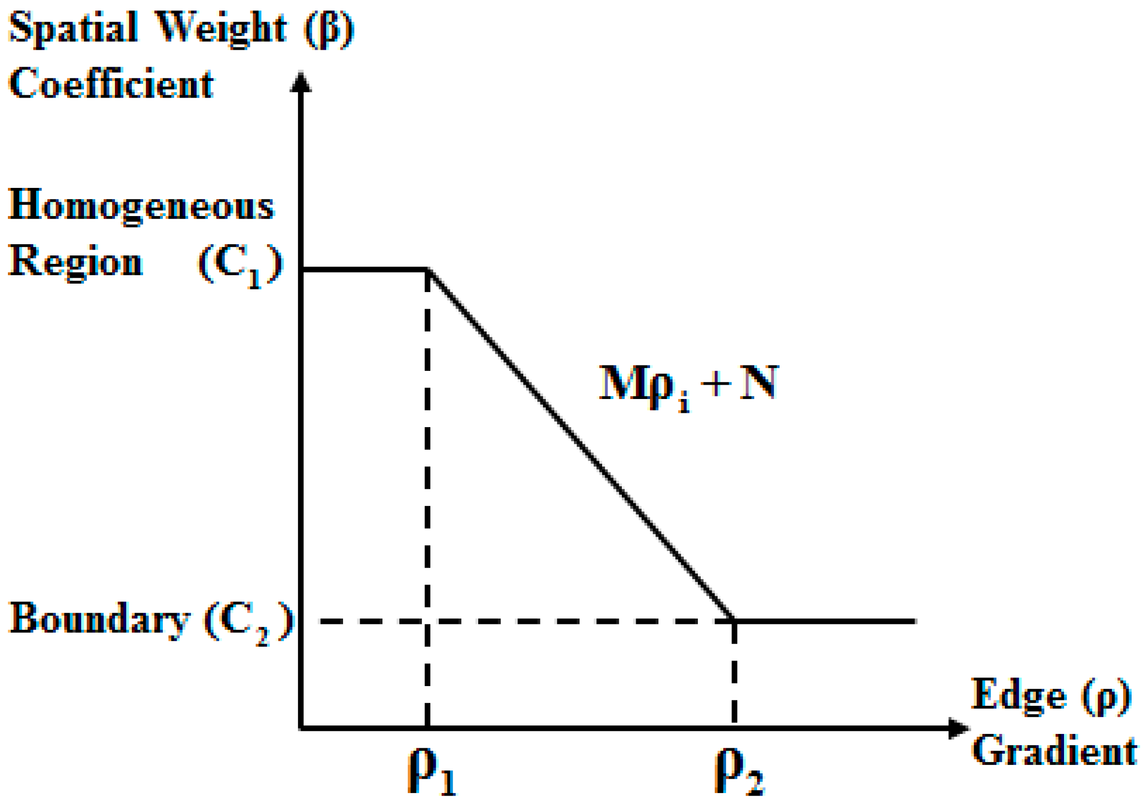
For the replacement of the global spatial weight coefficient $\beta$ with the local spatial weight coefficients ${\beta }_i$, the eMRF algorithm first uses the minimum noise fraction (MNF) transform [38] to obtain the first principal component for edge detection using a detector such as the Canny detector or the Laplacian of Gaussian (LoG) detector [39]. Based on the edge detection results, the eMRF algorithm considers two thresholds, ${\rho }_1$ and ${\rho }_2$, for identifying edges, where ${\rho }_1<{\rho }_2$. As shown in Figure 3, when the gradient of pixel $i$ is higher than ${\rho }_2$, it can be concluded that pixel $i$ is located on a boundary. By contrast, pixel $i$ is located in a homogeneous region when its gradient is lower than ${\rho }_1$.

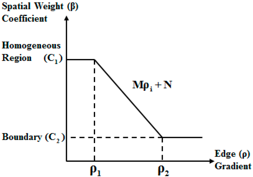
Figure 3. Relationship between the weighting coefficient and the combined edge gradient.

According to the relationship between the spatial weight coefficient of a pixel and its spatial location, we have

$${\beta }_i=\{\begin{array}{cc}{C}_1& {\rho }_i\le {\rho }_1\\ M{\rho }_i+N& {\rho }_1<{\rho }_i<{\rho }_2\\ C_2& {\rho }_i\ge {\rho }_2\end{array}$$

(16)

where ${\rho }_i$ is the gradient of pixel $i$ and $C_1$ and $C_2$ ($C_1>C_2$) are the constants that define the best values of the spatial weight coefficient for a pixel in a homogeneous region and for a pixel on a boundary, respectively. Furthermore, $M$ and $N$ are function parameters that can be calculated based on the boundary thresholds:

$$M=\frac{C_2-C_1}{{\rho }_2-{\rho }_1}，N=\frac{C_1{\rho }_2-C_2{\rho }_1}{{\rho }_2-{\rho }_1}$$

(17)

After the normalization to obtain ${\beta }_{eMRF}$, the energy function of SVMsub-eMRF is finally given by

$$\mathrm{E}{(x_i)}_{eMRF}=\ln (1+\exp [Af(\varphi (x_i))+B])+{\beta }_{eMRF}{\displaystyle \sum _{\partial i}[1-\delta ({\omega }_{ki},}{\omega }_{\partial i})].$$

(18)

The pseudocode for the subspace-based SVM algorithm combined with the edge-constrained MRF algorithm, abbreviated as SVMsub-eMRF, is shown in Algorithm 2.

Algorithm 2 SVMsub-eMRF

Input: The available training data $X={\{x_i\}}_{i=1}^l$, their class labels ${\omega }_i$, and the test sample set with class labels represented by $y$.

Step 1: Compute the results of SVMsub according to Algorithm 1;

Step 2: Obtain the first principal component using the MNF transform;

Step 3: Detect the edges using the Canny or LoG detector and the results of Step 2;

Step 4: Define the thresholds ${\rho }_1$ and ${\rho }_2$ to determine the ${\beta }_i$ using the results of Step 3 according to Equations (16) and (17);

Step 5: Determine the final class labels $y$ according to Equation (18);

Output: The class labels $y$.

3.3. SVMsub-aMRF

To obtain the local spatial weight coefficients ${\beta }_i$, the RHI can also be used to estimate the local spatial variations. The aMRF model first uses the noise-adjusted principal components (NAPC) transform to obtain the first principal component to calculate the RHI:

$$RH{I}_i=\frac{{\mathrm{var}}_k}{{\mathrm{var}}_i}$$

(19)

where ${\mathrm{var}}_k$ represents the class-decision variance of the neighborhood of pixel $i$ as determined by majority voting rules and ${\mathrm{var}}_i$ is the local variance of pixel $i$ [40]. When $RH{I}_i$ is high, it can be concluded that pixel $i$ is located in a homogeneous region. By contrast, pixel $i$ is on a boundary when $RH{I}_i$ is low. Therefore, the local spatial weight coefficient ${\beta }_i$ can be defined as follows:

$${\beta }_i={\beta }_{0}RH{I}_i={\beta }_0\frac{{\mathrm{var}}_k}{{\mathrm{var}}_i}$$

(20)

where ${\beta }_0$ is the spatial weight coefficient when ${\mathrm{var}}_i={\mathrm{var}}_k$; usually, ${\beta }_0=1$. For integration with the spectral term, it also necessary to normalize the spatial weight coefficients, i.e., ${\beta }_{aMRF}=\frac{{\beta }_i}{n}$, where $n$ is the number of pixels in the neighborhood. Thus, the SVMsub-aMRF model is finally given by

$$p(x_i)=a_i(k)+{\beta }_{aMRF}{b}_i(k)$$

(21)

and the energy function is expressed as

$$\mathrm{E}{(x_i)}_{aMRF}=\ln (1+\exp [Af(\varphi (x_i))+B])+{\beta }_{aMRF}{\displaystyle \sum _{\partial i}[1-\delta ({\omega }_{ki},}{\omega }_{\partial i})].$$

(22)

The pseudocode for the subspace-based SVM algorithm combined with the RHI-based aMRF algorithm, abbreviated as SVMsub-aMRF, is shown in Algorithm 3.

Algorithm 3 SVMsub-aMRF

Input: The available training data $X={\{x_i\}}_{i=1}^l$, their class labels ${\omega }_i$, and the test sample set with class labels represented by $y$.

Step 1: Compute the results of SVMsub according to Algorithm 1;

Step 2: Obtain the first principal component using the NAPC transform;

Step 3: Calculate the RHIs using the result of Step 1 and Step 2 according to Equation (19);

Step 4: Compute the ${\beta }_i$ using the results of Step 3 according to Equation (20);

Step 5: Determine the final class labels $y$ according to Equations (21) and (22);

Output: The class labels $y$.

4. Experiments

In this section, we evaluate the performance of the proposed SVMsub-eMRF and SVMsub-aMRF algorithms using two widely used hyperspectral data sets, one collected by AVIRIS over the Indian Pines region in Indiana and the other collected by ROSIS over the University of Pavia in Italy. The land-cover types in the Indian Pines region mainly consist of vegetation and crops. By contrast, the University of Pavia landscape is more urban, with several artificial geographical objects. For comparative purposes, we also consider several other supervised classifiers, such as MLRsub [10], MLRsub-MRF [16], SVM [3] and SVM-MRF [41], which are well-established techniques in the domain of spectral and spectral-spatial hyperspectral image classification. To ensure the fairness of the comparison of these methods, we use the overall accuracy (OA), the κ statistic, the individual accuracies and the computation time to evaluate the results of the different methods. Moreover, we set the same threshold parameters to control the loss of spectral information after the subspace projection of the data for MLRsub and SVMsub. Furthermore, we consider the same initial global spatial weight for the different MRF-based methods.

It should be noted that all spectral-spatial models considered in our experiments are optimized using the SA algorithm, which is a common method of minimizing the global energy of MRFs [42]. The Metropolis criterion and cooling schedule were used to control the behavior of the algorithm in obtaining the approximate global optimal solution. The pseudocode of the SA algorithm is presented in Algorithm 4.

Algorithm 4 SA Optimization

Input: The available training data $X={\{x_i\}}_{i=1}^n$, their class labels ${\omega }_i$, and a lowest temperature $t$.

Step 1: Obtain the initial energy function $\mathrm{E}(x_i)$ according to the results of SVMsub-eMRF or SVMsub-aMRF;

Step 2: Randomly vary the classes and calculate a new energy function ${\mathrm{E}}^{’}(x_i)$;

Step 3: Compute the difference between the results of Step 1 and Step 2: $\Delta \mathrm{E}={\mathrm{E}}^{’}(x_i)-\mathrm{E}(x_i)$;

Step 4: If $\Delta \mathrm{E}<0$, replace the class labels with the current ones. Otherwise, leave them unchanged;

Step 5: Return to Step 2 until the predefined lowest temperature $t$ has been reached;

Step 6: Determine the final class labels $y$;

Output: The class labels $y$.

4.1. Experiments Using the AVIRIS Indian Pines Data Set

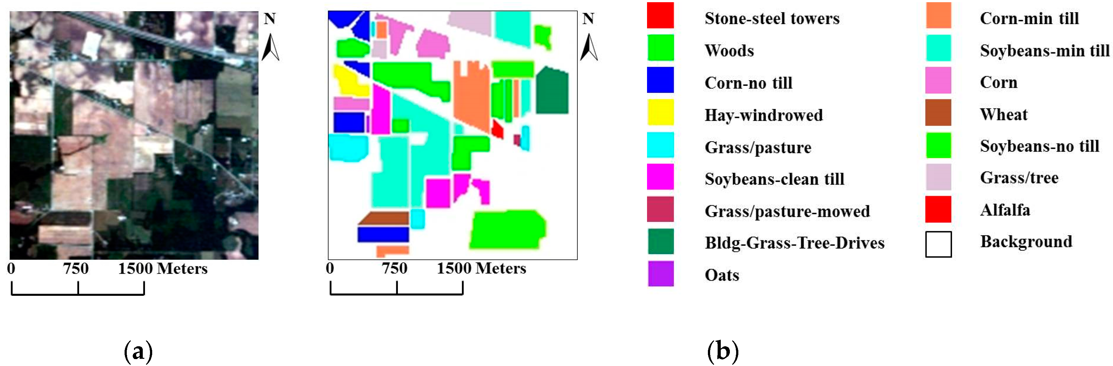
For our first experiment, we used the well-known AVIRIS Indian Pines data set, which was collected over northwestern Indiana in June of 1992, to compare the proposed models with other methods. The scene contains $145\times 145$ pixels, with 220 spectral bands in the spectral range from 0.4 $\mathsf{\mu }\mathrm{m}$ to 2.5 $\mathsf{\mu }\mathrm{m}$ and a nominal spectral resolution of 10 $\mathrm{nm}$. The ground reference data contain a total of 10,366 samples belonging to 16 mutually exclusive classes. Figure 4a shows a true-color composite of the image, whereas Figure 4b shows the 16 ground reference object classes.

Figure 4. (a) True-color composite of the Airborne Visible/Infrared Imaging Spectrometer (AVIRIS) Indian Pines scene; (b) Ground reference map containing 16 mutually exclusive land-cover classes.

In our first two tests, we used two versions of the Indian Pines data, one with all 220 spectral bands available and the other with only 200 channels after the removal of 20 bands due to noise and water absorption, to evaluate the performances of the compared methods under different noise conditions. Specifically, for these tests, 30 samples per class were randomly selected to obtain a total of 480 training samples, which is a very limited training sample size (approximately 2.3% of the total). Table 1 and Table 2 report the results for the two scenarios in terms of the OAs, κ statistic values and individual accuracies after twenty Monte Carlo runs. For this comparison, we defined $r^{(k)}$ to cover 99% of ${\displaystyle \sum _{i=1}^d{\lambda }_i^{(k)}}$ and set the initial global weight coefficient $\beta$ to 4.0.

Table 1. Overall and average class accuracies and κ statistic values obtained for the Airborne Visible/Infrared Imaging Spectrometer (AVIRIS) Indian Pines data set using 220 spectral bands and a training sample size of 30 samples per class. The best results are highlighted in bold typeface.

Class	Samp-les	Spectral Space			Spectral-Spatial Space
		SVM	MLRsub	SVMsub	SVM-MRF	MLRsub-MRF	MLRsub-aMRF	SVMsub-MRF	SVMsub-eMRF	SVMsub-aMRF
Alfalfa	54	78.75%	85.83%	87.92%	100.00%	98.15%	98.15%	98.15%	98.15%	98.15%
Corn-no till	1434	40.44%	64.22%	67.73%	59.27%	86.12%	91.21%	83.40%	83.33%	84.59%
Corn-min till	834	43.21%	60.99%	67.71%	59.95%	70.74%	84.53%	77.58%	83.21%	80.22%
Corn	234	66.39%	77.60%	86.14%	99.57%	99.57%	97.86%	100.00%	98.72%	100.00%
Grass/pasture	497	75.22%	84.07%	87.47%	89.54%	93.36%	91.55%	92.56%	94.77%	95.98%
Grass/tree	747	77.26%	91.82%	92.80%	99.33%	97.99%	98.39%	97.59%	97.59%	97.99%
Grass/pasture-mowed	26	84.62%	86.15%	87.69%	92.31%	100.00%	92.31%	84.62%	92.31%	96.15%
Hay-windrowed	489	81.15%	95.46%	96.52%	79.75%	99.39%	99.18%	99.18%	98.77%	98.57%
Oats	20	71.00%	94.00%	82.00%	100.00%	100.00%	100.00%	100.00%	90.00%	100.00%
Soybeans-no till	968	51.93%	61.46%	66.88%	76.65%	95.66%	91.53%	93.08%	95.66%	96.69%
Soybeans-min till	2468	52.78%	44.33%	72.16%	64.02%	65.36%	65.36%	84.08%	85.53%	87.60%
Soybeans-clean till	614	50.38%	67.84%	82.35%	72.64%	88.60%	93.97%	95.44%	95.28%	99.19%
Wheat	212	93.25%	99.56%	99.23%	99.53%	100.00%	99.06%	99.53%	99.53%	100.00%
Woods	1294	75.89%	95.59%	90.27%	94.67%	99.15%	99.38%	94.28%	94.74%	96.60%
Bldg-Grass-Tree-Drives	380	50.65%	36.46%	68.87%	77.63%	56.84%	52.37%	90.79%	88.68%	80.79%
Stone-steel towers	95	96.30%	90.73%	91.51%	96.84%	100.00%	100.00%	97.89%	98.95%	97.89%
Overall accuracy $\kappa$ statistic		58.47%	67.62%	77.78%	75.72%	84.20%	85.66%	89.49%	90.57%	91.22%
		0.53	0.64	0.75	0.73	0.82	0.84	0.88	0.89	0.90

Table 2. Overall and average class accuracies and κ statistic values obtained for the AVIRIS Indian Pines data set using 200 spectral bands and a training sample size of 30 samples per class. The best results are highlighted in bold typeface.

Class	Samp-les	Spectral Space			Spectral-Spatial Space
		SVM	MLRsub	SVMsub	SVM-MRF	MLRsub-MRF	MLRsub-aMRF	SVMsub-MRF	SVMsub-eMRF	SVMsub-aMRF
Alfalfa	54	91.59%	78.99%	89.89%	98.15%	98.15%	98.15%	94.44%	96.30%	96.30%
Corn-no till	1434	55.82%	56.85%	66.84%	60.11%	68.34%	67.99%	72.87%	72.52%	75.45%
Corn-min till	834	58.60%	61.22%	72.21%	76.98%	80.22%	83.69%	85.73%	90.41%	91.13%
Corn	234	76.98%	70.74%	86.53%	97.44%	94.87%	97.01%	99.57%	97.44%	98.72%
Grass/pasture	497	86.64%	84.75%	89.86%	93.76%	95.17%	97.18%	90.34%	93.36%	95.77%
Grass/tree	747	85.92%	90.43%	94.85%	93.71%	98.13%	99.33%	98.80%	99.06%	99.20%
Grass/pasture-mowed	26	92.31%	90.77%	90.77%	100.00%	100.00%	100.00%	96.15%	100.00%	100.00%
Hay-windrowed	489	92.28%	95.48%	96.14%	98.77%	99.18%	99.18%	99.18%	98.16%	98.57%
Oats	20	88.00%	88.00%	86.00%	100.00%	100.00%	100.00%	50.00%	100.00%	90.00%
Soybeans-no till	968	69.47%	59.26%	72.70%	77.38%	79.75%	87.29%	90.08%	91.43%	88.02%
Soybeans-min till	2468	65.35%	44.70%	67.50%	85.78%	62.60%	64.14%	77.19%	77.39%	78.73%
Soybeans-clean till	614	62.85%	66.76%	82.20%	83.22%	74.92%	69.06%	96.25%	94.46%	98.21%
Wheat	212	95.91%	99.45%	99.45%	100.00%	99.53%	99.53%	100.00%	99.53%	99.53%
Woods	1294	85.98%	85.28%	91.38%	89.10%	97.76%	96.06%	98.22%	97.53%	97.84%
Bldg-Grass-Tree-Drives	380	60.62%	45.39%	61.71%	83.95%	61.05%	71.84%	67.11%	76.05%	76.32%
Stone-steel towers	95	96.28%	91.32%	91.01%	100.00%	100.00%	100.00%	97.89%	98.95%	98.95%
Overall accuracy $\kappa$ statistic		71.01%	65.19%	77.56%	83.31%	79.51%	80.87%	86.34%	87.16%	88.04%
		0.67	0.61	0.75	0.81	0.77	0.78	0.85	0.86	0.86

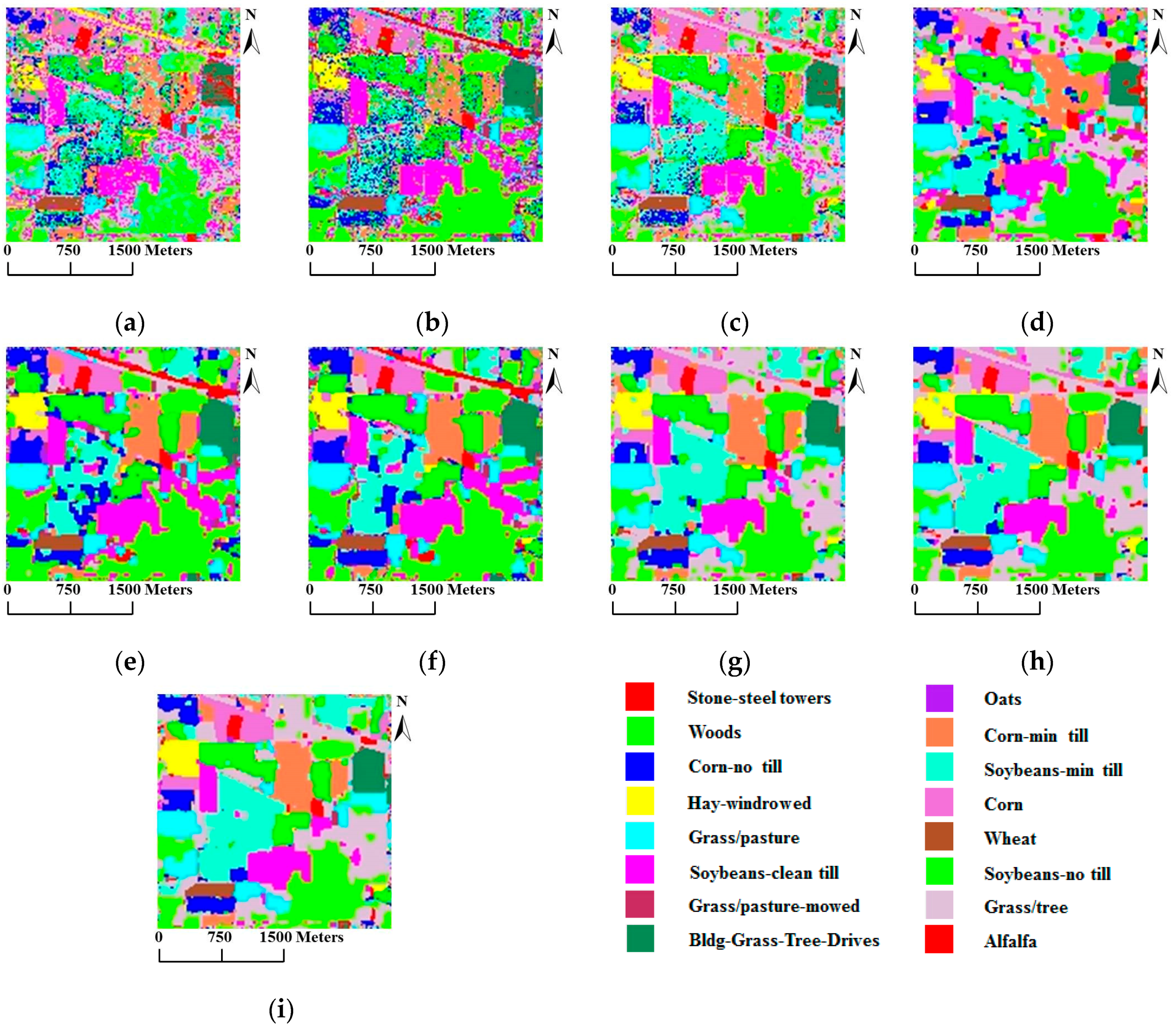
From these two tables, we can make the following observations: (1) SVMsub achieves the best results when only information from the spectral domain is used, thereby demonstrating the advantages of the subspace projection technique combined with the SVM classifier; (2) SVM-MRF yields higher accuracies than SVM, providing further evidence that the integration of spatial and spectral information via the MRF approach helps to improve the classification accuracy; (3) SVMsub-MRF achieves better results compared with SVMsub and SVM-MRF, which serves as further proof of the effectiveness of combining the subspace projection technique with the MRF approach. The same can be said of the results obtained by MLRsub-MRF and MLRsub; (4) SVMsub-aMRF yields the best accuracies compared with SVMsub-eMRF and SVMsub-MRF, thereby demonstrating that the adaptive technique is a powerful means of improving the classification accuracy; (5) SVMsub-aMRF achieves superior results compared with MLRsub-aMRF, thereby proving the effectiveness and robustness of the proposed method. In general, SVMsub-eMRF achieves excellent accuracies, with OAs of 90.57% and 87.16%. SVMsub-aMRF achieves the best accuracies in both scenarios, with OAs of 91.22% and 88.04%, respectively. Notably, the average individual accuracies of SVMsub-aMRF and SVMsub-eMRF are also generally superior to those of the other methods. Figure 5 shows the classification and segmentation maps produced by the methods listed in Table 1.

Figure 5. Classification/segmentation maps produced by the various tested methods for the AVIRIS Indian Pines scene (overall accuracies are reported in parentheses). (a) SVM (58.47%); (b) MLRsub (67.62%); (c) SVMsub (77.78%); (d) SVM-MRF (75.72%); (e) MLRsub-MRF (84.20%); (f) MLRsub-aMRF (85.66%); (g) SVMsub-MRF (89.49%); (h) SVMsub-eMRF (90.57%); (i) SVMsub-aMRF (91.22%).

In our second test using the AVIRIS Indian Pines data set, we analyzed the performances of our methods compared with those of other spectral-spatial classifiers using different numbers of samples. To evaluate the sensitivity to the number of samples, we generated the training sets by randomly selecting 10, 15, 20, 25, 30, 35, 40, 45 and 50 labeled samples per class. Table 3 reports the obtained values of the OA, the κ statistic and the computational cost, including both training and testing times. This comparison yields similar conclusions to those drawn from the first two tests presented above: (1) SVMsub-MRF achieves better results than SVM-MRF (by approximately 10% in each group); (2) SVMsub-aMRF yields higher accuracies compared with SVMsub-eMRF and SVMsub-MRF. Additionally, MLRsub-aMRF performs better than MLRsub-MRF; (3) SVMsub-aMRF yields the best accuracies among all methods in each group; for example, this method achieves an OA of 93.03% and a $\kappa$ value of 0.92 in the group corresponding to 900 labeled samples (approximately 50 samples per class). This experiment again proves that our proposed method is robust and reliable. In addition, it should be noted that the computational costs of the models integrated with a subspace projection method are generally less than those of the other methods, even when a large number of training samples are used. Figure 6 shows the OA results obtained by the various methods as a function of the number of labeled samples per class.

Table 3. Overall classification accuracies (in percent) and κ statistic values obtained by the various tested methods for the AVIRIS Indian Pines scene using different numbers of training samples. The computational costs (in parentheses) are also presented. Both the total number of samples used and the (approximate) number of training samples per class (in parentheses) are shown.

Samples (per Class)	Classification Method
		SVM-MRF	MLRsub-MRF	MLRsub-aMRF	SVMsub-MRF	SVMsub-eMRF	SVMsub-aMRF
160 (10)	OA (Time)	44.56% (2.83)	65.58% (2.70)	66.52% (2.71)	63.70% (0.89)	68.10% (0.99)	69.98% (0.89)
	$\kappa$ statistic	0.3847	0.6188	0.6296	0.6000	0.6457	0.6667
240 (15)	OA (Time)	47.19% (3.60)	77.32% (3.23)	79.49% (3.23)	75.21% (0.93)	78.92% (1.03)	79.90% (0.94)
	$\kappa$ statistic	0.4208	0.7430	0.7670	0.7217	0.7635	0.7736
320 (20)	OA (Time)	65.28% (4.56)	79.15% (3.43)	80.95% (3.43)	81.74% (0.95)	83.35% (1.05)	84.14% (0.96)
	$\kappa$ statistic	0.6098	0.7628	0.7802	0.7921	0.8104	0.8193
400 (25)	OA (Time)	69.47% (5.68)	81.64% (3.46)	82.94% (3.47)	84.03% (0.97)	86.49% (1.07)	87.02% (0.97)
	$\kappa$ statistic	0.6551	0.7908	0.8068	0.8186	0.8441	0.8517
480 (30)	OA (Time)	75.72% (6.94)	84.20% (3.66)	85.66% (3.68)	89.49% (0.99)	90.57% (1.09)	91.22% (1.00)
	$\kappa$ statistic	0.7274	0.8219	0.8387	0.8809	0.8931	0.9003
560 (35)	OA (Time)	75.75% (8.23)	84.42% (3.98)	88.18% (3.99)	86.63% (1.01)	89.54% (1.12)	90.23% (1.02)
	$\kappa$ statistic	0.7281	0.8237	0.8658	0.8525	0.8815	0.8909
640 (40)	OA (Time)	79.73% (9.73)	86.86% (4.06)	88.90% (4.07)	91.55% (1.05)	91.63% (1.16)	92.20% (1.05)
	$\kappa$ statistic	0.7701	0.8488	0.8724	0.9037	0.9046	0.9110
720 (45)	OA (Time)	80.47% (11.69)	88.35% (4.38)	90.34% (4.39)	90.54% (1.07)	91.57% (1.18)	91.61% (1.08)
	$\kappa$ statistic	0.7787	0.8670	0.8898	0.8922	0.9040	0.9046
800 (50)	OA (Time)	83.79% (14.40)	88.74% (4.64)	90.83% (4.65)	91.28% (1.12)	91.94% (1.22)	93.03% (1.13)
	$\kappa$ statistic	0.8164	0.8708	0.8957	0.9011	0.9088	0.9195

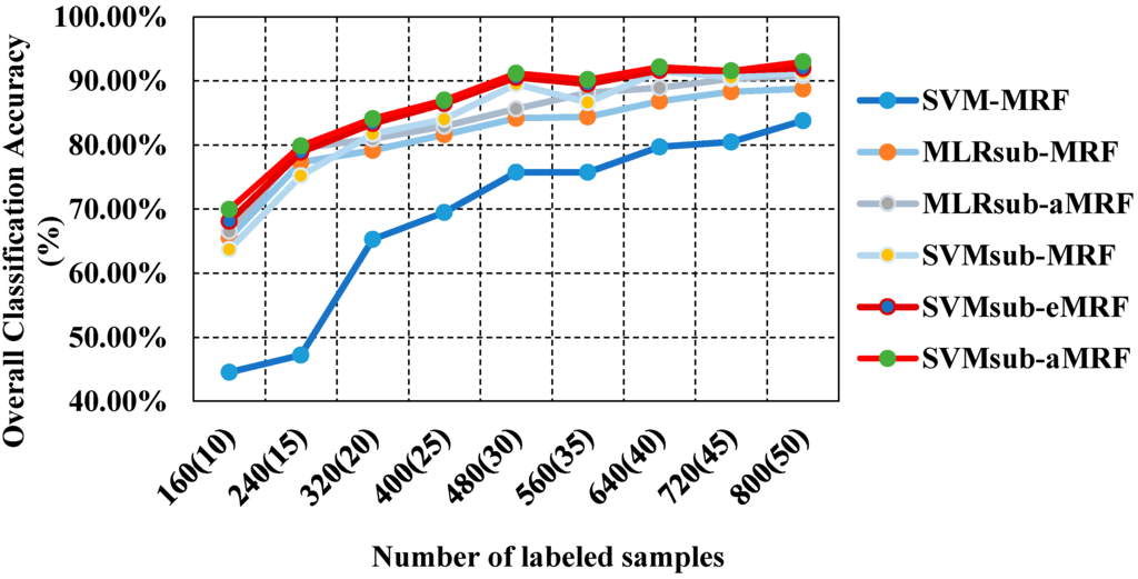
Figure 6. Overall accuracy results as a function of the number of labeled samples for the Indian Pines data set.

4.2. Experiments Using the ROSIS University of Pavia Data Set

In our second experiment, we used the real hyperspectral data set collected in 2001 by ROSIS over the University of Pavia in Italy. The ROSIS optical sensor provides up to 115 bands with a spectral range coverage ranging from 0.43 µm to 0.86 µm. The size of the University of Pavia image is 610 × 340 pixels, with 103 spectral bands after the removal of 12 bands of noise and water absorption. The ground reference data contain a total of 3921 training samples and 42,776 test samples belonging to nine classes. Figure 7a shows a true-color composite of the image, whereas Figure 7b shows the nine ground reference classes corresponding to the detailed features in the image.

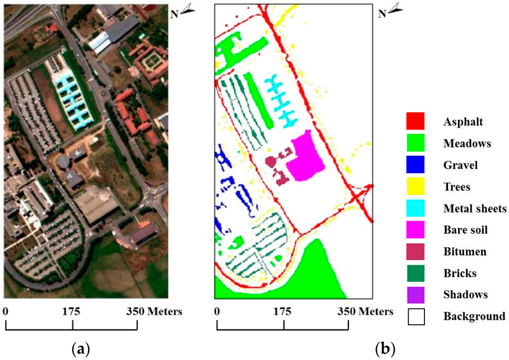
Figure 7. (a) True-color composite of the Reflective Optics Spectrographic Imaging System (ROSIS) Pavia scene; (b) Ground reference map containing nine mutually exclusive land-cover classes.

In our first test using the University of Pavia data set, we used 20 training samples per class, for a total of 180 training samples, which is a relatively small number. Table 4 reports the OA, κ statistic and individual accuracy results after twenty Monte Carlo runs. For this comparison, we again defined $r^{(k)}$ to cover 99% of ${\displaystyle \sum _{i=1}^d{\lambda }_i^{(k)}}$ and set the global weight coefficient $\beta$ to 4.0. From the results, we obtain very similar conclusions to those obtained using the AVIRIS Indian Pines data set: (1) SVMsub achieves the best accuracy compared with SVM and MLRsub, with an OA of 71.38%; (2) SVMsub-eMRF provides a considerable improvement, with an OA of 79.84%, whereas SVMsub-aMRF yields the best accuracy in the spectral-spatial domain, with an OA of 81.94%. Likewise, the average individual accuracies of SVMsub-aMRF and SVMsub-eMRF are generally higher than those of the other approaches. Figure 8 shows the classification and segmentation maps produced by the aforementioned methods.

Table 4. Overall, average, and individual class accuracies (in percent) and κ statistic values obtained for the Reflective Optics Spectrographic Imaging System (ROSIS) University of Pavia data set with a training sample size of 20 samples per class. The best results are highlighted in bold typeface.

Class	Samples		Spectral Space			Spectral-Spatial Space
	Train	Test	SVM	MLR-sub	SVM-sub	SVM-MRF	MLRsub-MRF	MLRsub-aMRF	SVMsub-MRF	SVMsub-eMRF	SVMsub-aMRF
Alfalfa	540	6631	63.64%	43.01%	63.52%	76.05%	66.75%	73.15%	70.96%	73.16%	83.60%
Bare soil	548	18,649	57.86%	71.11%	61.82%	60.19%	69.25%	69.90%	68.61%	69.13%	69.08%
Bitumen	392	2099	82.28%	62.12%	85.99%	88.49%	44.27%	37.70%	95.20%	91.84%	97.15%
Bricks	524	3064	97.00%	91.25%	96.38%	97.35%	97.06%	96.77%	96.27%	95.05%	93.60%
Gravel	265	1345	99.41%	98.66%	98.96%	99.85%	99.13%	99.78%	99.64%	98.77%	99.71%
Meadows	532	5029	72.72%	62.95%	77.49%	82.92%	77.06%	68.95%	86.93%	87.79%	90.73%
Metal sheets	375	1330	91.05%	84.51%	80.00%	97.20%	91.67%	97.27%	91.52%	91.96%	96.31%
Shadows	514	3682	80.28%	49.29%	76.10%	91.49%	68.51%	74.45%	93.37%	96.31%	94.46%
Trees	231	947	99.89%	100.00%	99.58%	99.81%	100.00%	100.00%	99.71%	99.42%	94.46%
Overall accuracy $\kappa$ statistic			69.70%	66.84%	71.38%	75.71%	72.97%	73.67%	79.20%	79.84%	81.94%
			0.63	0.58	0.65	0.70	0.66	0.67	0.74	0.75	0.78

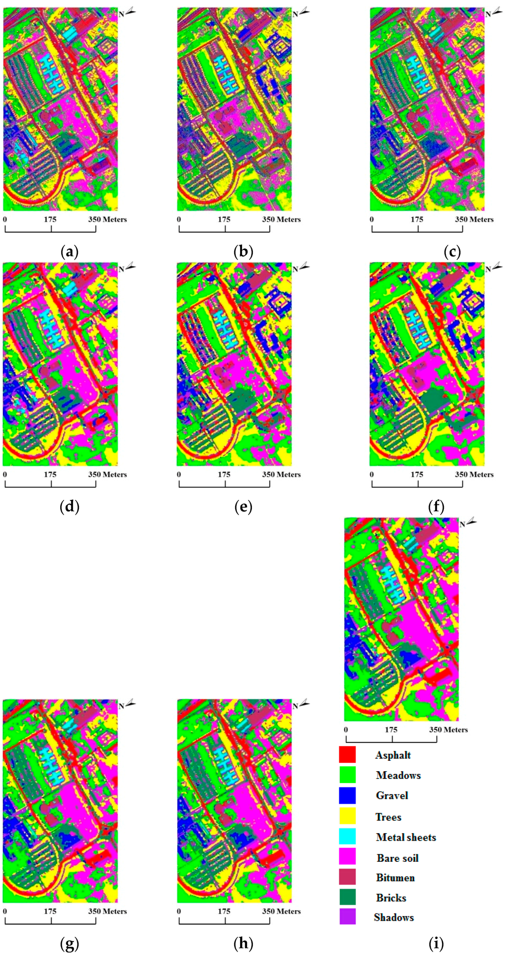
Figure 8. Classification/segmentation maps produced by the various tested methods for the ROSIS University of Pavia scene (overall accuracies are reported in parentheses). (a) SVM (69.70%); (b) MLRsub (66.84%); (c) SVMsub (71.38%); (d) SVM-MRF (75.71%); (e) MLRsub-MRF (72.97%); (f) MLRsub-aMRF (73.67%); (g) SVMsub-MRF (79.20%); (h) SVMsub-eMRF (79.84%); (i) SVMsub-aMRF (81.94%).

In our second test using the University of Pavia data set, we again analyzed the performances of the methods in the spectral-spatial domain using different numbers of training samples. We used approximately the same number of training samples per class (except for those classes that are very small) to generate a total of nine sets of training samples ranging in size from 180 to 900 samples. Table 5 reports the obtained values of the OA, the κ statistic and the computational cost. As shown in Table 5, SVMsub-aMRF yields the best accuracies compared with the other methods for each set. For instance, SVMsub-eMRF and SVMsub-aMRF achieve OAs of 92.61% and 93.50%, respectively, in the group corresponding to 900 labeled samples (approximately 35 samples per class). Figure 9 shows the OA results obtained by the various methods as a function of the number of labeled samples. Similar conclusions obtained in all cases for different types of images under different conditions further prove the effectiveness and robustness of our proposed method.

Table 5. Overall classification accuracies (in percent) and κ statistic values obtained by the various tested methods for the ROSIS University of Pavia data set scene using different numbers of training samples. The computational costs (in parentheses) are also presented. Both the total number of samples used and the (approximate) number of training samples per class (in parentheses) are shown.

Samples (per Class)	Classification Method
		SVM-MRF	MLRsub-MRF	MLRsub-aMRF	SVMsub-MRF	SVMsub-eMRF	SVMsub-aMRF
180 (20)	OA (Time)	75.71% (9.05)	72.97% (5.97)	73.67% (5.99)	79.20% (3.12)	79.84% (4.17)	81.94% (3.14)
	$\kappa$ statistic	0.7021	0.6632	0.6693	0.7415	0.7491	0.7751
270 (30)	OA (Time)	79.59% (11.34)	73.96% (6.13)	75.66% (6.16)	82.67% (3.20)	83.20% (4.25)	83.30% (3.23)
	$\kappa$ statistic	0.7496	0.6728	0.6938	0.7806	0.7875	0.7885
360 (40)	OA (Time)	80.99% (12.36)	77.82% (6.27)	80.37% (6.30)	82.68% (3.27)	82.98% (4.34)	83.23% (3.30)
	$\kappa$ statistic	0.7669	0.7143	0.7477	0.7844	0.7863	0.7909
450 (50)	OA (Time)	81.95% (13.05)	77.88% (6.39)	80.75% (6.41)	86.23% (3.33)	86.24% (4.46)	86.68% (3.41)
	$\kappa$ statistic	0.7772	0.7208	0.7513	0.8261	0.8263	0.8318
540 (60)	OA (Time)	82.14% (14.05)	78.98% (6.55)	81.12% (6.60)	86.37% (3.41)	86.57% (4.55)	87.15% (3.50)
	$\kappa$ statistic	0.7795	0.7349	0.7611	0.8280	0.8305	0.8375
630 (70)	OA (Time)	84.77% (15.30)	80.44% (6.60)	81.91% (6.64)	88.04% (3.50)	88.98% (4.68)	89.35% (3.62)
	$\kappa$ statistic	0.8105	0.746	0.7644	0.8471	0.8588	0.8636
720 (80)	OA (Time)	84.83% (16.35)	81.83% (6.73)	83.90% (6.75)	88.93% (3.61)	89.54% (4.79)	89.66% (3.71)
	$\kappa$ statistic	0.8107	0.7661	0.7926	0.8594	0.8668	0.8682
810 (90)	OA (Time)	85.94% (17.29)	82.58% (6.95)	84.12% (6.99)	90.03% (3.75)	90.35% (4.87)	90.69% (3.83)
	$\kappa$ statistic	0.8240	0.7774	0.7960	0.8723	0.8764	0.8806
900 (100)	OA (Time)	87.28% (18.76)	84.32% (7.01)	84.93% (7.03)	92.51% (3.87)	92.61% (4.99)	93.50% (3.95)
	$\kappa$ statistic	0.8400	0.7977	0.8051	0.9036	0.9048	0.9162

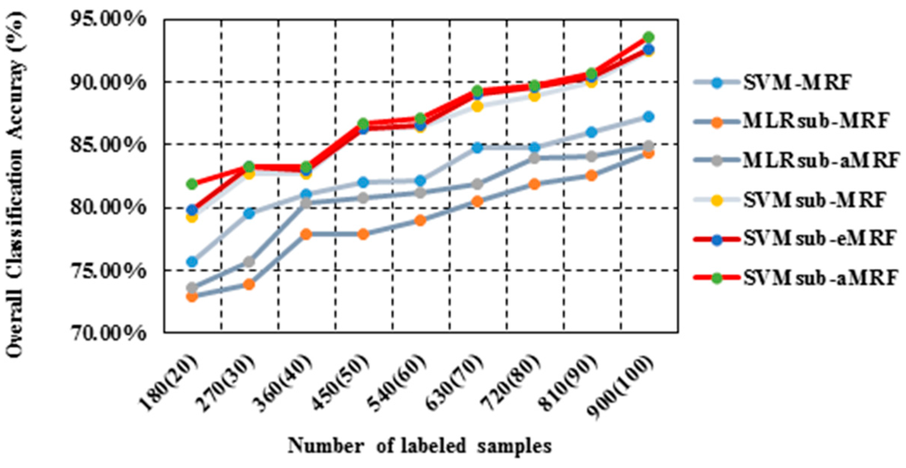
Figure 9. Overall accuracy results as a function of the number of labeled samples per class for the University of Pavia data set.

As shown in Table 5, the proposed method is insensitive to the number of training samples used. In other words, its accuracy can be guaranteed even when only a limited number of training samples are used, and the computation time will not be too high even with a large training set. We note that the number of training samples used should be adjusted depending on the application. It is suggested that a relatively large training set can be adopted for improved accuracy because the resulting increase in computation time is minimal.

5. Conclusions

The classification of hyperspectral images faces various challenges related to the Hughes phenomenon, mixed pixels, noise and so on. Several techniques have been exploited to address these problems based on data from different domains. In the spectral domain, the subspace projection algorithm has proven to be an effective method of coping with the imbalance between the high dimensionality of the data and the limited number of training samples available. In the spatial domain, the MRF approach has been shown to be a powerful technique for integrating spatial correlation information into the posterior probability distribution of the spectral features. Thus, spectral-spatial models such as MLRsub-MRF, which combine the information from these two domains, can effectively improve the classification of hyperspectral images. To obtain classification results with higher accuracy than that of MLRsub-MRF, new frameworks should allow the further, simultaneous optimization of spectral and spatial features.

In this paper, we developed two new supervised spectral-spatial hyperspectral image classification approaches called SVMsub-eMRF and SVMsub-aMRF, which integrate the subspace-based SVM classification method with an adaptive MRF approach. By projecting the original data to a class-independent subspace representation, the proposed methods use adaptive MRFs to revise the MAP results of the SVM classifier based on the projected samples, including the optimization of the final segmentation results via the SA algorithm. Experiments on two real hyperspectral data sets demonstrated that the proposed methods not only can cope with the Hughes phenomenon and the effects of noise and mixed pixels but also are able to discriminatively address the relationships exhibited by pixels in homogeneous regions or on boundaries with a low computational cost. Moreover, the classification results of the proposed methods demonstrate considerable advantages compared with those of other models. In our future work, we will focus on the application of superpixels in the existing framework and test the proposed algorithms using additional hyperspectral images.

References

- Landgrebe, D.A. Signal Theory Methods in Multispectral Remote Sensing; Wiley: New York, NY, USA, 2003. [Google Scholar]
- Qian, Y.; Yao, F.; Jia, S. Band selection for hyperspectral imagery using affinity propagation. IET Comput. Vis. 2009, 3, 213–222. [Google Scholar] [CrossRef]
- Melgani, F.; Bruzzone, L. Classification of hyperspectral remote sensing images with support vector machines. IEEE Trans. Geosci. Remote Sens. 2004, 42, 1778–1790. [Google Scholar] [CrossRef]
- Schölkopf, B.; Smola, A.J. Learning with Kernels: Support Vector Machines, Regularization, Optimization, and Beyond; MIT Press: Cambridge, MA, USA, 2002. [Google Scholar]
- Harsanyi, J.C.; Chang, C. Hyperspectral image classification and dimensionality reduction: An orthogonal subspace projection approach. IEEE Trans. Geosci. Remote Sens. 1994, 32, 779–785. [Google Scholar] [CrossRef]
- Larsen, R.; Arngren, M.; Hansen, P.W.; Nielsen, A.A. Kernel based subspace projection of near infrared hyperspectral images of maize kernels. Image Anal. 2009, 5575, 560–569. [Google Scholar]
- Chen, W.; Huang, J.; Zou, J.; Fang, B. Wavelet-face based subspace LDA method to solve small sample size problem in face recognition. Int. J. Wavelets Multiresolut. Inf. Process. 2009, 7, 199–214. [Google Scholar] [CrossRef]
- Gao, L.; Li, J.; Khodadadzadeh, M.; Plaza, A.; Zhang, B.; He, Z.; Yan, H. Subspace-based support vector machines for hyperspectral image classification. IEEE Geosci. Remote Sens. Lett. 2015, 12, 349–353. [Google Scholar]
- Li, W.; Tramel, E.W.; Prasad, S.; Fowler, J.E. Nearest regularized subspace for hyperspectral classification. IEEE Trans. Geosci. Remote Sens. 2014, 52, 477–489. [Google Scholar] [CrossRef]
- Li, J.; Bioucas-Dias, J.M.; Plaza, A. Semisupervised hyperspectral image segmentation using multinomial logistic regression with active learning. IEEE Trans. Geosci. Remote Sens. 2010, 48, 4085–4098. [Google Scholar] [CrossRef]
- Fauvel, M.; Tarabalka, Y.; Benediktsson, J.A.; Chanussot, J.; Tilton, J.C. Advances in spectral-spatial classification of hyperspectral images. Proc. IEEE 2013, 101, 652–675. [Google Scholar] [CrossRef]
- Fauvel, M.; Benediktsson, J.A.; Chanussot, J.; Sveinsson, J.R. Spectral and spatial classification of hyperspectral data using SVMs and morphological profiles. IEEE Trans. Geosci. Remote Sens. 2008, 46, 3804–3814. [Google Scholar] [CrossRef]
- Jia, S.; Xie, Y.; Tang, G.; Zhu, J. Spatial-spectral-combined sparse representation-based classification for hyperspectral imagery. Soft Comput. 2014, 1–10. [Google Scholar] [CrossRef]
- Benediktsson, J.A.; Pesaresi, M.; Arnason, K. Classification and feature extraction for remote sensing images from urban areas based on morphological transformations. IEEE Trans. Geosci. Remote Sens. 2003, 41, 1940–1949. [Google Scholar] [CrossRef]
- Benediktsson, J.A.; Palmason, J.A.; Sveinsson, J.R. Classification of hyperspectral data from urban areas based on extended morphological profiles. IEEE Trans. Geosci. Remote Sens. 2005, 43, 480–491. [Google Scholar] [CrossRef]
- Li, J.; Bioucas-Dias, J.M.; Plaza, A. Spectral-spatial hyperspectral image segmentation using subspace multinomial logistic regression and Markov random fields. IEEE Trans. Geosci. Remote Sens. 2012, 50, 809–823. [Google Scholar] [CrossRef]
- Ni, L.; Gao, L.; Li, S.; Li, J.; Zhang, B. Edge-constrained Markov random field classification by integrating hyperspectral image with LiDAR data over urban areas. J. Appl. Remote Sens. 2014, 8. [Google Scholar] [CrossRef]
- Zhang, B.; Li, S.; Jia, X.; Gao, L.; Peng, M. Adaptive Markov random field approach for classification of hyperspectral imagery. IEEE Geosci. Remote Sens. Lett. 2011, 8, 973–977. [Google Scholar] [CrossRef]
- Kirkpatrick, S.; Gelatt, C.D.; Vecchi, M.P. Optimization by simulated annealing. Science 1983, 220, 671–680. [Google Scholar] [CrossRef] [PubMed]
- Camps-Valls, G.; Bruzzone, L. Kernel-based methods for hyperspectral image classification. IEEE Trans. Geosci. Remote Sens. 2005, 43, 1351–1362. [Google Scholar] [CrossRef]
- Xie, J.; Hone, K.; Xie, W.; Gao, X.; Shi, Y.; Liu, X. Extending twin support vector machine classifier for multi-category classification problems. Intell. Data Anal. 2013, 17, 649–664. [Google Scholar]
- Vapnik, V. Statistical Learning Theory; Wiley: New York, NY, USA, 1998. [Google Scholar]
- Richards, J.A.; Jia, X. Remote Sensing Digital Image Analysis: An Introduction; Springer-Verlag: Berlin, Germany, 2006. [Google Scholar]
- Plaza, A.; Benediktsson, J.A.; Boardman, J.W.; Brazile, J.; Bruzzone, L.; Camps-Valls, G.; Chanussot, J.; Fauvel, M.; Gamba, P.; Gualtieri, A. Recent advances in techniques for hyperspectral image processing. Remote Sens. Environ. 2009, 113, S110–S122. [Google Scholar] [CrossRef]
- Zhang, Y.; Brady, M.; Smith, S. Segmentation of brain MR images through a hidden Markov random field model and the expectation-maximization algorithm. IEEE Trans. Med. Imaging 2001, 20, 45–57. [Google Scholar] [CrossRef] [PubMed]
- Geman, S.; Geman, D. Stochastic relaxation, Gibbs distributions, and the Bayesian restoration of images. IEEE Trans. Pattern Anal. Mach. Intell. 1984, 6, 721–741. [Google Scholar] [CrossRef] [PubMed]
- Jia, X.; Richards, J.A. Managing the spectral-spatial mix in context classification using Markov random fields. IEEE Geosci. Remote Sens. Lett. 2008, 5, 311–314. [Google Scholar] [CrossRef]
- Chang, C.I. Hyperspectral Imaging: Techniques for Spectral Detection and Classification; Springer Science and Business Media: New York, NY, USA, 2003. [Google Scholar]
- Zhong, Y.; Lin, X.; Zhang, L. A support vector conditional random fields classifier with a Mahalanobis distance boundary constraint for high spatial resolution remote sensing imagery. IEEE J. Sel. Top. Appl. Earth Obs. Remote Sens. 2014, 7, 1314–1330. [Google Scholar] [CrossRef]
- Jiménez, L.O.; Rivera-Medina, J.L.; Rodríguez-Díaz, E.; Arzuaga-Cruz, E.; Ramírez-Vélez, M. Integration of spatial and spectral information by means of unsupervised extraction and classification for homogenous objects applied to multispectral and hyperspectral data. IEEE Trans. Geosci. Remote Sens. 2005, 43, 844–851. [Google Scholar] [CrossRef]
- Keshava, N.; Mustard, J.F. Spectral unmixing. IEEE Signal Process. Mag. 2002, 19, 44–57. [Google Scholar] [CrossRef]
- Bioucas-Dias, J.M.; Plaza, A.; Dobigeon, N.; Parente, M.; Du, Q.; Gader, P.; Chanussot, J. Hyperspectral unmixing overview: Geometrical, statistical, and sparse regression-based approaches. IEEE J. Sel. Top. Appl. Earth Obs. Remote Sens. 2012, 5, 354–379. [Google Scholar] [CrossRef]
- Scholkopf, B.; Sung, K.K.; Burges, C.J.C.; Girosi, F.; Niyogi, P.; Poggio, T.; Vapnik, V. Comparing support vector machines with Gaussian kernels to radial basis function classifiers. IEEE Trans. Signal Process. 1997, 45, 2758–2765. [Google Scholar] [CrossRef]
- Cristianini, N.; Shawe-Taylor, J. An Introduction to Support Vector Machines and Other Kernel-Based Learning Methods; Cambridge University Press: Cambridge, UK, 2000. [Google Scholar]
- Platt, J. Probabilistic outputs for support vector machines and comparisons to regularized likelihood methods. Adv. Large Margin Classif. 1999, 10, 61–74. [Google Scholar]
- Lin, H.; Lin, C.; Weng, R.C. A note on Platt’s probabilistic outputs for support vector machines. Mach. Learn. 2007, 68, 267–276. [Google Scholar] [CrossRef]
- Gillespie, A.R. Spectral mixture analysis of multispectral thermal infrared images. Remote Sens. Environ. 1992, 42, 137–145. [Google Scholar] [CrossRef]
- Green, A.A.; Berman, M.; Switzer, P.; Craig, M.D. A transformation for ordering multispectral data in terms of image quality with implications for noise removal. IEEE Trans. Geosci. Remote Sens. 1988, 26, 65–74. [Google Scholar] [CrossRef]
- Maini, R.; Aggarwal, H. Study and comparison of various image edge detection techniques. Int. J. Image Process. 2009, 3, 1–11. [Google Scholar]
- Tarabalka, Y.; Benediktsson, J.A.; Chanussot, J. Spectral-spatial classification of hyperspectral imagery based on partitional clustering techniques. IEEE Trans. Geosci. Remote Sens. 2009, 47, 2973–2987. [Google Scholar] [CrossRef]
- Farag, A.A.; Mohamed, R.M.; El-Baz, A. A unified framework for map estimation in remote sensing image segmentation. IEEE Trans. Geosci. Remote Sens. 2005, 43, 1617–1634. [Google Scholar] [CrossRef]
- Kirkpatrick, S. Optimization by simulated annealing: Quantitative studies. J. Stat. Phys. 1984, 34, 975–986. [Google Scholar] [CrossRef]
© 2016 by the authors; licensee MDPI, Basel, Switzerland. This article is an open access article distributed under the terms and conditions of the Creative Commons Attribution (CC-BY) license (http://creativecommons.org/licenses/by/4.0/).