Abstract
Land cover mapping in mountainous areas is a notoriously challenging task due to the rugged terrain and high spatial heterogeneity of land surfaces as well as the frequent cloud contamination of satellite imagery. Taking Southwestern China (a typical mountainous region) as an example, this paper established a new HC-MMK approach (Hierarchical Classification based on Multi-source and Multi-temporal data and geo-Knowledge), which was especially designed for land cover mapping in mountainous areas. This approach was taken in order to generate a 30 m-resolution land cover product in Southwestern China in 2010 (hereinafter referred to as CLC-SW2010). The multi-temporal native HJ (HuanJing, small satellite constellation for disaster and environmental monitoring) CCD (Charge-Coupled Device) images, Landsat TM (Thematic Mapper) images and topographical data (including elevation, aspect, slope, etc.) were taken as the main input data sources. Hierarchical classification tree construction and a five-step knowledge-based interactive quality control were the major components of this proposed approach. The CLC-SW2010 product contained six primary categories and 38 secondary categories, which covered about 2.33 million km2 (accounting for about a quarter of the land area of China). The accuracies of primary and secondary categories for CLC-SW2010 reached 95.09% and 87.14%, respectively, which were assessed independently by a third-party group. This product has so far been used to estimate the terrestrial carbon stocks and assess the quality of the ecological environments. The proposed HC-MMK approach could be used not only in mountainous areas, but also for plains, hills and other regions. Meanwhile, this study could also be used as a reference for other land cover mapping projects over large areas or even the entire globe.
1. Introduction
Land cover data is essential for a variety of studies such as global change [1,2], ecological environments [3,4] and resource management. It plays a critical role in improving the performance of hydrological, ecological, biogeochemical and atmospheric models [5]. Satellite remote sensing has been widely applied and recognized as a powerful and effective tool for producing land cover products [6]. A series of land cover products at global and regional scales, such as the IGBP-DIS global 1-km land cover product [7], MODIS global 500-m land cover product (MCD12Q1) [8], GlobCover 2009 at 300 m-resolution [9], global 30-m land cover products (FROM-GLC [5,10] and GlobeLand30 [11]) and Chinese land use datasets at 1:100,000 scale (CLUDs) [12,13], have been derived from remotely sensed data in response to the policy- and science-driven need for land cover data. Currently, land cover products at 30 m-resolution over large regions or even the globe are highlighted, since most significant human activities on the land surface can be captured at this scale [11,14]. However, the spatial agreement of multiple existing land cover products tends to be low in regions with complex, heterogeneous land cover [15]. Especially in mountainous areas, severe challenges arise for land cover mapping, such as the rugged terrain, the high spatial heterogeneity of land surfaces and the frequent cloud contamination of satellite imagery [16], having an enormous impact on scientific research and applications related to land cover over mountainous areas.
Multi-temporal satellite imagery can improve our ability to distinguish between vegetation types by leveraging variability in phenological patterns across the landscape [17,18], such as distinguishing between evergreen forests and deciduous forests [19] and identifying rubber plantations from natural forests [20]. It is natural to consider the use of multi-temporal satellite imagery in enhancing the quality of land cover products over mountainous areas with a wide variety of vegetation heterogeneities. The Landsat TM image is ideal input data for 30 m-resolution land cover mapping due to its long-term archive (over four decades) [21] and free availability. The native HJ-CCD sensors have a distinct advantage to acquire more high-quality satellite images due to the wide range (700 km × 700 km) and short repeat cycle (2–4 days) [22,23]. Meanwhile, they have the same spatial resolution (30 m) and similar spectrum range in the visible and near-infrared band [24]. Therefore, the combination of Landsat TM images and native HJ-CCD images offers a feasible approach for the collection of multi-temporal satellite images needed for 30 m-resolution land cover mapping over largely mountainous areas.
The spatial distribution of some land cover classes in mountainous areas often follow certain geographical rules and is constrained by various topographical factors (such as elevation, aspect and slope). For example, the distribution of natural vegetation displays distinct vertical stratification in mountainous areas, while the distribution of cropland is constrained by terrain slope, and the tree line represents the highest elevation that forests can grow. These rules and topographical factors play an important role in improving the accuracy of land cover mapping in mountainous areas [16]. Meanwhile, some existing thematic maps (such as land use maps, vegetation maps and soil maps), field photos and records, as well as relevant research results and statistical data could also provide some useful information for enhancing the quality of land cover products from different perspectives. We refer to these rules and information as geo-knowledge in this paper. Although geo-knowledge is central to decision-making and discovering classification errors for land cover mapping in mountainous areas, how to translate this geo-knowledge into computer language and maximize its potential is a practical problem. Additionally, due to the high spatial heterogeneity and rugged terrain, the geographical rules vary from region to region, and it is advisable to try to construct an optimal rule for each region. Moreover, uncertainties and errors are inevitable for various auxiliary data, and how to make best use of them and avoid any negative impacts caused by such uncertainties needs to be considered.
Pixel-based and object-oriented classification are two different approaches for land cover mapping. The object-oriented classification method was found to be able to avoid the “Salt and Pepper Noise” often existing in pixel-based classification results [25], taking fully into consideration spectral, shape and texture features [26] as well as topographical features, and produced more accurate land cover products in highly heterogeneous areas. Most importantly, it will be the optimal classification method for the next generation of global land cover products [5,14]. This study should be treated as a reference for other object-oriented land cover mapping projects over large areas or even the globe in the future. Currently, many artificial intelligence algorithms have been applied in the field of land cover mapping, such as Support Vector Machine [27,28], decision tree [29], neural network [30] and genetic algorithms [31]. In these algorithms, decision tree is a “white box” model, and this helps to understand the relationship between the inputs and outputs. Meanwhile, it provides a convenient way to represent the geographical rules used in classification. Therefore, the object-oriented classification approach and the decision tree algorithm were chosen for land cover mapping in mountainous areas.
Since 2010, the Chinese government has launched the Strategic Priority Research Program “Climate Change: Carbon Budget and Relevant Issues” (hereinafter referred to as “Carbon Special Program”) [32] and “National Ecosystem Survey and Assessment of China (2000–2010)” Project (hereinafter referred to as “Ecological Decade Project”) [33], aiming to answer relevant scientific questions about the terrestrial carbon budget and to assess the quality of eco-environments in China. Southwestern China, where more than 90% of land is mountains and hills, is one of the core regions in the Carbon Special Program and Ecological Decade Project due to its enormous carbon storage capacities and a fragile ecological environment. The specific objectives of this research were to (1) develop an operable object-oriented land cover hierarchical classification method based on the multi-source and multi-temporal satellite images for the largely mountainous area; (2) provide an interactive quality control approach based on a variety of geo-knowledge to further improve the quality of land cover products over mountainous areas; and (3) generate a new 30 m-resolution land cover product in Southwestern China (CLC-SW2010) based on the proposed approach according to a pre-defined time schedule.
2. Study Area
Southwestern China (78°25′–110°21′E, 21°09′–36°32′N) in this study includes the Chongqing municipality, the Sichuan, Yunnan and Guizhou provinces and the Tibet autonomous region (Figure 1), with an area of 2.33 million km2, accounting for about a quarter of the total land area of China. It is bordered by Vietnam, Laos, Myanmar, India and Bhutan to the south, India and Nepal to the west, Xinjiang, Qinghai, Gansu and Shanxi provinces to the north, and the Guangxi, Hunan and Hubei provinces of China to the east. Southwestern China is one of most complicated terrain sections, including plateaus, mountains, hills, basins and plains, and can be divided into four geomorphic units: Qing-Tibet plateau, Hengduan mountain, Yunnan-Guizhou plateau and Sichuan basin [34]. The elevation ranges from less than 500 m (Yangtze River) to 8844 m (Mt. Everest in Qing-Tibet plateau) in this region. There are various types of climates in this area, mainly subtropical, temperate and alpine climates. A variety of land cover types and distinct vertical stratification of vegetation classes can be found in this place.
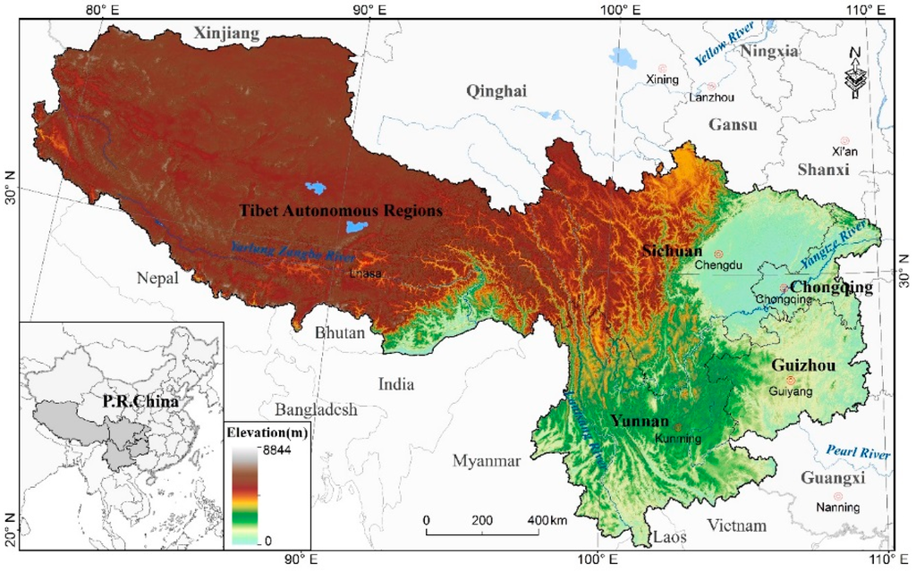
Figure 1.
The location of Southwestern China.
3. Methodology
3.1. Overall Description
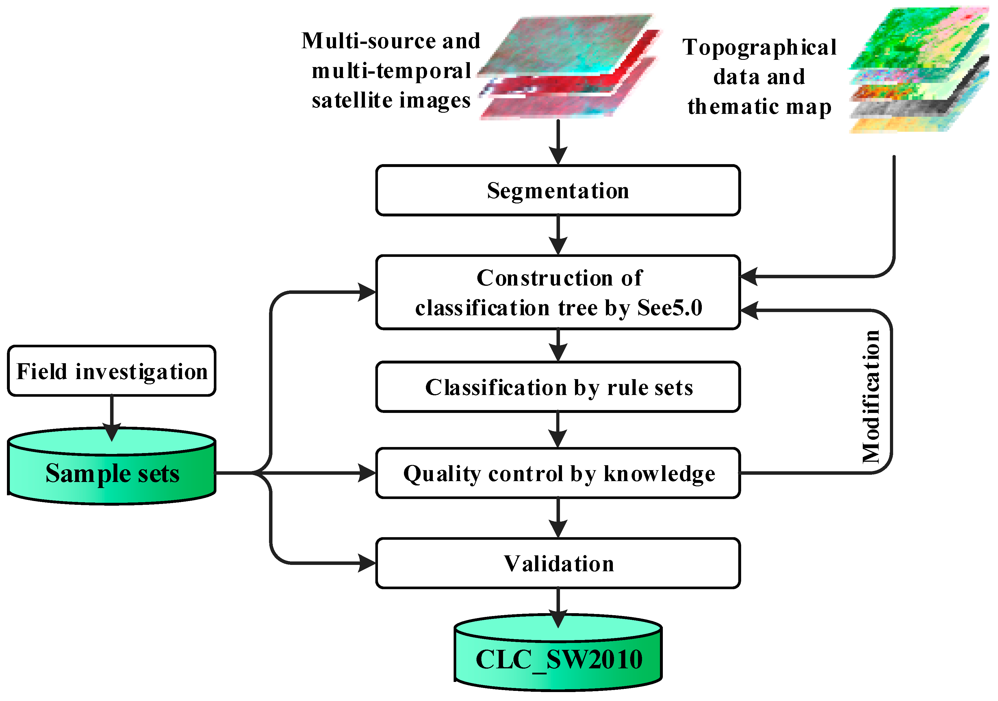
A new HC-MMK approach (Hierarchical Classification based on Multi-source and Multi-temporal data and geo-Knowledge) was proposed in this study to produce the 30 m-resolution CLC-SW2010 product, which is essentially an object-oriented classification method. The multi-source and multi-temporal satellite images and field data were firstly collected and preprocessed. After object-oriented multiresolution segmentation, a series of hierarchical classification trees for each mapping unit were built by decision tree algorithm and were then conducted to produce the preliminary classification results. Then, five-step knowledge-based interactive quality control was used to further improve the quality of classification results. The CLC-SW2010 product was independently validated by a third-party group. The construction of hierarchical classification trees and the five-step knowledge-based interactive quality control are the major components of this proposed approach. The flowchart of this proposed approach can be seen in Figure 2.

Figure 2.
The flowchart of the HC-MMK (Hierarchical Classification based on Multi-source and Multi-temporal data and geo-Knowledge) approach.
3.2. Land Cover Classification System
The classification system of China land cover for carbon budget [35] was adopted in this study, which includes two levels (Table 1). The first level has six land cover classes, including woodlands, grasslands, wetlands, croplands, artificial surface lands and bare lands. The basic 38 classes at the second level are formed by taking into full consideration the interpretation abilities of satellite imagery and the application demands of the Carbon Special Program and Ecological Decade Project. The land cover classes in this system are able to easily reorganize according to application requirements, and also are compatible with international land cover classification systems, such as FAO LCCS [35]. For more details on each land cover class, refer to the article by Zhang et al. [35].

Table 1.
Land cover classification system of the CLC-SW2010 product.
3.3. Remote Sensing Data Collection and Mapping Units
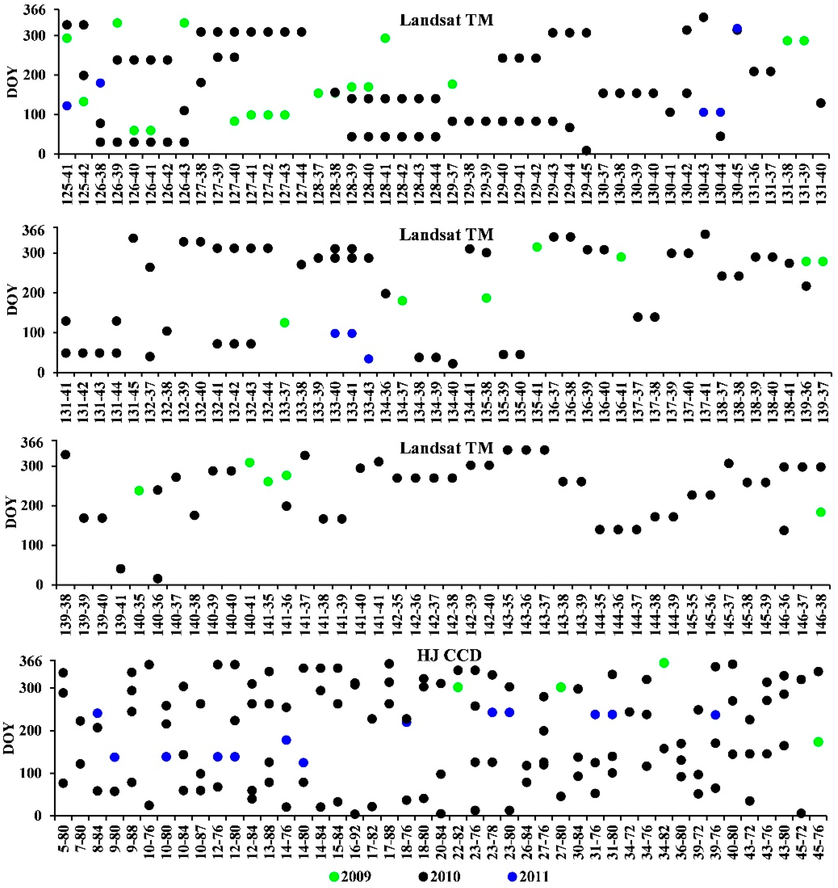
A total of 170 Landsat TM scenes and 202 HJ-CCD scenes were collected respectively from the USGS EarthExplorer and the China Center for Resources Satellite Data and Application. These images were acquired in 2009, 2010 and 2011 (Figure 3). For each mapping unit, at least two free-cloud satellite images (cloud coverage below 10%), one acquired in leaf-on conditions (May to October) and the other acquired in leaf-off conditions (November to following April), were selected to form the multi-temporal satellite images.

Figure 3.
The temporal distribution (DOY, day of year) of Landsat TM images and HJ-CCD images for each tile in Southwestern China. The X-axis was the scenes (path-row) of the Landsat TM images and the HJ-CCD images.
The acquired Landsat TM images have been calibrated radiometrically and geometrically. The atmospheric correction for the Landsat images were processed by the Landsat Ecosystem Disturbance Adaptive Processing System (LEDAPS, [36]). Although systematic geometric correction has been conducted, there are still some residual geometric errors existing in the acquired HJ-CCD images. The precise geometric correction for these HJ-CCD images was conducted by Auto-Registration and Orthorectification Algorithm [23], which was specially designed for satellite images over mountainous areas. After processing, the geometric errors between HJ-CCD images and Landsat TM images were less than one pixel [37].
The topographical data were incorporated in the classification, including elevation, aspect and slope. Despite some geo-location errors (approximately 1–3 pixels) existing in the 30-m ASTER GDEM in this region [38], it was still used in this study having less missing data, higher spatial resolution and better topographic representation than other elevation data (Such as SRTM) [39]. Using the ASTER GDEM data, the slope and aspect were calculated by the ERDAS software. The high spatial resolution Google Earth images and existing thematic maps, including the Vegetation Map of the People's Republic of China (1:1,000,000) and the Chinese Land Use Database at 1:100,000 scale, were also used for generating the CLC-SW2010 product. Although these thematic maps and high spatial resolution images were not directly used in the automatically classification due to the scale and quality, they could provide lots of useful reference information for sample selection and classification error identification.
To conveniently and efficiently organize a large number of satellite images and relevant auxiliary data, the study area needs to be partitioned into a series of mapping units according to the image scenes. Because distinct differences have existed between the HJ image scenes and the Landsat image scenes, neither Landsat image scenes nor HJ image scenes, but rather the intersection regions between HJ and Landsat image scenes were chosen to divide Southwestern China into 190 mapping units. All satellite images and ancillary data were clipped by these mapping units. Meanwhile, all processes including segmentation, automatic classification and quality control were conducted in these mapping units. Notably, a part of the overlapping regions needed to be retained to meet the requirements for mosaicking the final classification results for each neighboring mapping unit.
3.4. Field Data Collection
Three collection modes of field land cover samples have been designed at the initial phase of the Carbon Special Program and the Ecological Decade Project to collect as many field samples as possible. A total of 35,792 field samples have been collected in this area. For each field sample, the predominant land cover class, the geographical position and the field photos were recorded.
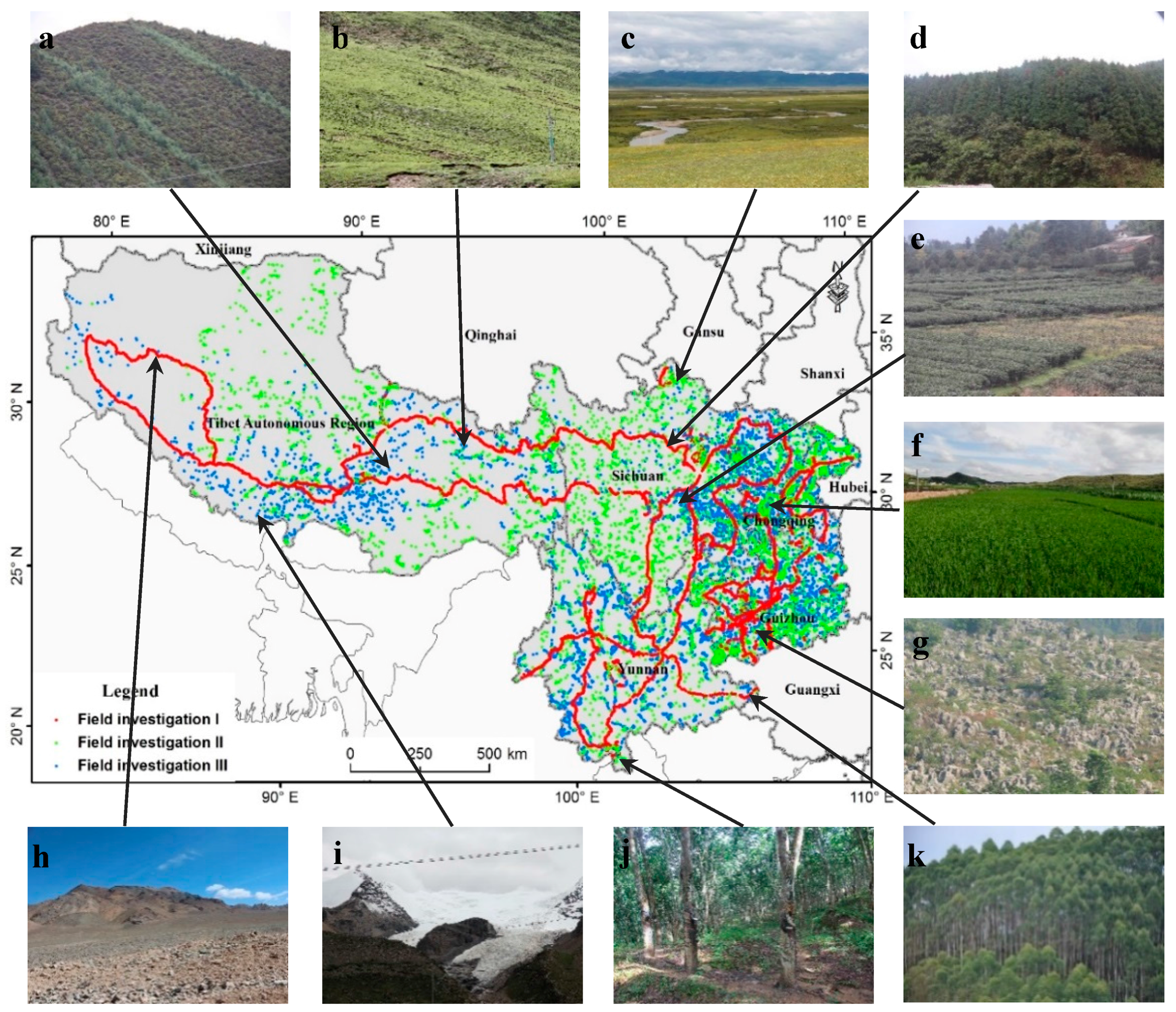
The first mode was designed to collect the field samples located around 2 km from the main road and the distance of two neighbor field samples was less than 3 km. Based on this mode, 16,721 field samples were collected in 2011 and 2012 by the mapping group. Meanwhile, the independent validation group collected 4546 field validation samples in 2011 by the same mode, which were only used to assess the accuracy of the CLC-SW2010 product. All field samples collected by the first mode are shown by solid red dots in Figure 4.

Figure 4.
The spatial distribution of field samples used for generating the CLC-SW2010 product. The pictures (a–k) represent respectively the deciduous broadleaf shrubs, meadows, herbaceous wetlands, evergreen needleleaf forests, tea garden (shrub plantations), paddy fields, karst vegetation (herbosa), bare soils, permanent snow and ices, rubber plantations (woody plantations) and eucalyptus plantations (woody plantations).
The second mode was used to collect the field samples in the predefined plots, including forest plots, grassland plots, shrub plots and cropland plots. More than 10 field samples were randomly distributed in each sample plot. These field investigation tasks were conducted by scientific survey teams from the Carbon Special Program, including forest survey teams, grassland survey teams, remote sensing survey teams, etc. A total of 6772 field samples (shown by solid green dots in Figure 4) were provided to the mapping group, 1378 of which were not provided until the accuracy assessment was completed.
The purposes of the third mode for collecting field samples were neither to train rule sets nor to evaluate the accuracy, but rather to discover the classification errors in the preliminary classification results. In this mode, about 20 field verification points were randomly chosen by the stratified sampling method for each county-level administrative division. Supported by local governments, a total of 7553 verification points (shown by solid blue dots in Figure 4) were collected by hundreds of staff from the local environmental authorities.
3.5. Object-Oriented Multi-Resolution Segmentation
Image segmentation is a crucial step in object-oriented classification, which groups homogenous neighboring pixels into meaningful objects. In this study, a wide-used multi-resolution segmentation algorithm [40,41] embedded in the platform Cognition 8.7 was adopted to segment satellite images. The scale, shape and compactness are three critical parameters. The optimal values of these parameters were determined by the trial-and-error method and visual assessment of the segmentation results. For the highly heterogeneous landscape, the scale parameter was set as 25, the shape parameter was set as 0.1 and compactness as 0.7. All of the Landsat images and the HJ images were incorporated in the segmentation process, except the topographical data and available thematic maps.
3.6. Hierarchical Classification Trees Construction by Decision Tree Algorithms
The hierarchical classification improved the quality of the land cover product in mountainous areas by increasing the classification times and decreasing the number of land cover classes within a single classification process. The whole classification process was divided into multiple stages according to the conceptual hierarchical structure in this study. For each classification stage, an optimal classification tree was constructed from the given training sample sets and classification feature sets by using the decision tree classifier (See5 software, https://www.rulequest.com/see5-info.html). Then, it was conducted to assign a unique land cover class for each object. Inevitably, this process was executed iteratively by adjusting the input training sample sets and feature sets until a satisfactory classification result was achieved in each classification stage. The hierarchical classification trees of each mapping unit were constructed independently. Training sample sets, classification feature sets and the conceptual hierarchical structure are the critical parts for classification tree construction.
3.6.1. Training Sample Sets
A total of 22,115 field samples collected by field investigations (detailed description shown in Section 3.4) were conducted to build the classification trees. For each mapping unit, because the assigned field samples are usually limited and unevenly distributed in space, many supplementary training samples were appended. These samples came from the visual interpretation of selected satellite images by the experienced mappers. Meanwhile, the existing field samples and high spatial resolution Google Earth images also provided references for the visual interpretation.
3.6.2. Multi-Type Classification Feature Sets
In this study, more than 40 features, including spectral features, topographic features, texture features and shape features, were conducted for constructing classification trees and automatically classifying for each mapping unit, which are shown in Table 2. Some satellite-derived indices were also involved in classification feature sets, including the Normalized Difference Vegetation Index (NDVI), the Modified Normalized Difference Water Index (MNDWI, [42]), and the Normalized Difference Built-Up Index (NDBI, [43]). All of selected features were calculated in the eCognition 8.7 platform. For spectral features, the mean value and the standard deviation of each band of multi-temporal satellite images were involved.
Table 2.
The multi-type features used in land cover classification. The b1, b2, b3, b4 and b5 denote respectively the blue, green, red, near infrared and mid-infrared band of satellite images. The GLCM is gray level co-occurrence matrix, which has a good ability to distinguish texture features of natural objects. The bv is the border length of image object, and the pv is the area of image object.
3.6.3. Conceptual Hierarchical Structure
Identifying the main land cover characteristics in each mapping unit and establishing a proper conceptual hierarchical structure are essential for the construction of hierarchical classification trees. Because the spectral signatures and the distinguishing capabilities of land cover class varied with the acquisition time of satellite images, the conceptual hierarchical structure needs to vary with mapping units. Figure 5 shows a representative conceptual hierarchical structure used for classification in a randomly selected mapping unit. It is noted that the structure in Figure 5 will not always be suitable for other mapping units.
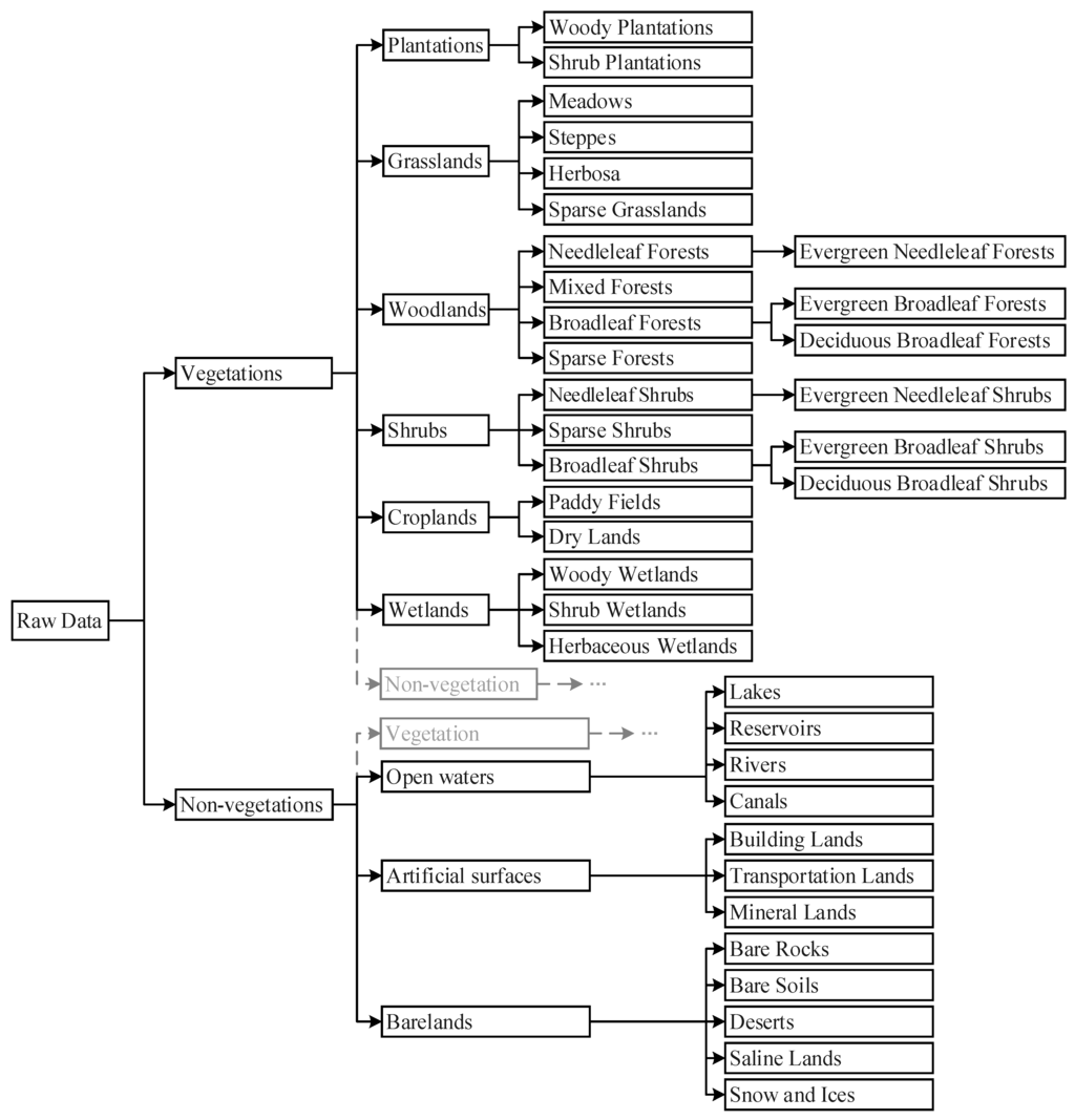
Figure 5.
A representative conceptual hierarchical structure of the land cover classes used for generating the CLC-SW2010 product.
For each hierarchical structure in Figure 5, the classification errors were hard to avoid in the classification results, which could be introduced into the following hierarchical levels. Therefore, these errors in the following hierarchical level needed to be revised. For example, some non-vegetation might be confused with vegetation, so the misclassified non-vegetation needed to be extracted in the vegetation division stage as well as following stages (Dish line in Figure 5). Owing to spatial limitations, Figure 5 only shows the handling of non-vegetation and vegetation, and the handling of other land cover classes is the same.
3.7. Five-Step Interactive Quality Control Based on Knowledge
3.7.1. Step One: Interactive Quality Control Based on Geographical Rules
The geographical rules, including the single-temporal rules and the multi-temporal geographical rules (list in Table 3), were used for inspecting the obvious errors in preliminary classification results. If the assigned land cover class of an object broke these rules, it would be revised by an automatic or manual method. The single-temporal rules were mainly concerned with the relationships between the land cover classes and the relevant geographical environment. For example, open waters usually reside in relatively flat or low relief areas. The multi-temporal rules paid more attention to those land cover classes which changed frequently with seasons. For instance, if an object was assigned as deciduous vegetation, but its spectral signatures did not demonstrate an obvious change within a year, this object was obviously misclassified and needed further revision.
Table 3.
The geographical rules used in the interactive quality control.
3.7.2. Step Two: Interactive Quality Control Based on Available Thematic Maps
The available thematic maps provided a lot of useful reference information, such as the predominated land cover class, the area ratio and spatial distribution of each land cover class, which were useful for discovering potential classification errors in the preliminary classification result. To effectively use this information, a series of comparisons between the CLC-SW2010 product and available thematic maps were conducted. Once any inconsistencies occurred and were caused by the classification errors, the mapper would further revise classification errors by an automatic or manual method according to the area of classification errors, until any significant differences did not appear in the comparison results.
The location map of the township government (hereinafter referred to as township map) was used to discover the omitted residential land in the preliminary classification result in this study. It is difficult to extract automatically the residential land only relying on the spectral features, because the residential land in mountainous areas are usually composed by dispersed rural houses. The township governments are an important indicator for the residential land because they are usually situated in the concentrated regions of residential land. In this study, under the guidance of the township map and leaf-on satellite images, the omission residential lands were added artificially.
3.7.3. Step Three: Spatial Consistency Verification
The spatial discontinuity phenomena of land cover often occurred at the junction regions of the neighbor mapping units in classification results, which were mainly caused by the following differences: the acquisition time of selected satellite images in neighboring mapping units and the cognitive level of mappers. Therefore, the spatial consistency verification is indispensable to assuring the quality of the CLC-SW2010 product. To avoid any inspection omission, the whole of Southwestern China was divided into 24,130 grids with a side length of 10 km. The experienced mapper carefully checked and revised the spatial discontinuous phenomena grid by grid.
3.7.4. Step Four: Interactive Quality Control with Field Verification Points
To discover any further residual classification errors in the CLC-SW2010 product, a new round of field investigation was enforced to collect independent verification points (Section 3.4). The experienced mappers were carefully compared with the classification results of each verification point and its surrounding regions with the field records, photos and satellite images. Once the classification errors were determined, further revisions were needed.
3.7.5. Step Five: Interactive Quality Control with Statistics Reports
Some recognized statistical information, such as forest coverage, grassland area and cropland area, was recorded in government statistics reports and relevant documents, which were helpful for verification of the quality of the CLC-SW2010 product. Unfortunately, the differences of the definition for the same land cover classes have existed between the statistics report and the CLC-SW2010 product. Only when the differences of the area of a certain land cover class exceeded a predefined threshold value (10% of its area), should further revision be considered.
4. Results
4.1. Hierarchical Decision Tree
For each mapping unit, a series of classification trees generated by the decision tree classifier (See Section 5) were conducted to produce the CLC-SW2010 product in this study. Owing to spatial limitations, this paper only shows three typical decision trees, which were conducted for distinguishing between vegetation and non-vegetation, vegetation divisions and forest divisions, respectively, in the junction zone (path/row: 138/38, WRS2) of the Sichuan province and Tibet autonomous region.
4.1.1. The Decision Tree for Distinguishing Vegetation and Non-Vegetation
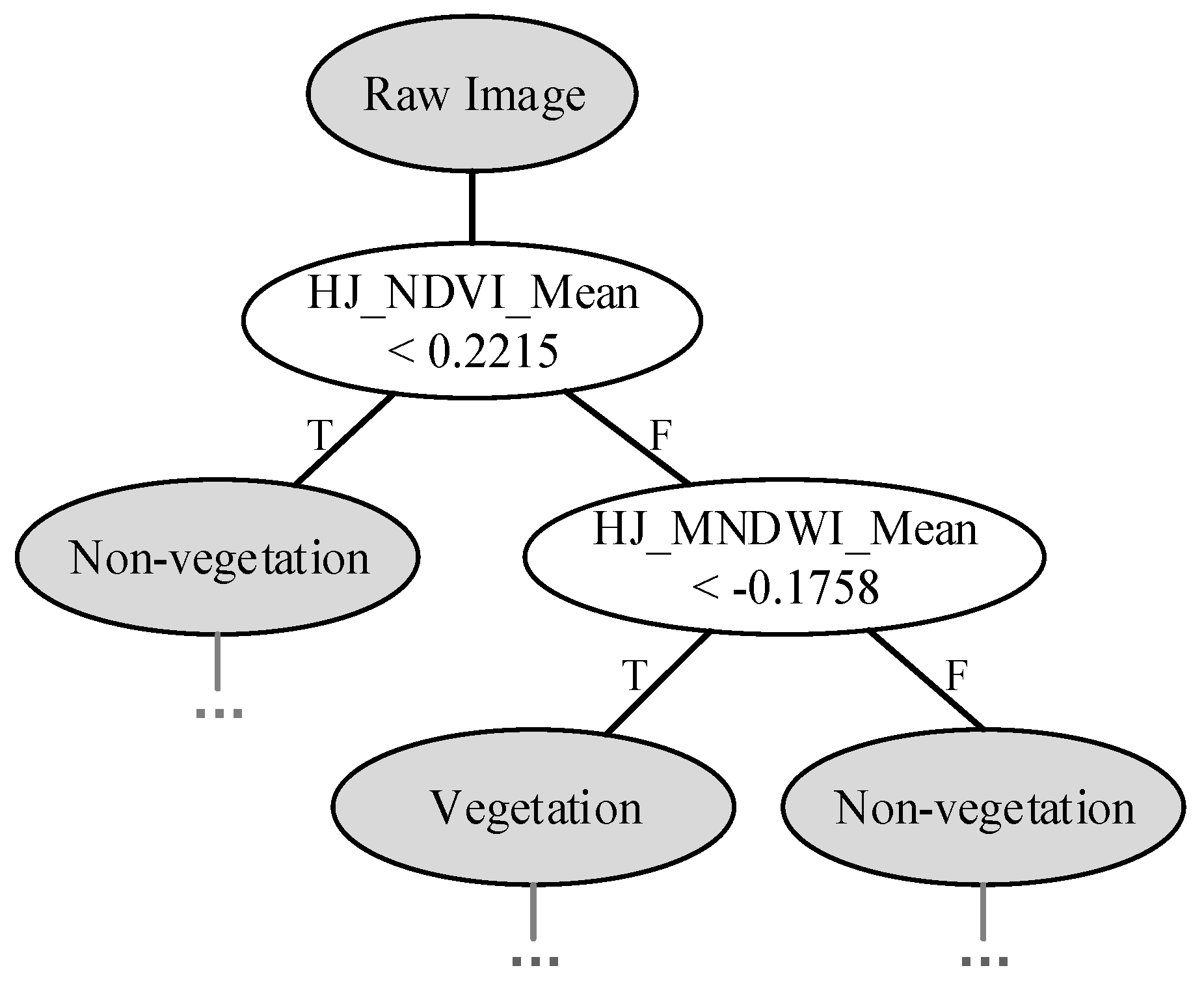
Figure 6 shows a typical decision tree for distinguishing vegetation and non-vegetation. Generally, the differences of NDVI between vegetation and non-vegetation in the leaf-on season are obvious. Therefore, the mean value of NDVI derived from the HJ image in leaf-on season was used to distinguish between non-vegetation and vegetation. Then the MNDWI derived from the same image was used to identify open waters misclassified as vegetation, because it is sensitive to open waters.

Figure 6.
The decision tree for distinguishing vegetation and non-vegetation. The HJ-CCD image acquired on 24 July 2010. The ellipsis represents the land cover class needed for further division.
4.1.2. The Decision Tree for Vegetation Division
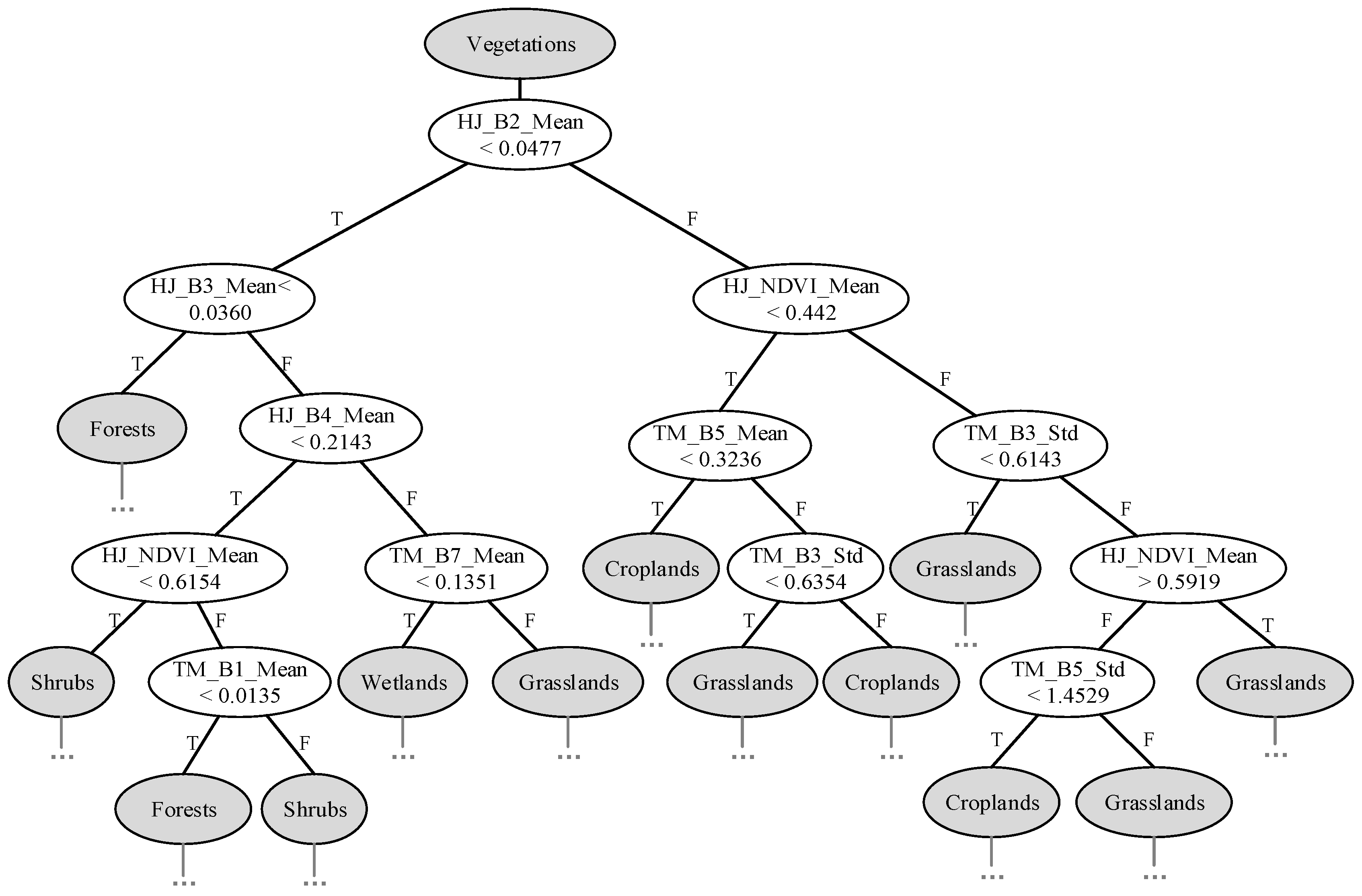
The vegetation extracted by above decision tree were further divided into forests, shrubs, grasslands, wetlands (covered with herbaceous and woody vegetation) and croplands by the decision tree shown in Figure 7. Obvious differences between the herbaceous vegetation (including withered grasslands and harvest croplands) and the woody vegetation (including shrubs and forests) existing in spectral reflectance of green band of leaf-on satellite images. Therefore, the feature of HJ_B2_Mean was used to distinguish them. In leaf-on season, the NDVI values (HJ_NDVI_Mean) between croplands and grasslands have differences, which were chosen to separate grasslands and croplands. The standard deviation of red and mid-infrared bands (TM_B3_Std and TM_B5_Std) was applied to reduce the commissions between grasslands and croplands because cropland objects usually have a higher degree of dispersion of spectral reflectance than grassland objects. Using the absorption feature of forest canopy in the red band (HJ_B3_Mean), the forests were extracted from the woody vegetation. The wetlands have relatively low reflectance in the near-infrared band (HJ_B4_Mean) due to the absorption feature of water, which was adopted to distinguish between wetlands and shrubs. The forests confused with the shrubs were extracted again by the spectral reflectance of blue band in leaf-off satellite images (TM_B1_Mean), and the grasslands confused with the croplands were extracted again by the spectral reflectance of mid-infrared band in leaf-off satellite images (TM_B7_Mean). Above all, each satellite image played a unique role and the multi-temporal satellite images contributed to effectively discriminating between each vegetation type.

Figure 7.
The decision tree for vegetation division. The Landsat TM image acquired on 28 September 2010. The Bx denotes x-th band of satellite image, the Std denotes the standard deviation.
4.1.3. The Decision Tree for Forests Division
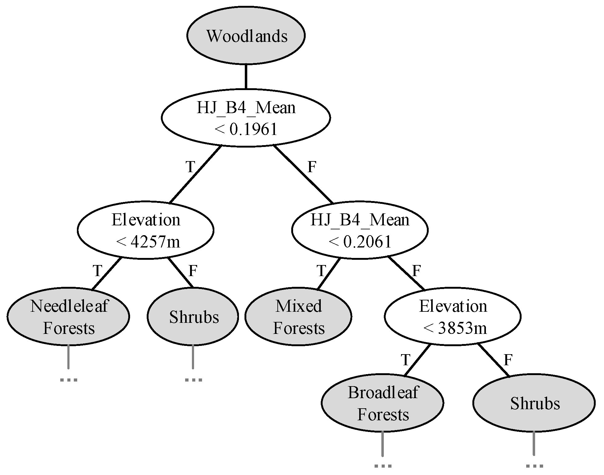
Usually, the distinct differences existed in the near-infrared band of leaf-on satellite images among broadleaf forests, the needleleaf forests and the mixed forests, which were used to separate forests into broadleaf forests, needleleaf forests and mixed forests (Figure 8). The spatial distributions of each forest display distinct vertical stratification in mountainous areas, which was useful for discovering and revising classification errors of vegetation types. For example, the shrubs misclassified as needleleaf forests and broadleaf forests were extracted by the Elevation in Figure 8.

Figure 8.
The decision tree for woodlands divisions.
4.2. Effectiveness of Interactive Quality Control
The five steps of knowledge-based interactive quality control were not conducted simultaneously. The steps based on geographical rules and the thematic maps were applied firstly in the automatic classification stage, and then the spatial consistency checking was conducted after forming a whole land cover map. The steps based on the verification points and statistics information were used in the last stage. Although all five steps were conducted to revise the classification errors contained in the CLC-SW2010 product, this section only shows two representative examples due to space limitations.
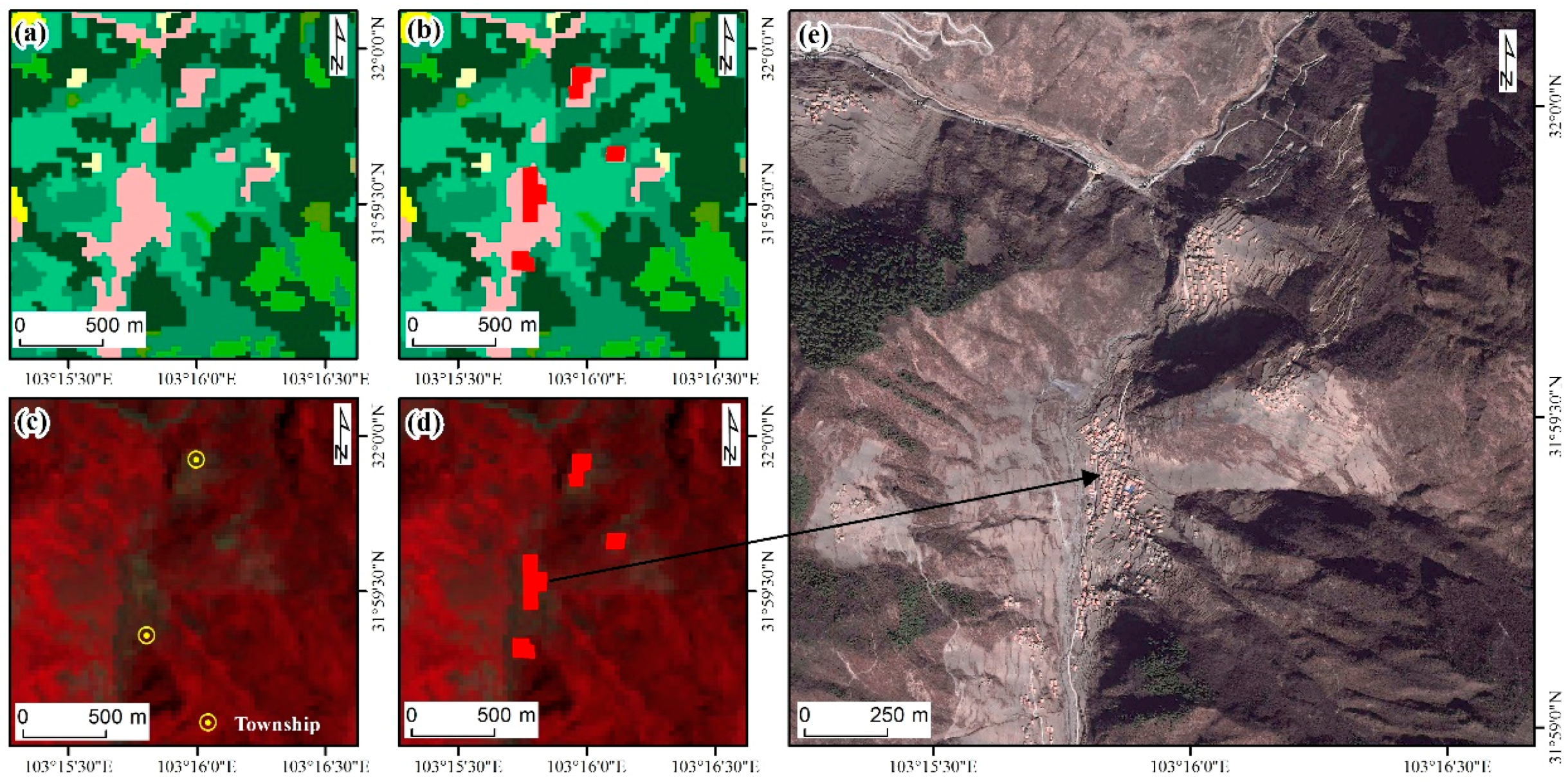
Figure 9 shows a typical example for revising residential land at high altitude by using a township map. The residential land in mountainous areas was often omitted by automatic classification approaches, but this omitted residential land was artificially added with the help of the township map and the high-resolution Google Earth images.

Figure 9.
Interactive quality control based on the existing thematic map (township map). (a) and (b) are the results of unrevised and revised residential lands, respectively; (c) is the Landsat TM images and the locations of township; (d) is the additional residential lands with the help of the township map and high-resolution satellite images; (e) is the high-resolution Google Earth images.
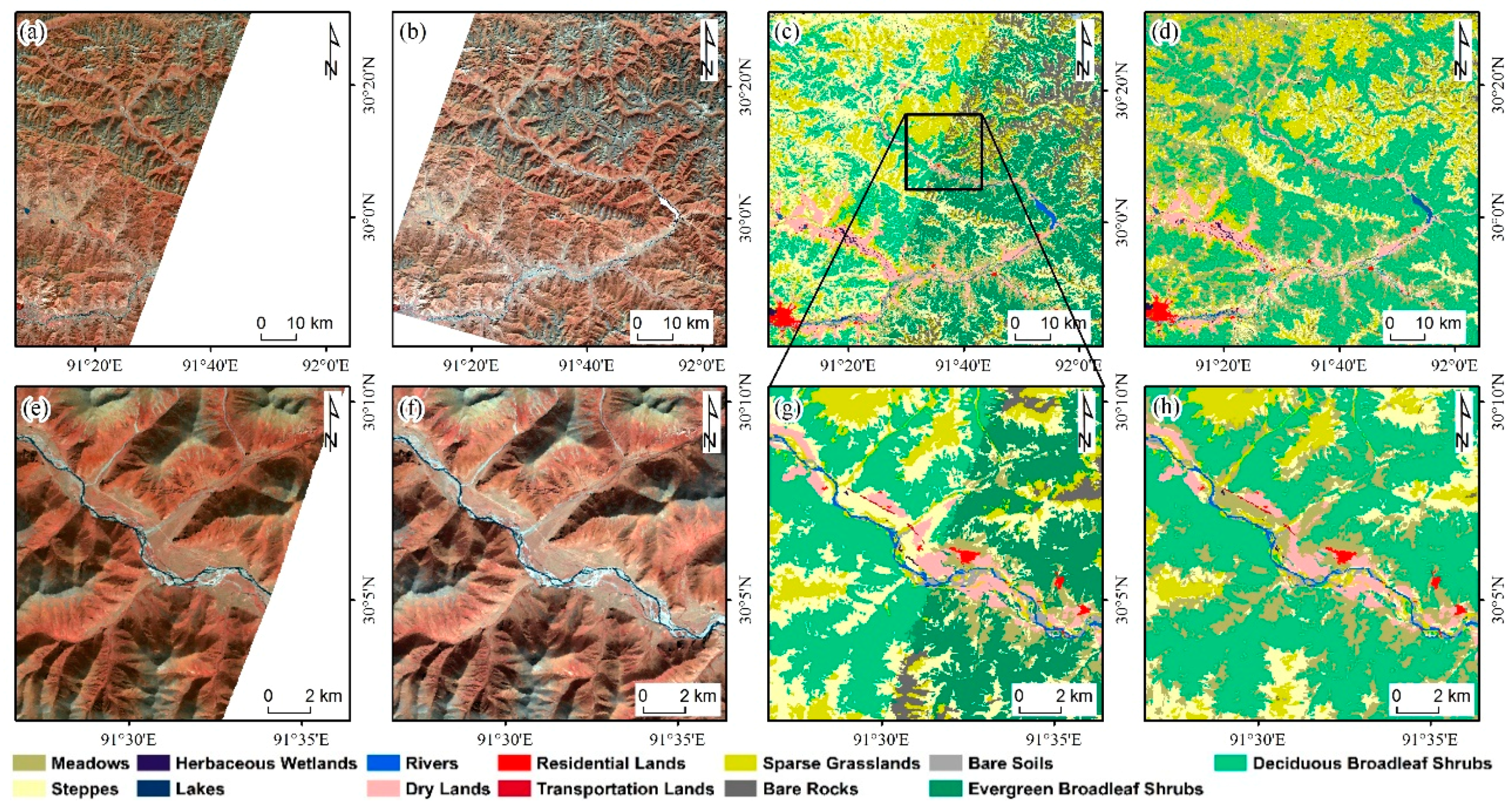
A typical spatial discontinuous phenomenon is shown in Figure 10c,g, which mainly comes from confusing the evergreen shrubs with the deciduous shrubs. In this case, the classification trees used for distinguishing the evergreen shrubs and the deciduous shrubs needed to be reconstructed by adjusting training sample sets and feature sets for each mapping unit until a satisfactory result was obtained. After revision, the spatial discontinuous phenomenon was removed in the post-checking classification results (Figure 10d,h).

Figure 10.
The results of the spatial consistency checking. (a) is the Landsat TM images (path/row: 138/39, acquired on 17 October 2009) used for classification of left mapping unit; (b) is the Landsat TM images (path/row: 137/39, acquired on 26 October 2009) used for classification of right mapping unit; (c) is the pre-checking classification result; (d) is the post-checking classification result; (e), (f), (g) and (h) are the enlarged images at black box in the (a), (b), (c) and (d), respectively.
4.3. The CLC-SW2010 Product and Product Accuracy
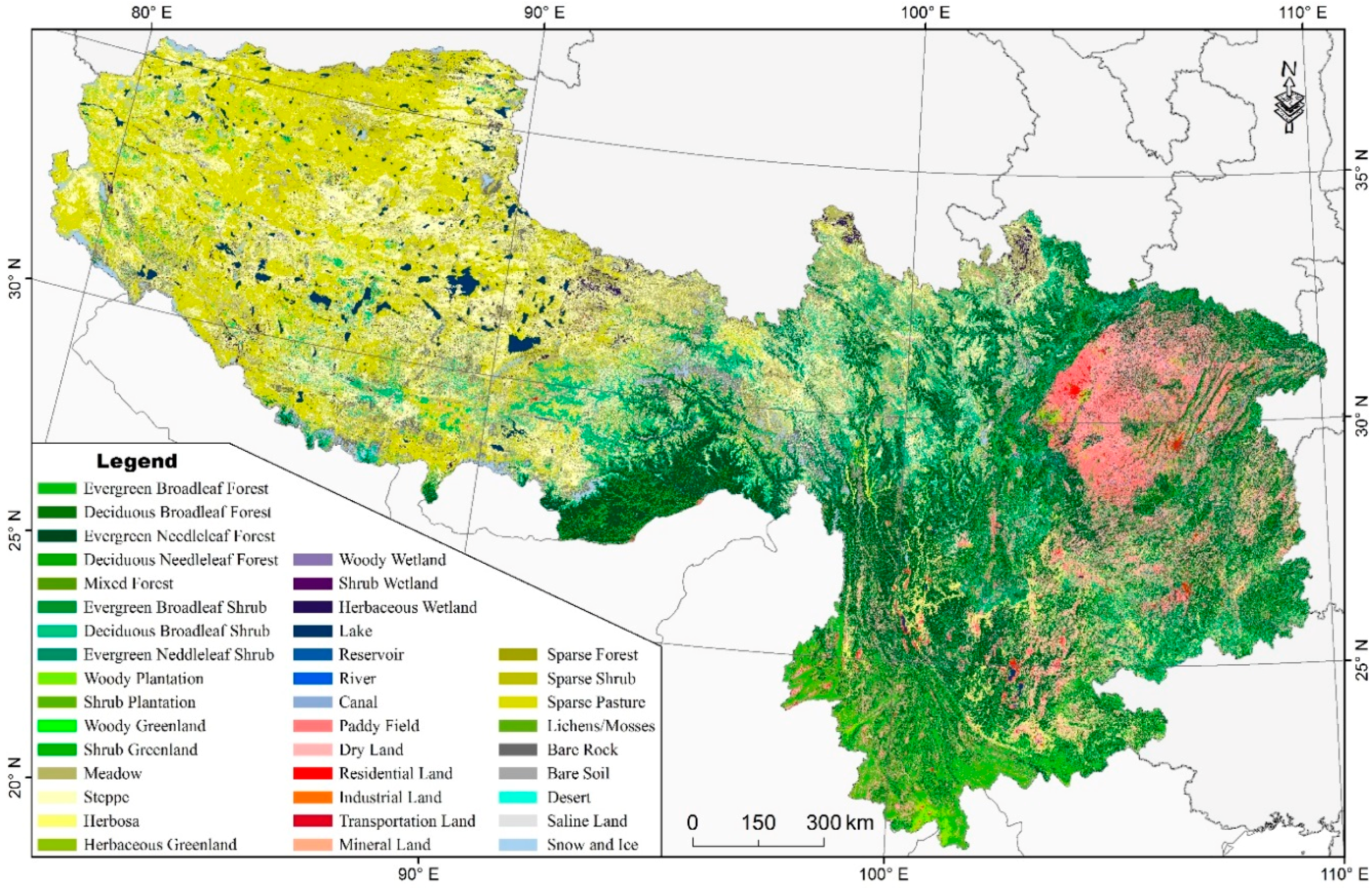
Taking the multi-temporal native HJ-CCD images and Landsat TM images as main input data, the 30 m-resolution CLC-SW2010 product (Figure 11) was produced by the proposed HC_MMK approach over the last three years.

Figure 11.
The CLC-SW2010 product.
In the CLC-SW2010 product, the grasslands and woodlands are the predominant land cover classes, accounting for 45.01% and 34.92% of the land area of Southwestern China, respectively. The areas of croplands and bare lands are less than that of grasslands and woodland, accounting for 10.45% and 6.10%, respectively. Artificial surfaces and wetlands are rarely found in Southwestern China, only accounting for 0.55% and 2.97%, respectively. The grasslands (including sparse grasslands) are mainly distributed on the Tibet plateau (81.06%), Western Sichuan plateau (11.21%) and the Karst region (7.73%). The woodlands are mainly found in Hengduan Mountain, Daba Mountain, Southeastern Tibet and Yunnan province. The cropland is mainly located in Sichuan Basin, Anning River valley and the “bazi” regions of Yunnan-Guizhou Plateau.
A total of 5924 validation points, which have been collected independently by a third-party group, were conducted to assess the accuracy of the CLC-SW2010 product. After independent validation, the accuracy of the primary categories and secondary categories of the CLC-SW2010 product reached 95.09% and 87.14%, respectively, and the kappa coefficients were 0.9345 and 0.8573 respectively. The detailed precision information of the CLC-SW2010 product is shown in Table 4 and Table 5.
Table 4.
The confusion matrix of primary categories in the CLC-SW2010 product. The codes of each primary category are the same as the ones listed in Table 1.
Table 5.
The confusion matrix of secondary categories in the CLC-SW2010 product.
The wetlands and bare lands have a higher accuracy (>98%) than other land cover classes, and the accuracy of the grasslands is in the end in CLC-SW2010 (Table 4). Confusing with croplands and shrubs is the main reason for grassland inaccuracy. Because the grasslands were usually accompanied by shrubs, especially in the Karst mountainous area, it is difficult to accurately distinguish the grasslands and the shrubs [46]. They have a similar spectral signature between the grassland and the returned farmlands with 15–25 degree slopes. Therefore, these returned farmlands were frequently classified as croplands rather than grasslands in the CLC-SW2010 product.
The evergreen needleleaf forests, herbaceous wetlands, rivers, lakes, reservoirs, paddy fields, residential lands and permanent snow and ice have a higher user’s accuracy and producer’s accuracy than other secondary categories (Table 5). The multi-source and multi-temporal satellite images, geo-knowledge, objected-oriented method and hierarchical classification played its roles in the accuracy of the CLC-SW2010 product. For instance, the spectral and shape signatures of the lakes were highly similar to the reservoirs. However, obvious differences existed in the spatial distribution between the lakes and the reservoirs in Southwestern China, the former mainly distributed in the plateau, and the latter mainly located in the agricultural region, which were useful for exactly distinguishing the lakes and the reservoirs.
5. Discussions
5.1. Comparison with Existing 30 m-Resolution Land Cover Products
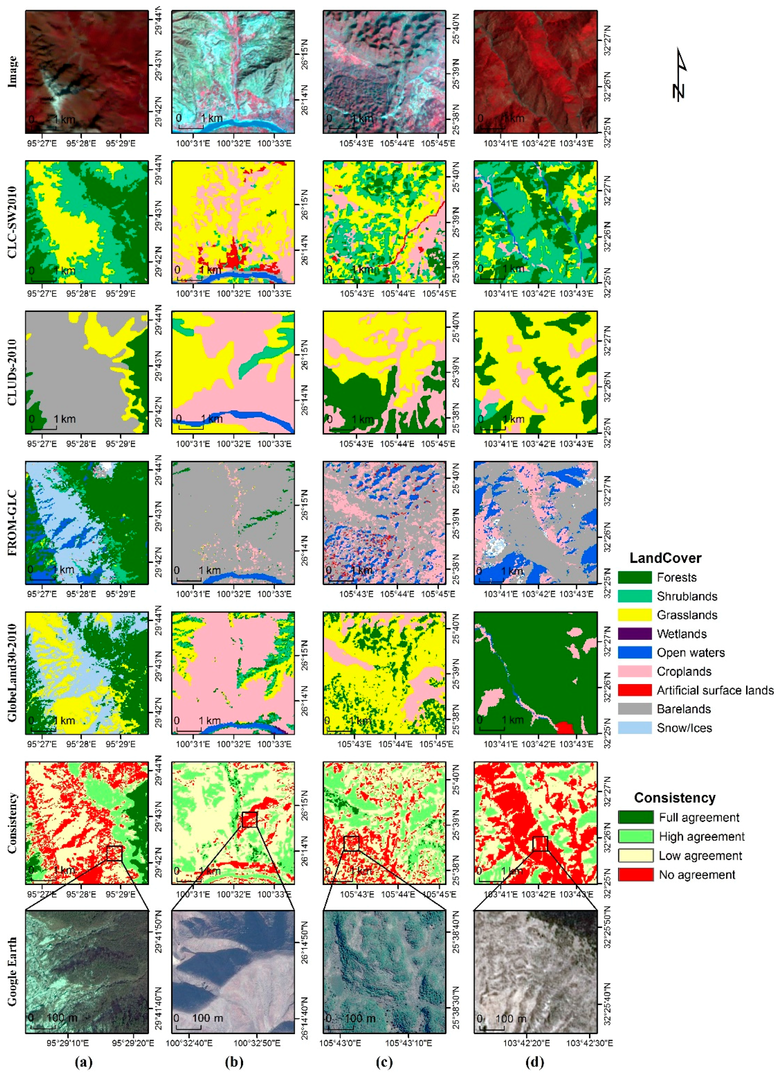
The CLC-SW2010 product were compared with other existing 30 m-resolution land cover products in 2010 over Southwestern China, including CLUDs (the third row of Figure 12), FROM-GLC (the fourth row of Figure 12) and GlobeLand30 (the fifth row of Figure 12). It was found that the quality of CLC-SW2010 was superior to these products according to the respective preliminary validation results, the accuracy of FROM-GLC and GlobeLand30 reached 71.54% [5] and 80.33% ± 0.2% [11], respectively. The lack of leveraging variability in phenological patterns is an important factor for the quality of GlobeLand30 and FROM-GLC [18]; however, it has been avoided in CLC-SW2010 by introducing multi-temporal satellite images and a variety of geo-knowledge. Although the total area of each land cover class is closer to reality, the boundary of land cover is vague and inaccurate in CLUDs (the third row of Figure 12).

Figure 12.
The comparison of classification results among four land cover products in four typical regions. The regions of (a–d) are located in Southeast Tibet, the middle part of Yunnan province, the Karst region of Guizhou province and the upper reaches of Minjiang River, respectively. For the consistency of pixels, the full agreement denotes all four products have a same land cover class, high agreement denotes there are two land cover classes among four products, low agreement denotes there are three land cover classes among four products and no agreement denotes there are a unique class in each product.
Four typical mountainous regions that are hard to map (a: Plateau regions host mostly grasslands; b: low mountains mainly consist of croplands; c: Karst regions with complex land cover and d: steep mountainous areas mostly covered with forests) were taken as examples (Figure 12) to present the comparison results of four land cover products in detail. The CLC-SW2010 product showed more distinctly the vertical stratification of vegetation (Figure 12a) and the fragmentized landscape (Figure 12b,c) in mountainous areas than the other three products, and the proposed HC-MMK approach especially designed for land cover mapping in mountainous areas was the main contributor. There was also many classification errors identified between mountain shadow and water in FROM-GLC (the fourth row of Figure 12), which were eliminated by some simple geographical rules in CLC-SW2010.
5.2. The Contribution of Each Component in the HC-MMK Approach
5.2.1. The Multi-Source and Multi-Temporal Data
In this paper, the native HJ-CCD images and Landsat TM images have been combined to provide more high-quality satellite images (Figure 3) for generating the CLC-SW2010 product. This combination can maximize the advantages of the native HJ-CCD images (wide-covered and short repeat cycle) and the Landsat TM images (plentiful spectral information and excellent quality). The multi-temporal satellite images were useful for distinguishing the evergreen vegetation and the deciduous vegetation, because they have differences in changes of spectral signature between leaf-on season and leaf-off season [19]. Meanwhile, the temporal signatures were used for identifying the dry lands, paddy fields and other land cover classes, and their spectral signatures frequently varied with season in this study.
5.2.2. Knowledge
The importance of knowledge for producing land cover products has been well acknowledged [11,16,47,48]. Subject to the availability, scale and quality of knowledge, at present, limited knowledge has been drawn upon to enhance the accuracy of land cover products, such as terrain knowledge [16,49], spatial distribution knowledge [11], and temporal signature [18,50,51]. In this paper, a variety of available knowledge, including geographical rules, existing thematic maps, field samples and statistical information, were applied together in the HC-MMK approach. Each type of knowledge played a unique role and all knowledge together contributed to quality improvement of the CLC-SW2010 product (Figure 9 and Figure 10). The attempt to draw upon of variety of knowledge in this study offered a recommendable method for other land cover mapping projects.
5.2.3. Hierarchical Classification
Hierarchical classification is an effective land cover mapping method for those areas with complex and heterogeneous landscapes by increasing classification time and decreasing the number of land cover classes in a single classification process [52,53,54]. The conceptual hierarchical structure is the core of this approach. A unique conceptual hierarchical structure was built in most research [53,54], which cannot meet the demands for land cover mapping over large regions with complex terrain, such as Southwestern China, because there are 38 land cover classes, 190 mapping units and various land cover classes. To solve this problem, a series of conceptual hierarchical structures aimed for each unique mapping unit were built in this study, which obviously improved the accuracy of the CLC-SW2010 product. This strategy also provided a useful reference for future research on land cover mapping over large areas.
5.2.4. Quality Control
Quality control is a critical step for producing a widely-used land cover product [11,55,56]. The procedures need to be applied to the whole classification process, including satellite image collection and preprocessing, field data collection, automatic classification and accuracy assessment. Only if each sub-step obtained a high-precision result could a high accuracy land cover product be achieved. This paper proposed a practical, interactive quality control method based on prior knowledge, which obviously eliminated many classification errors and spatial discontinuity phenomena (Figure 9 and Figure 10) and improved the quality of the CLC-SW2010 product. In addition, many strict criteria were also developed in the other stages; for instance, the accuracy of image-to-image co-registration was less than 2 pixels in mountainous areas for data preprocessing, and the total cloud cover was less than 10% for each selected satellite image.
5.3. The Merits and Limitations of the Current Work
The land cover classification system used in the CLC-SW2010 was more suitable for various ecological applications than other classification systems, because it gave adequate consideration to life form, vegetation height, leaf type, vegetation phenology, vegetation cover, and so on [35]. In addition, this classification system was easy to interoperate with multiple land cover classification systems, such as FAO LCCS, which will help to widen the application scope of the CLC-SW2010 product. A full set of automatic mapping processes, including satellite image preprocessing, classification and quality control, were proposed in this study. They were conducted to generate the CLC-SW2010 product, which obviously shortened the mapping cycle. The main users, including the local environmental authorities and the research teams of the Carbon Special Program, have been involved in the process of generating the CLC-SW2010 product. They not only provided the field land cover samples, but also discovered potential classification errors existing in the CLC-SW2010 according to their experiences.
Using the proposed HC-MMK approach, the overall accuracy of the CLC-SW2010 reached 87.14%. However, there are still some limitations in the current mapping work. Due to the lack of floodplain wetlands in land cover classification systems, the floodplain wetlands were classified as bare soils in the CLC-SW2010 product. They will limit its applications because distinct differences of ecological structure and functions existed between the floodplain wetlands and the bare soils. Meanwhile, some land cover classes have a lower producer’s accuracy and user’s accuracy in the CLC-SW2010 product, especially for mixed forests, steppes and meadows. The vague and non-quantitative definition and various spectral signatures are the main causes for the low accuracy of the mixed forests. The spectral signatures of the steppes and the meadows are easy to vary with the species, coverage, biomass and moisture content, which impacted distinguishing between steppes and meadows in the CLC-SW2010 product. Therefore, it is worth exploring how to further improve the accuracy of the mixed forests, steppes and meadows and optimize the land cover classification system according to application demands in the future.
6. Conclusions
This paper mainly introduced the proposed HC-MMK approach and the 30 m-resolution CLC-SW2010 product. The multi-temporal native HJ-CCD images, Landsat TM images and topographical data were taken as the main input data in this study. Hierarchical classification tree construction and a five-step knowledge-based interactive quality control were the key components of this proposed approach. Based on independent accuracy assessment by a third-party group, the overall accuracy of primary and secondary categories of the CLC-SW2010 product reached 95.09% and 87.14%, respectively, and the Kappa coefficients were 0.9345 and 0.8573, respectively.
To address critical issues for land cover mapping in mountainous areas, four key steps were taken in this study. Firstly, a combination of the native HJ-CCD images and Landsat TM images were taken as input data to construct the multi-temporal satellite images. Secondly, the satellite images with complex terrain were segmented with as much detail as possible in the image segmentation stage. Thirdly, for each mapping unit, a series of unique hierarchical classification trees were built to make the land cover classification as accurate as possible. Finally, a variety of prior geo-knowledge, including geographical rules, existing available thematic maps, verification samples and statistical information, was extensively used in the classification and quality control stage to improve the accuracy of the product.
The proposed HC-MMK approach can be used not only in mountainous areas, but also in plains, hills and other regions, because land cover mapping in mountainous areas is more complex than other regions. Overall, this study proposed an operable land cover mapping method and produced a 30 m-resolution CLC-SW2010 product. Most importantly, it provided an important reference point for other land cover mapping studies conducted over large areas or even the entire globe in the future.
Acknowledgments
This research was funded jointly by the Strategic Leader Science and Technology project (XDA05050105), the “Ecology decade” specific project of MEP&CAS (STSN-01-04), the International Cooperation Key Project of CAS (GJHZ201320) and the National Natural Science Foundation of China (41271433, 41571373). We are especially grateful to Bingfang Wu, Yuan Zeng and Lei Zhang for their support and advice. We are also thankful to all the contractors, image providers and the anonymous reviewers for their valuable comments and suggestions.
Author Contributions
All authors have made major and unique contributions. Ainong Li designed the framework of this research. Guangbin Lei drafted the preliminary version and Ainong Li finished the final version of the manuscript. Ainong Li, Guangbin Lei, Huaan Jin, Jinhu Bian, Xi Nan, Wei Zhao, Qiannan Liu, Guangbin Yang and Huan Yu took part in the field data collection. Jinhu Bian is in charge of satellite data collection and pre-processing. Guangbin Lei, Jinhu Bian, Zhengjian Zhang and Ainong Li completed the land cover mapping in Sichuan Province. Guangbin Lei, Huaan Jin, Jiyan Wang, Wei Zhao, Wenlan Feng, and Ainong Li completed the land cover mapping in Tibet autonomous region. Guangbin Yang, Guangbin Lei, Xiaomin Cao, Jianbo Tan and Ainong Li completed the land cover mapping in Guizhou province and Chongqing Municipality. Huan Yu, Xi Nan, Guangbin Lei and Ainong Li completed the land cover mapping in Yunnan provinces.
Conflicts of Interest
The authors declare no conflict of interest.
References
- Yang, J.; Gong, P.; Fu, R.; Zhang, M.H.; Chen, J.M.; Liang, S.L.; Xu, B.; Shi, J.C.; Dickinson, R. The role of satellite remote sensing in climate change studies. Nat. Clim. Chang. 2013, 3, 875–883. [Google Scholar] [CrossRef]
- Shupeng, C.; van Genderen, J. Digital Earth in support of global change research. Int. J. Digit. Earth 2008, 1, 43–65. [Google Scholar] [CrossRef]
- Gross, J.E.; Goetz, S.J.; Cihlar, J. Application of remote sensing to parks and protected area monitoring: Introduction to the special issue. Remote Sens. Environ. 2009, 113, 1343–1345. [Google Scholar] [CrossRef]
- Wiens, J.; Sutter, R.; Anderson, M.; Blanchard, J.; Barnett, A.; Aguilar-Amuchastegui, N.; Avery, C.; Laine, S. Selecting and conserving lands for biodiversity: The role of remote sensing. Remote Sens. Environ. 2009, 113, 1370–1381. [Google Scholar] [CrossRef]
- Gong, P.; Wang, J.; Yu, L.; Zhao, Y.C.; Zhao, Y.Y.; Liang, L.; Niu, Z.G.; Huang, X.M.; Fu, H.H.; Liu, S.; et al. Finer resolution observation and monitoring of global land cover: First mapping results with Landsat TM and ETM+ data. Int. J. Remote Sens. 2013, 34, 2607–2654. [Google Scholar] [CrossRef]
- Hansen, M.C.; Potapov, P.V.; Moore, R.; Hancher, M.; Turubanova, S.A.; Tyukavina, A.; Thau, D.; Stehman, S.V.; Goetz, S.J.; Loveland, T.R.; et al. High-resolution global maps of 21st-century forest cover change. Science 2013, 342, 850–853. [Google Scholar] [CrossRef] [PubMed]
- Loveland, T.R.; Reed, B.C.; Brown, J.F.; Ohlen, D.O.; Zhu, Z.; Yang, L.; Merchant, J.W. Development of a global land cover characteristics database and IGBP DISCover from 1 km AVHRR data. Int. J. Remote Sens. 2000, 21, 1303–1330. [Google Scholar] [CrossRef]
- Friedl, M.A.; Sulla-Menashe, D.; Tan, B.; Schneider, A.; Ramankutty, N.; Sibley, A.; Huang, X.M. MODIS collection 5 global land cover: Algorithm refinements and characterization of new datasets. Remote Sens. Environ. 2010, 114, 168–182. [Google Scholar] [CrossRef]
- Arino, O.; Bicheron, P.; Achard, F.; Latham, J.; Witt, R.; Weber, J.L. GlobCover the Most Detailed Portrait of Earth. Available online: https://earth.esa.int/web/guest/-/globcover-the-most-detailed-portrait-of-earth-5910 (accessed on 30 March 2016).
- Yu, L.; Wang, J.; Li, X.; Li, C.; Zhao, Y.; Gong, P. A multi-resolution global land cover dataset through multisource data aggregation. Sci. China-Earth Sci. 2014, 57, 2317–2329. [Google Scholar] [CrossRef]
- Chen, J.; Chen, J.; Liao, A.P.; Cao, X.; Chen, L.J.; Chen, X.H.; He, C.Y.; Han, G.; Peng, S.; Lu, M.; et al. Global land cover mapping at 30 m resolution: A POK-based operational approach. ISPRS J. Photogramm. Remote Sens. 2015, 103, 7–27. [Google Scholar] [CrossRef]
- Liu, J.Y. Study on national resources and environment survey and dynamic monitoring using remote sensing. J. Remote Sens. 1997, 1, 225–230. [Google Scholar]
- Liu, J.Y.; Kuang, W.H.; Zhang, Z.X.; Xu, X.L.; Qin, Y.W.; Ning, J.; Zhou, W.C.; Zhang, S.W.; Li, R.D.; Yan, C.Z.; et al. Spatiotemporal characteristics, patterns, and causes of land-use changes in China since the late 1980s. J. Geogr. Sci. 2014, 24, 195–210. [Google Scholar] [CrossRef]
- Giri, C.; Pengra, B.; Long, J.; Loveland, T.R. Next generation of global land cover characterization, mapping, and monitoring. Int. J. Appl. Earth Obs. Geoinf. 2013, 25, 30–37. [Google Scholar] [CrossRef]
- Kuenzer, C.; Leinenkugel, P.; Vollmuth, M.; Dech, S. Comparing global land-cover products-implications for geoscience applications: An investigation for the trans-boundary Mekong Basin. Int. J. Remote Sens. 2014, 35, 2752–2779. [Google Scholar] [CrossRef]
- Li, A.N.; Jiang, J.G.; Bian, J.H.; Deng, W. Combining the matter element model with the associated function of probability transformation for multi-source remote sensing data classification in mountainous regions. ISPRS J. Photogramm. Remote Sens. 2012, 67, 80–92. [Google Scholar] [CrossRef]
- Jia, K.; Liang, S.L.; Zhang, N.; Wei, X.Q.; Gu, X.F.; Zhao, X.; Yao, Y.J.; Xie, X.H. Land cover classification of finer resolution remote sensing data integrating temporal features from time series coarser resolution data. ISPRS J. Photogramm. Remote Sens. 2014, 93, 49–55. [Google Scholar] [CrossRef]
- Yu, L.; Wang, J.; Gong, P. Improving 30 m global land-cover map FROM-GLC with time series MODIS and auxiliary data sets: A segmentation-based approach. Int. J. Remote Sens. 2013, 34, 5851–5867. [Google Scholar] [CrossRef]
- Lei, G.B.; Li, A.N.; Bian, J.H.; Zhang, Z.J.; Zhang, W.; Wu, B.F. An practical method for automatically identifying the evergreen and deciduous characteristic of forests at mountainous areas: A case study in Mt.Gongga Region. Acta Ecol. Sin. 2014, 34, 7210–7221. [Google Scholar]
- Senf, C.; Pflugmacher, D.; van der Linden, S.; Hostert, P. Mapping rubber plantations and natural forests in Xishuangbanna (Southwest China) using multi-spectral phenological metrics from MODIS time series. Remote Sens. 2013, 5, 2795–2812. [Google Scholar] [CrossRef]
- Turner, W.; Rondinini, C.; Pettorelli, N.; Mora, B.; Leidner, A.K.; Szantoi, Z.; Buchanan, G.; Dech, S.; Dwyer, J.; Herold, M.; et al. Free and open-access satellite data are key to biodiversity conservation. Biol. Conserv. 2015, 182, 173–176. [Google Scholar] [CrossRef]
- Bian, J.H.; Li, A.N.; Wang, Q.F.; Huang, C.Q. Development of dense time series 30-m image products from the Chinese HJ-1A/B Constellation: A case study in Zoige Plateau, China. Remote Sens. 2015, 7, 16647–16671. [Google Scholar] [CrossRef]
- Bian, J.H.; Li, A.N.; Jin, H.A.; Lei, G.B.; Huang, C.Q.; Li, M.X. Auto-registration and orthorecification algorithm for the time series HJ-1A/B CCD images. J. Mt. Sci. 2013, 10, 754–767. [Google Scholar] [CrossRef]
- Wang, Q.; Wu, C.Q.; Li, Q.; Li, J.S. Chinese HJ-1A/B satellites and data characteristics. Sci. China Earth Sci. 2010, 53, 51–57. [Google Scholar] [CrossRef]
- Yu, Q.; Gong, P.; Clinton, N.; Biging, G.; Kelly, M.; Schirokauer, D. Object-based detailed vegetation classification with airborne high spatial resolution remote sensing imagery. Photogramm. Eng. Remote Sens. 2006, 72, 799. [Google Scholar] [CrossRef]
- Ouyang, Z.T.; Zhang, M.Q.; Xie, X.; Shen, Q.; Guo, H.Q.; Zhao, B. A comparison of pixel-based and object-oriented approaches to VHR imagery for mapping saltmarsh plants. Ecol. Inform. 2011, 6, 136–146. [Google Scholar] [CrossRef]
- Huang, C.; Davis, L.S.; Townshend, J.R.G. An assessment of support vector machines for land cover classification. Int. J. Remote Sens. 2002, 23, 725–749. [Google Scholar] [CrossRef]
- Mountrakis, G.; Im, J.; Ogole, C. Support vector machines in remote sensing: A review. ISPRS J. Photogramm. Remote Sens. 2011, 66, 247–259. [Google Scholar] [CrossRef]
- Friedl, M.A.; Brodley, C.E. Decision tree classification of land cover from remotely sensed data. Remote Sens. Environ. 1997, 61, 399–409. [Google Scholar] [CrossRef]
- Canty, M.J. Boosting a fast neural network for supervised land cover classification. Comput. Geosci. 2009, 35, 1280–1295. [Google Scholar] [CrossRef]
- Tseng, M.H.; Chen, S.J.; Hwang, G.H.; Shen, M.Y. A genetic algorithm rule-based approach for land-cover classification. ISPRS J. Photogramm. Remote Sens. 2008, 63, 202–212. [Google Scholar] [CrossRef]
- Lu, D.R.; Ding, Z.L. Climate change: Carbon budget and relevant issues. Bull. Chin. Acad. Sci. 2012, 27, 395–402. [Google Scholar]
- Ouyang, Z.Y.; Wang, Q.; Zheng, H.; Zhang, F.; Hou, P. National ecosystem survey and assessment of China (2000–2010). Bull. Chin. Acad. Sci. 2014, 29, 462–466. [Google Scholar]
- Deng, W.; Xiong, Y.L.; Zhao, J.D.; Qiu, D.L.; Zhang, Z.Q.; Wen, A.B. Enlightenment from international mountain research projects. J. Mt. Sci. 2013, 31, 377–384. [Google Scholar]
- Zhang, L.; Wu, B.F.; Li, X.S.; Xing, Q. Classification system of China land cover for carbon budget. Acta Ecol. Sin. 2014, 34, 7158–7166. [Google Scholar] [CrossRef]
- Wolfe, R.; Masek, J.; Saleous, N.; Hall, F. Ledaps: Mapping North American disturbance from the Landsat record. Int. Geosci. Remote Sens. 2004, 1, 1–4. [Google Scholar]
- Li, A.N.; Jiang, J.G.; Bian, J.H.; Lei, G.B.; Huang, C.Q. Experiment and accuracy analysis of automated registration and orthorectification for Landsat-like images based on AROP. Remote Sens. Technol. Appl. 2012, 27, 23–32. [Google Scholar]
- Nan, X.; Li, A.N.; Bian, J.H.; Zhang, Z.J. Comparison of the accuracy between SRTM and ASTER GDEM over typical mountain area: A case study in the Eastern Qinghai-Tibetan Plateau. J. Geo-Inf. Sci. 2015, 17, 91–98. [Google Scholar]
- Hayakawa, Y.S.; Oguchi, T.; Lin, Z. Comparison of new and existing global digital elevation models: ASTER G-DEM and SRTM-3. Geophys. Res. Lett. 2008, 35, 36–44. [Google Scholar] [CrossRef]
- Hou, Z.; Xu, Q.; Nuutinen, T.; Tokola, T. Extraction of remote sensing-based forest management units in tropical forests. Remote Sens. Environ. 2013, 130, 1–10. [Google Scholar] [CrossRef]
- Johnson, B.; Xie, Z. Unsupervised image segmentation evaluation and refinement using a multi-scale approach. ISPRS J. Photogramm. Remote Sens. 2011, 66, 473–483. [Google Scholar] [CrossRef]
- Trimble. Ecognition Developer User Guide; Version 8.7; Definiens: Munich, Germany, 2011. [Google Scholar]
- Goward, S.N.; Markham, B.; Dye, D.G.; Dulaney, W.; Yang, J. Normalized difference vegetation index measurements from the advanced very high resolution radiometer. Remote Sens. Environ. 1991, 35, 257–277. [Google Scholar] [CrossRef]
- Gao, B.C. NDWI—A normalized difference water index for remote sensing of vegetation liquid water from space. Remote Sens. Environ. 1996, 58, 257–266. [Google Scholar] [CrossRef]
- Zha, Y.; Gao, J.; Ni, S. Use of normalized difference built-up index in automatically mapping urban areas from TM imagery. Int. J. Remote Sens. 2003, 24, 583–594. [Google Scholar] [CrossRef]
- Xu, E.Q.; Zhang, H.Q.; Li, M.X. Object-based mapping of karst rocky desertification using a support vector machine. Land Degrad. Dev. 2015, 26, 158–167. [Google Scholar] [CrossRef]
- Townshend, J.; Justice, C.; Li, W.; Gurney, C.; Mcmanus, J. Global land cover classification by remote-sensing—Present capabilities and future possibilities. Remote Sens. Environ. 1991, 35, 243–255. [Google Scholar] [CrossRef]
- Homer, C.; Dewitz, J.; Yang, L.M.; Jin, S.; Danielson, P.; Xian, G.; Coulston, J.; Herold, N.; Wickham, J.; Megown, K. Completion of the 2011 national land cover database for the Conterminous United States—representing a decade of land cover change information. Photogramm. Eng. Remote Sens. 2015, 81, 345–354. [Google Scholar]
- Dorren, L.K.A.; Maier, B.; Seijmonsbergen, A.C. Improved Landsat-based forest mapping in steep mountainous terrain using object-based classification. Forest Ecol. Manag. 2003, 183, 31–46. [Google Scholar] [CrossRef]
- Wang, J.; Zhao, Y.Y.; Li, C.C.; Yu, L.; Liu, D.S.; Gong, P. Mapping global land cover in 2001 and 2010 with spatial-temporal consistency at 250 m resolution. ISPRS J. Photogramm. Remote Sens. 2015, 103, 38–47. [Google Scholar] [CrossRef]
- Mosleh, M.K.; Hassan, Q.K. Development of a remote sensing-based “boro” rice mapping system. Remote Sens. 2014, 6, 1938–1953. [Google Scholar] [CrossRef]
- Laliberte, A.S.; Fredrickson, E.L.; Rango, A. Combining decision trees with hierarchical object-oriented image analysis for mapping arid rangelands. Photogramm. Eng. Remote Sens. 2007, 73, 197–207. [Google Scholar] [CrossRef]
- Sulla-Menashe, D.; Friedl, M.A.; Krankina, O.N.; Baccini, A.; Woodcock, C.E.; Sibley, A.; Sun, G.Q.; Kharuk, V.; Elsakov, V. Hierarchical mapping of Northern Eurasian land cover using MODIS data. Remote Sens. Environ. 2011, 115, 392–403. [Google Scholar] [CrossRef]
- Gholoobi, M.; Kumar, L. Using object-based hierarchical classification to extract land use land cover classes from high-resolution satellite imagery in a complex urban area. J. Appl. Remote Sens. 2015, 9, 096052. [Google Scholar] [CrossRef]
- Vanselow, K.A.; Samimi, C. Predictive mapping of dwarf shrub vegetation in an arid high mountain ecosystem using remote sensing and random forests. Remote Sens. 2014, 6, 6709–6726. [Google Scholar] [CrossRef]
- Hansen, M.C.; Loveland, T.R. A review of large area monitoring of land cover change using Landsat data. Remote Sens. Environ. 2012, 122, 66–74. [Google Scholar] [CrossRef]


© 2016 by the authors; licensee MDPI, Basel, Switzerland. This article is an open access article distributed under the terms and conditions of the Creative Commons by Attribution (CC-BY) license (http://creativecommons.org/licenses/by/4.0/).