Abstract
Satellite images in mountainous areas are strongly affected by topography. Different studies demonstrated that the results of semi-empirical topographic correction algorithms improved when a stratification of land covers was carried out first. However, differences in the stratification strategies proposed and also in the evaluation of the results obtained make it unclear how to implement them. The objective of this study was to compare different stratification strategies with a non-stratified approach using several evaluation criteria. For that purpose, Statistic-Empirical and Sun-Canopy-Sensor + C algorithms were applied and six different stratification approaches, based on vegetation indices and land cover maps, were implemented and compared with the non-stratified traditional option. Overall, this study demonstrates that for this particular case study the six stratification approaches can give results similar to applying a traditional topographic correction with no previous stratification. Therefore, the non-stratified correction approach could potentially aid in removing the topographic effect, because it does not require any ancillary information and it is easier to implement in automatic image processing chains. The findings also suggest that the Statistic-Empirical method performs slightly better than the Sun-Canopy-Sensor + C correction, regardless of the stratification approach. In any case, further research is necessary to evaluate other stratification strategies and confirm these results.
1. Introduction
Land cover classification and quantitative analysis of multispectral data in flat or gently undulating terrain have become routine practice. However, these applications can still remain a challenge in mountainous regions, due to the so called topographic effect [1,2]. The solar irradiance impinging on the Earth surface and, consequently, the radiance detected by remote sensors can vary significantly depending, not only on the reflectance of land covers, but also on the slope and aspect of the areas where they are located [3]. The objective of topographic correction (TOC) is thus to compensate the differences in solar irradiance between slopes with differing aspect and, ultimately, to obtain the radiance values the sensor would have obtained in case of a perfectly flat surface [4]. The topographic effect has long been recognized as a problem for quantitative analyses of Remote Sensing (RS) data, and during the last two decades notable advancements have been made to develop TOC methods. Therefore, topographic correction has become an important image pre-processing step in the application of RS data in mountain areas [5,6].
A variety of TOC algorithms have been proposed in the last decades to correct or attenuate the topographic effect on the radiance measured by satellite sensors. These methods can be grouped into three categories based on their degree of complexity and data requirements [7]: simple empirical methods, semi-empirical methods, and physically-based methods. Simple empirical methods are based on band ratios and lack of physical meaning, while physically-based TOC methods perform better but they are complex and require many parameters [8]. Finally, semi-empirical methods consist of a photometric function tuned by an empirical coefficient [9], and they have gained popularity because of their balance between complexity and performance. Methods of this type are the Cosine method (COS), Statistic-Empirical method (SE), Minnaert method (MIN), Enhanced Minnaert (EMIN), C-Correction (CC), or Sun-Canopy-Sensor + C (SCS + C) [10,11,12], being the latter originally designed for taller vegetation such as forest. All of them are based on the cosine of the solar incidence angle (cosγi), a key factor representing the illumination conditions for each pixel, which is calculated from sun and topographic angles derived from a Digital Elevation Model (DEM) of at least the same spatial resolution of the satellite image [13]. Fitting a regression between spectral reflectance and cosγi, the empirical coefficients required by these methods are calculated, (i.e., cλ parameter or kλ constant). These coefficients modulate the degree of topographic correction needed for each case, and therefore vary for each area, spectral band, and acquisition geometry considered.
Previous studies evaluated the performance of semi-empirical TOC methods through different criteria, concluding that there is no clear agreement on which method to use for specific combinations of topography, vegetation, and illumination [14]. On the one hand, in favorable conditions most semi-empirical TOC algorithms successfully corrected the topographic effect and the differences between the best TOCs were minor [15]. Therefore, in these conditions the selection of one algorithm or another seemed to have little impact in the outcome of the correction. On the other hand, in images acquired with low illumination angles, these methods failed to extract reliable spectral information from poorly illuminated slopes [14].
Stratified Topographic Correction
Most of these assessments only considered a single scene generally acquired under favorable illumination conditions and with relatively homogenous land cover type, which rarely occurs for large mapping projects [16]. Thus, the impact of diverse land cover types on the TOC-corrected images had to be assessed. In the case of heterogeneous land cover within a study site, some authors [17,18,19] stated that the estimation of coefficients cλ (for CC and SCS + C methods) or kλ (for Minnaert-based methods) individually for each land cover class resulted in enhanced results and were more suitable than the generalized form.
In theory, the correction parameters used in semi-empirical TOC methods depend on the lambertianity of surfaces, which varies due to the roughness and structure of land covers. Thus, TOC methods should be best applied separately to each land cover to account for their different spectral behavior [13,20,21,22]; this is referred to as stratified topographic correction (STOC). In practice, this is done by dividing the different land cover types into strata that are then corrected separately (i.e., based on empirical parameters calculated for each stratum) with the selected TOC method to achieve better reduction of the topographic effect. The stratification can be carried out using different criteria and considering a different number of classes (Table 1).
As seen in Table 1, most stratification methods were based on the land use/land cover (LULC) of the area and their outcome were different strata that corresponded to specific LULC classes or class groups [6,22,23,24,25,26], but this approach might not be easily generalized because it requires ancillary information on LULC cartography. Moreover, Hantson and Chuvieco [16] claimed that the use of land-cover maps was not adequate for an operative stratification of time series of scenes, due to important seasonal and temporal variability of land-covers. Similarly, Ediriweera et al. [25] stated that detailed delineation of vegetation types was impractical and may have been responsible for weak correlations between the reflectance and cosγi in some instances.
In order to overcome this limitation, some authors proposed automated image-classification approaches previous to the topographic correction [19,20] while some others decided to stratify by thresholding vegetation indices, such as the Normalized Difference Vegetation Index (NDVI) [16,17,18,27].

Table 1.
Stratification studies published in the literature.
| TOC Method | Stratification Criteria | No. of Classes | Source | Ref. |
|---|---|---|---|---|
| EMIN | LULC/OTHER | 2 | Ground truth from aerial photographs | [6] |
| EMIN | VI/OTHER | 3/many | NDVI/sliding windows | [17] |
| SE, MIN, CC, others | LULC | 2 | Vegetation information derived from aerial photography | [23] |
| SE, MIN, CC, EKS | VI | 10 | NDVI | [28] |
| EMIN | OTHER | 3 | Interferometric coherence | [29] |
| EMIN | LULC | 3 | Visually homogeneous regions | [22] |
| EMIN | VI | 3 | NDVI | [21] |
| MIN, EMIN, CC, sCC | LULC | 13 + outliers | Unsupervised classification | [20] |
| MIN | LULC | 13 | Land cover map | [24] |
| SE, EMIN, CC, MM | VI | 2 | NDVI | [16] |
| CC, MIN, SCS+C | LULC | 3 | Ground data and aerial photograph | [25] |
| SE, CC, MIN, ICOS, VECA | VI+OTHER | 3 | NDVI + spectral decision rules | [19] |
| EMIN, SCS+C, CC, others | OTHER | 2 | Main land cover | [15] |
| CC | VI | 3 | NDVI | [27] |
| MM | VI | 2 | Vegetation index | [13] |
VI = Vegetation index, EKS = Ekstrand correction, sCC = Smoothed C-Correction, MM = Modified Minnaert, ICOS = Improved Cosine method, VECA = Variable Empirical Coefficient Algorithm.
Land cover based STOC applications mostly used Minnaert based TOC methods (i.e., MIN or EMIN [17,22,24,30]), but some other methods (e.g., SE, SCS + C and CC methods) were also used, although less frequently [16,20]. For instance, Colby [31] first derived the Minnaert kλ constant for the entire scene, but then suggested that using a local kλ could enhance analysis capabilities. However, their analysis was based on a small sample area, thus the authors recommended further testing using larger data [31]. Similarly, Moreira and Valeriano [15], considering the unavailability of a detailed LULC cartography and the ease for implementation, decided not to stratify but used only the main land cover type (masking out the rest) to estimate the correction parameters required by their TOC method (i.e., EMIN, 2SN, SE, CC, SCS + C and SM) which were then used to correct the whole image. On the other hand, Blesius and Weirich [22] stratified the scene into three homogeneous regions based on their radiometric properties, taking random samples from visually distinct areas. The resulting classification was comparable with the results obtained from a traditional training-area approach.
Likewise, Bishop and Colby [17] evaluated MIN method comparing a non-stratified approach using a single kλ with two different stratification approaches: using locally computed kλ-s applying a sliding window [31], and using NDVI derived kλ-s. The non-stratified option yielded low r2 values in the regression analysis to obtain kλ constant and consequently its use was not recommended, whereas the second option gave inconsistent results. Therefore, only the last option was recommended, that is, stratifying the scene into three primary classes (i.e., snow, vegetation, and non-vegetation) based on NDVI thresholding. Similarly, Hantson and Chuvieco [16] proposed a NDVI threshold of 0.4 to divide the image in two strata that were separately corrected, with improved TOC correction results over their study site, while Törmä and Härmä [28] proposed stratification in ten classes according to different NDVI ranks. In this line, new TOC methods were also proposed, such as the MM of Richter [2,13,32], including empirical rules that stratified the scene in two vegetation classes based on a simple vegetation index threshold.
A benefit of NDVI index is that according to Matsushita et al. [33], the topographic effect on the vegetation indices having only a band ratio format (e.g., the NDVI) can usually be ignored. Consequently, there is no need to remove the topographic effect prior to the calculation of the vegetation index. However, the use of NDVI to stratify the image into more than two classes is questionable as it is uncertain if NDVI values directly correlate with structural landscape characteristics, such as surface roughness, determining their lambertian behavior [29].
Finally, some other stratification approaches have been based on unsupervised classification of land covers. For instance, Baraldi et al. [20] proposed a novel stratification strategy combining solar illumination features and image radiometry using a spectral-rule-based decision-tree preliminary classifier, which resulted in 14 strata. Equivalently, Szantoi and Simonetti [19] developed a stratification approach based on spectral decision rules using as input NDVI data. These authors compared their TOC results with and without stratification over several study sites, showing that topographic effects were further removed when stratification was done.
In the light of all these studies, stratification might be understood as a basic requirement for an improved TOC correction. However, some studies pointed out it might not always be necessary, basically depending on the heterogeneity of the study site [16], or on the TOC method used and the evaluation technique considered [28]. In many occasions, published studies only compared STOC correction with no correction at all, which seems a somehow biased comparison that does not allow extracting any conclusions with regard to the convenience or to not stratifying. All in all, the degree of improvement of TOC correction due to stratification seems at least unclear, as many stratification strategies (with different options and variants) have been proposed in the literature with unsteady and not easily comparable results. Also, if automated image processing chains are to be designed and routinely applied to large areas, stratification adds significant complexity to the whole process. Therefore, more research on this topic has been strongly encouraged [20].
The objective of this work is to evaluate the added value of STOC correction when compared with a non-stratified (or traditional) correction. With this aim, two stratification criteria were evaluated, one based on ancillary land cover information and another one based on NDVI ranks, with a different number of strata tested on each. The study was performed using a sub-scene of SPOT 5 image of northern Spain, and two different TOC methods were tested. Furthermore, the results obtained were assessed using seven different evaluation strategies. This study aims to perform an objective comparison of stratified vs. non stratified strategies and to provide a guideline on the use of topographic correction in both cases.
2. Material and Methods
2.1. Study Area
The study area is located on the Atlantic coast of northern Spain (see Figure 1). The mean altitude of the study area is 354 m, ranging from 0 to 1369 m, and the maximum and mean slopes are 82.1° and 20.1°, respectively. These figures show a rough topography, with a great topographic effect to correct, especially for images acquired under low solar elevation angles. The landscape is highly fragmented in a mosaic of forested areas, pastures, urban areas, etc. (see more details in Section 2.3).
According to the Köppen climate classification [34], this area belongs to Littoral Oceanic Climate (Cfb), characterized by relatively mild winters and warm summers. The climate and landscape are determined by the Atlantic Ocean winds whose moisture gets trapped by the mountains circumventing the Spanish Atlantic coast. The annual average temperature ranges from 8.5 to 14.5 °C and the mean annual precipitation is 1100–2500 mm, depending on the altitude and location.
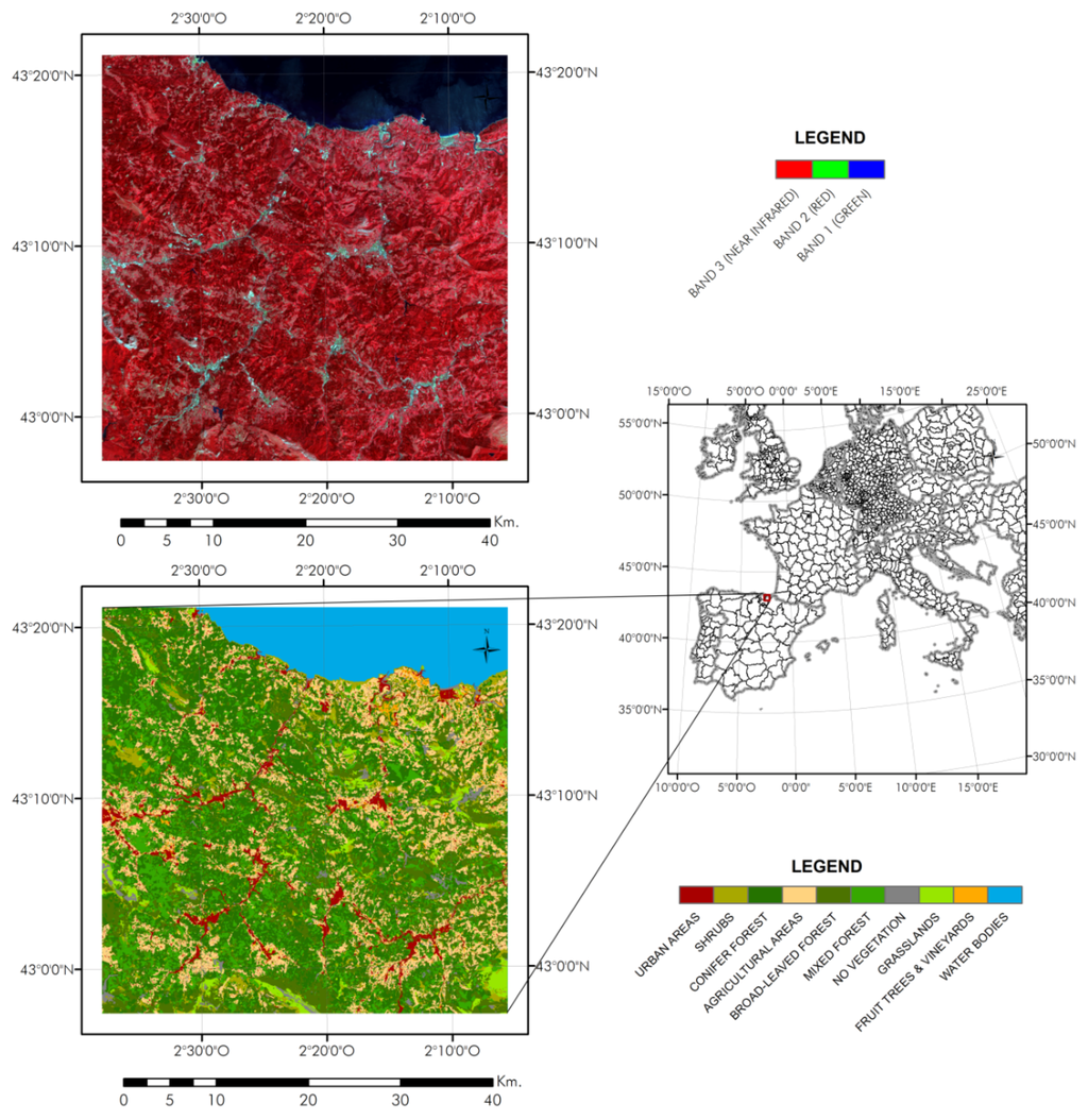
Figure 1.
Land cover information (level 3) and SPOT 5 scene of the study site.
Figure 1.
Land cover information (level 3) and SPOT 5 scene of the study site.

2.2. Data Acquisition and Processing
A SPOT 5 scene acquired the 30 August 2008 at 11:11 UTC time was orthorectified and converted from digital numbers (DN) to top of atmosphere radiance (TOARD), in W·m−2·sr−1·μm−1 units, by using the gain and offset values provided in the metadata for each spectral band. Afterwards, TOARD was converted to ground reflectance (ρt) including atmospheric correction based on dark object subtraction method [35]. The study site had an extent of 44 × 44 km, extracted from a SPOT 5 scene with a spatial resolution of 10 m and four spectral bands, i.e., green: 0.50–0.59 µm, red: 0.61–0.68 µm, NIR (near infrared): 0.78–0.89 µm and SWIR (short-wave infrared): 1.58–1.75 µm. The solar angles at the time of acquisition (i.e., solar elevation = 53.53°, solar azimuth = 155.02) are typical of an end of summer scene, when topographic effect is not that severe, but it still leads to interpretation errors unless efficiently removed. Moreover, this date was selected as most RS applications use images acquired in summer months.
2.3. Ancillary Information
The land cover (LC) information was obtained from the local cartography of vegetation and land use of the region of Basque Country [36] of 2005 (see Figure 1). This cartographic product has a Minimum Mapping Unit of 0.25 Ha, a scale of 1:10.000, and a legend of 235 units, subsequently reclassified in 2 (level 1), 4 (level 2) and 8 (level 3) broad land cover classes. The area is heterogeneous and can be deemed representative of the most common land cover classes in Spain and Europe, especially in mountainous areas. For instance, six out of the eight most common land cover classes in Spain were present in the study area, while the other two (i.e., non-irrigated arable land and complex cultivation patterns) are not frequent in mountainous areas. The study area is covered in more than 60% by forest and pastures (within agricultural areas), but other land covers such as shrubs, sclerophyllous vegetation, moors or bare soil (no vegetation) have a predominant coverage within the study site. Besides, more than 10% of the area is covered by water bodies that have been masked out in this work. On the other hand, NDVI was obtained from the ground reflectance obtained from the SPOT 5 scene. More than 80% of the pixels correspond to NDVI values higher than 0.6.
As seen in Table 2, fruit trees, vineyards, agricultural areas and pastures are characterized by lower variance of cosγi as they are mostly located on gentler slopes. The lower mean value and higher variance of cosγi correspond to broad-leaved forest and open spaces with little or no vegetation, including rocks and bare soil, typical from mountainous areas.
Table 2.
Area of each land cover type and statistics of each cosγi for each stratum.
| LC | % | Min | Max | Mean | SD |
|---|---|---|---|---|---|
| Artificial surfaces | 3.70 | MASKED | |||
| Agricultural areas (pastures) | 15.48 | 0.014 | 1.000 | 0.783 | 0.123 |
| Broad-leaved forest | 18.52 | 0.002 | 1.000 | 0.676 | 0.192 |
| Coniferous forest | 26.66 | 0.002 | 1.000 | 0.723 | 0.178 |
| Mixed forest | 13.90 | 0.001 | 1.000 | 0.719 | 0.175 |
| Natural grasslands | 2.54 | 0.003 | 1.000 | 0.758 | 0.167 |
| Shrubs, moors and heathland | 4.58 | 0.005 | 1.000 | 0.744 | 0.174 |
| Fruit-trees, vineyards | 1.27 | 0.096 | 1.000 | 0.791 | 0.118 |
| Open spaces with little or no vegetation | 2.04 | 0.002 | 1.000 | 0.707 | 0.195 |
| Water bodies (+ wetlands) | 11.31 | MASKED | |||
The characteristics of topography (cosγi) were computed at the original 5 m resolution of the available DEM and then resampled to 10 m applying the bilinear interpolation technique to have the same spatial resolution of SPOT 5 images. The DEM, provided by the Spanish National Geographic Institute (IGN), was obtained by interpolation from LIDAR flights of the National Aerial Orthophotography Plan (PNOA) [37]. The nominal density and elevation accuracy of the LIDAR data were 0.5 points/m2 and 0.2 m, respectively.
2.4. Stratification Strategies
The information provided by local cartography and NDVI data was used to generate land cover strata following different strategies (Table 3). Six different stratification approaches were considered and compared with the traditional non-stratified approach. On the one hand, the LC cartography was reclassified in 2, 4 and 8 strata, while flat areas, cast shadows, water bodies and wetlands, and artificial surfaces were masked out. On the other hand, arbitrary NDVI thresholds were used [16,28], to split the scene in 2, 4 and 8 strata, masking again flat areas and cast shadows, as well as pixels where NDVI < 0.
Table 3.
Stratification approaches.
| Approach | Number of Strata | Land Cover | Code | Coverage (%) | Masked |
|---|---|---|---|---|---|
| NO-STRAT. | 1 | All land covers | ALL | 100.00 | - |
| LC-2 | 2 | Artificial surfaces | ARTIF | 3.70 | YES |
| Non forested areas | NOFOREST | 25.91 | NO | ||
| Forested areas | FOREST | 59.08 | NO | ||
| Water bodies | WATER | 11.31 | YES | ||
| LC-4 | 4 | Artificial surfaces | ARTIF | 3.70 | YES |
| Agricultural areas (pastures) | AGRIC-4C | 15.48 | NO | ||
| Forested areas | FOREST | 59.08 | NO | ||
| Shrubs, moors, heathlands | SHRUB | 4.58 | NO | ||
| Grasslands, bare soil and rocks | OTHER | 5.85 | NO | ||
| Water bodies (+ wetlands) | WATER | 11.31 | YES | ||
| LC-8 | 8 | Artificial surfaces | ARTIF | 3.70 | YES |
| Agricultural areas (pastures) | AGRIC-8C | 15.48 | NO | ||
| Broad-leaved forest | BROAD | 18.52 | NO | ||
| Coniferous forest | CONIF | 26.66 | NO | ||
| Mixed forest | MIXED | 13.90 | NO | ||
| Natural grasslands | GRASS | 2.54 | NO | ||
| Shrubs, moors and heathland | SHRUB | 4.58 | NO | ||
| Fruit-trees, vineyards | FRUIT | 1.27 | NO | ||
| Open spaces with little or no vegetation | NOVEGET | 2.04 | NO | ||
| Water bodies (+ wetlands) | WATER | 11.31 | YES | ||
| NDVI-2 | 2 | 0 < NDVI < 0.4 | NDVI 0-4 | 13.30 | NO |
| 0.4 < NDVI < 1 | NDVI 4-1 | 86.70 | NO | ||
| NDVI-4 | 4 | 0 < NDVI < 0.4 | NDVI 0-4 | 13.30 | NO |
| 0.4 < NDVI < 0.6 | NDVI 4-6 | 5.91 | NO | ||
| 0.6 < NDVI < 0.8 | NDVI 6-8 | 23.32 | NO | ||
| 0.8 < NDVI < 1 | NDVI 8-1 | 57.47 | NO | ||
| NDVI-8 | 8 | 0 < NDVI < 0.2 | NDVI 0-2 | 4.54 | NO |
| 0.2 < NDVI < 0.4 | NDVI 2-4 | 8.77 | NO | ||
| 0.4 < NDVI < 0.5 | NDVI 4-5 | 2.50 | NO | ||
| 0.5 < NDVI < 0.6 | NDVI 5-6 | 3.40 | NO | ||
| 0.6 < NDVI < 0.7 | NDVI 6-7 | 7.32 | NO | ||
| 0.7 < NDVI < 0.8 | NDVI 7-8 | 16.00 | NO | ||
| 0.8 < NDVI < 0.9 | NDVI 8-9 | 55.32 | NO | ||
| 0.9 < NDVI < 1 | NDVI 9-1 | 2.15 | NO |
2.5. Selected Topographic Correction Algorithms
SCS + C (1) and SE (2) methods were selected to correct the topographic effect both in the non-stratified and the stratified approaches. The former was originally proposed by Soenen et al. [12] as a modification of the SCS algorithm previously designed by Gu and Gillespie [38], showing a good performance on different evaluations of TOC methods [15,39]. Moreover, this algorithm was originally designed for forested areas, which are predominant on tilted slopes where the topographic effect is more severe. On the other hand, SE method was also selected as it was previously tested on stratified approaches with satisfactory results [15,16]. This method was originally proposed by Teillet et al. [10] and it is based on the linear regression between the reflectance of each stratum for the considered spectral band and the solar illumination, that is, the cosine of solar incidence angle:
where ρSCSC,λ and ρSE,λ are the SCS + C-corrected and SE-corrected ground reflectance of band λ, respectively, ρλ is the ground reflectance of band λ in rugged terrain, β is the terrain slope computed from the DEM, is the solar zenith angle, cλ the empirical coefficient of band λ, calculated as the ratio between the intercept (A) and the slope (B) of the regression of cosγi against the reflectance of each band, and is the mean ground reflectance of band λ in rugged terrain. Flat pixels (i.e., β < 5°), cast shadowed pixels and self-shadowed pixels, (i.e., pixels where cosγi < 0), were masked out and excluded from the calculation of the linear regressions used in both methods. cλ was calculated from every pixel of each stratum except for masked pixels.
2.6. Evaluation Strategies
The performance of the different stratification types tested needs to be evaluated using objective strategies. Different evaluation strategies have been proposed in the literature and seven of them were used in this study: Visual analysis, analysis of correction parameters, correlation analysis, radiometry stability of land covers, intraclass variance reduction, comparison of reflectance between sunlit and shaded slopes, and evaluation using synthetic images.
2.6.1. Visual Analysis
The first indicator of the quality of TOC correction is the visual analysis of the corrected image, but this subjective criterion must be combined with a quantitative assessment. Minor differences between corrections could be hardly noticed, and the results depend on the skills of the observer.
2.6.2. Analysis of Correction Parameters
As explained above, SE and SCS + C methods are both based on the regression between the spectral reflectance of land cover classes and cosγi. The coefficient of correlation of the fitted regression illustrates the robustness and reliability of the TOC correction. Therefore, it is interesting to evaluate this correlation and also how values change for each stratum when different stratification strategies are applied. Moreover, cλ parameter of SCS + C correction is obtained as the quotient between intercept and slope of the mentioned linear regression and its values for each land cover and spectral band are analyzed. In order to help interpret these values, the standard deviation (SD) of cosγi for each stratum was also considered, as it might impact the regressions fitted.
2.6.3. Correlation Analysis
Probably the most used criteria to evaluate the performance of TOC correction is the correlation of cosγi against the reflectance of each spectral band after the correction [3,19,40,41]. In general, the higher the reduction of this correlation, the better the performance of the TOC algorithm. This was measured through the correlation coefficient (r) of the linear regression between cosγi and the TOC corrected reflectance.
2.6.4. Radiometric Stability of Land Covers
Ideally, the original median reflectance of each land cover should not change after TOC correction; otherwise the TOC method would have introduced a bias [14,15]. Strictly speaking, this should not be considered a criterion to assess the performance of the correction, but a measure of its stability. In this work, the stability was assessed by splitting the image in the eight land cover classes of LC-8 (masking water, wetlands and artificial surfaces) and comparing the median of each class before and after TOC correction.
2.6.5. Intraclass Variance Reduction
A widely used procedure to evaluate the performance of TOC algorithms is to measure the reduction of intraclass variance after correction. Ideally, TOC correction should result in more homogeneous land covers, (i.e., independent of illumination, aspect or slope). For that purpose, instead of the commonly used SD [3,5,42], the inter quartile range (IQR) was used in this work. IQR measures the difference between quartile 3 (Q3) and quartile 1 (Q1) for each land cover, and it is less sensitive to outliers than SD. For each land cover the IQR was calculated before and after the correction, and subsequently the area weighted IQR average was calculated.
2.6.6. Comparison of Reflectance between Sunlit and Shaded Slopes
In the study area, coniferous forests take the steepest slopes, and thus are particularly affected by the topographic effect. A successful TOC correction should reduce the differences in radiometry between forests located on sunlit and shaded slopes [43]. Two random samples of 1000 pixels of coniferous forest were extracted from sunlit and shaded slopes, respectively. Then, the reflectance difference between these two samples was computed before and after TOC correction. Ideally, pixels of the same land cover class should be more homogeneous after the correction, with reflectance difference values close to zero.
2.6.7. Evaluation Using Synthetic Images
Synthetic images can be used to evaluate topographic correction algorithms by comparing a TOC corrected scene with a synthetic image generated assuming a completely flat topography and considered an ideal reference [4,44]. In this study, synthetic images were generated for the same acquisition time and study area of the SPOT 5 image using the model developed in [4,44], and then TOC corrected Synthetic Real (SR) images were compared with the Synthetic Horizontal (SH) reference. This comparison was quantitatively carried out by calculating the Mean Structural SIMilarity index (MSSIM) [45], which measures how similar two scenes are according to three different components: luminance, structure and contrast comparison.
3. Results
3.1. Visual Analysis
The visual analysis of the TOC and STOC approaches suggest a successful removal of the topographic effect over the vast majority of the study site regardless of the stratification option and TOC method. Differences between traditional and stratified corrections were minor. While shadowed slopes in mountainous areas, mainly covered by forest, grasslands, shrubs and bare soil were topographically corrected, flat areas, water bodies and artificial surfaces remained uncorrected as they were masked out. Similarly, agricultural areas, frequently located on gentler slopes, were not strongly affected by topography. A detail zone of the scene is shown in Figure 2 for further information.
The detail zone in Figure 2 corresponds to an extremely abrupt topography mainly covered by broad-leaved and conifer forests, pastures and bare soil. The area is a good example of the limits of semi-empirical corrections, unable to fully correct shadowed areas where no direct irradiance is impinging on the surface [14]. All in all, the traditional SCS + C and SE correction (see Figure 2b,c) performed adequately in the vast majority of the area, while LC-8 and NDVI-8 stratification approaches (see Figure 2d–g) were visually very similar to the traditional correction. Figure 2 also shows areas where shaded slopes had been slightly overcorrected (see areas labelled as A). This effect was less apparent in LC-8 approach (labelled as B).
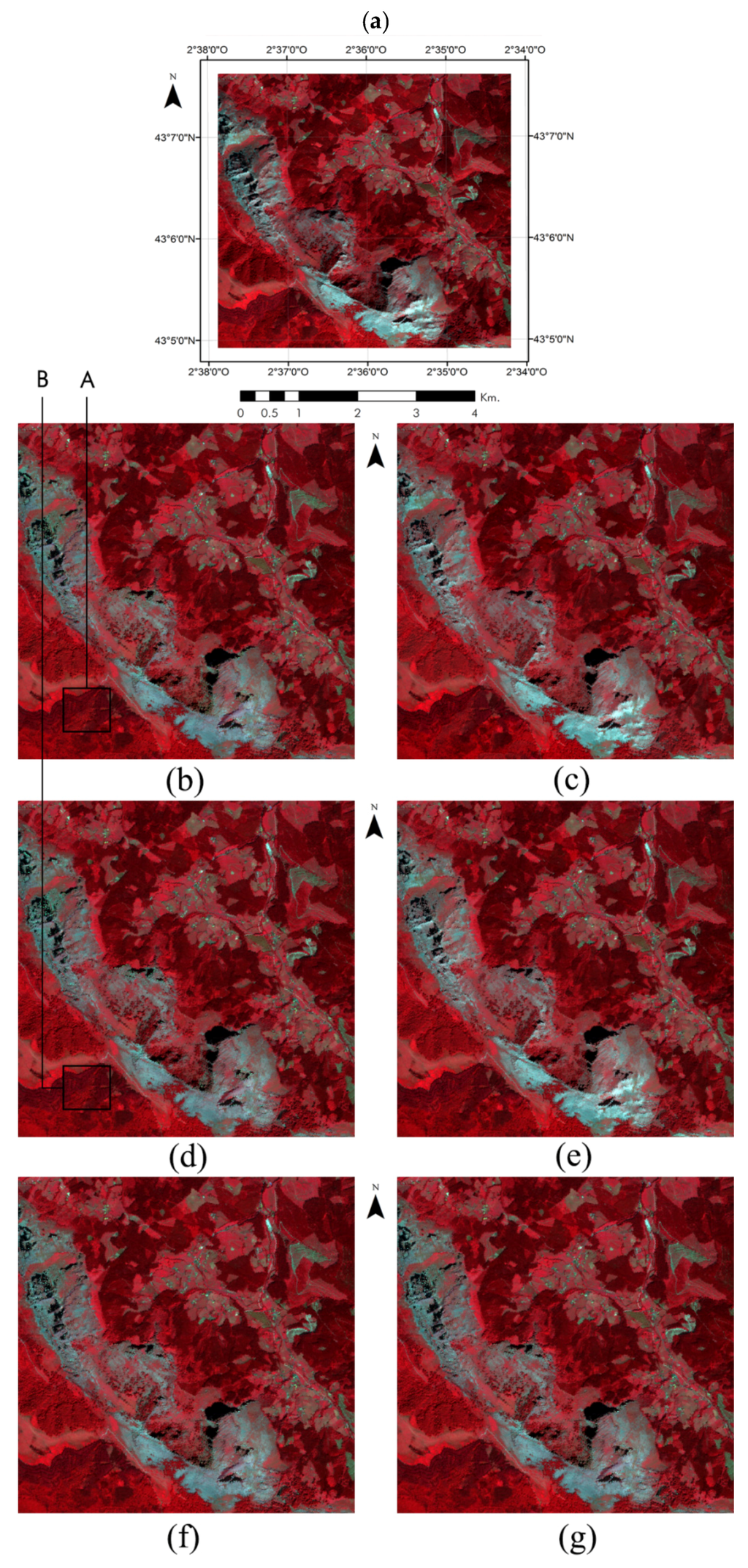
Figure 2.
Detail zone with (a) Uncorrected scene; (b) SCS+C-corrected scene with no stratification; (c) SE-corrected scene with no stratification; (d) SCS+C-corrected scene with LC-8 stratification; (e) SE-corrected scene with LC-8 stratification; (f) SCS+C-corrected scene with NDVI-8 stratification; (g) SE-corrected scene with NDVI-8 stratification.

3.2. Analysis of Correction Parameters
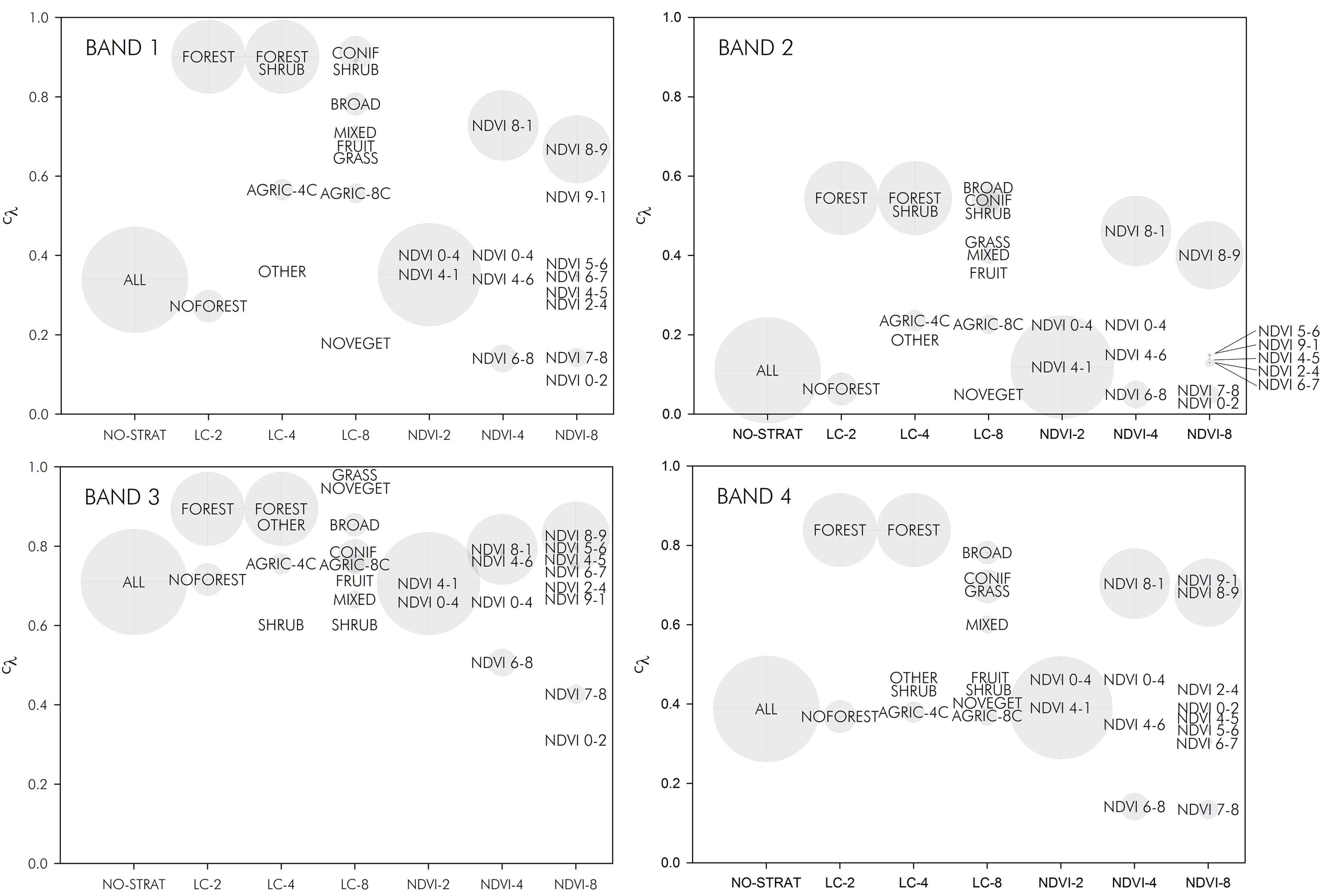
In Figure 3, the cλ values obtained for each stratum and spectral band of the image are displayed. There were great differences for this value when the traditional, non-stratified approach was compared with the different stratifications. In general, parameter cλ was higher for high NDVI values (i.e., NDVI > 0.8) and forested land covers.
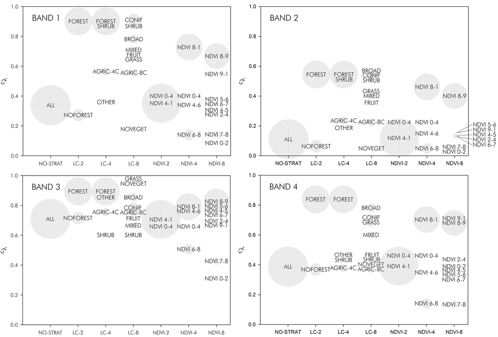
Figure 3.
cλ coefficient obtained for each spectral band on the different stratification approaches evaluated. Circle sizes represent the proportion of each stratum in the study area.
Figure 3.
cλ coefficient obtained for each spectral band on the different stratification approaches evaluated. Circle sizes represent the proportion of each stratum in the study area.
In Figure 4, the correlation between cosγi and the reflectance of spectral bands (for each land cover) is depicted. This correlation is a key factor of both SE and SCS + C corrections. Although r values did not change dramatically in the different stratifications tested, in bands 1 and 2 there was a clear trend of higher correlation for NDVI-based stratifications, with higher r values for every NDVI strata compared with the non-stratified approach. In these two bands, the lowest correlation among the NDVI strata was achieved by the NDVI 9-1 strata, but it was still higher than the correlation for the non-stratified option. LC-based stratifications led to minor changes in correlation when only two strata were considered and also with four strata. In both cases, FOREST obtained the highest correlation. When eight strata were considered, BROAD led to improved correlations but the rest obtained similar or lower correlations.
For bands 3 and 4, different trends were obtained for the different stratification options evaluated (Figure 4). In band 3, the non-stratified option already yielded quite a high r value that then increased or decreased after stratification depending on the particular NDVI or LC class considered. Generally, NDVI strata with moderate-high NDVI values (>0.4) yielded higher r values. In band 4, after stratification, r values did not change significantly in most cases, but in some LC (BROAD, SHRUB, GRASS, AGRIC-4C, OTHER, AGRIC-8C, NOVEGET, FRUIT) and NDVI classes (NDVI 4–6, NDVI 6–8, etc.) r value increased.
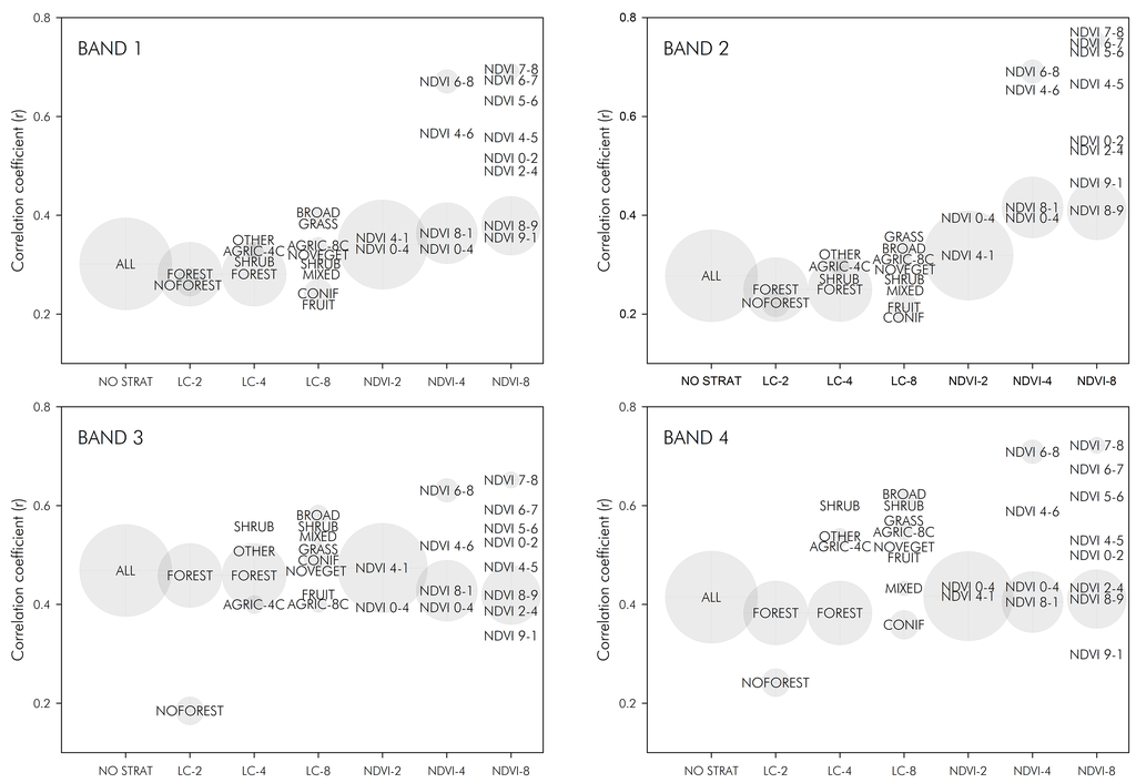
Figure 4.
Correlation coefficient between cosγi and the reflectance of spectral bands for each stratum. Circle sizes represent the proportion of each stratum in the study area.
Figure 4.
Correlation coefficient between cosγi and the reflectance of spectral bands for each stratum. Circle sizes represent the proportion of each stratum in the study area.

In Figure 5, the SD of cosγi is displayed for each stratum in every stratification approach. This figure showed AGRIC-4C, AGRIC-8C, FRUIT AND NDVI 9-1 strata had lower SD, as these were located in gentler slopes characterized by more homogeneous topography (i.e., a higher range of cosγi values were centered around the median). This could explain the lower correlation depicted in Figure 4, especially in band 3. The results in other LC strata were not so clear, probably because their SD values were very similar to the non-stratified case.
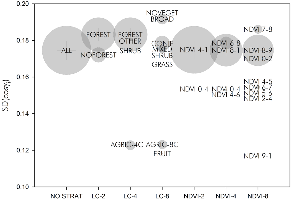
Figure 5.
SD of cosγi for each stratum. Circle sizes represent the proportion of each stratum in the study area.
Figure 5.
SD of cosγi for each stratum. Circle sizes represent the proportion of each stratum in the study area.

3.3. Correlation Analysis
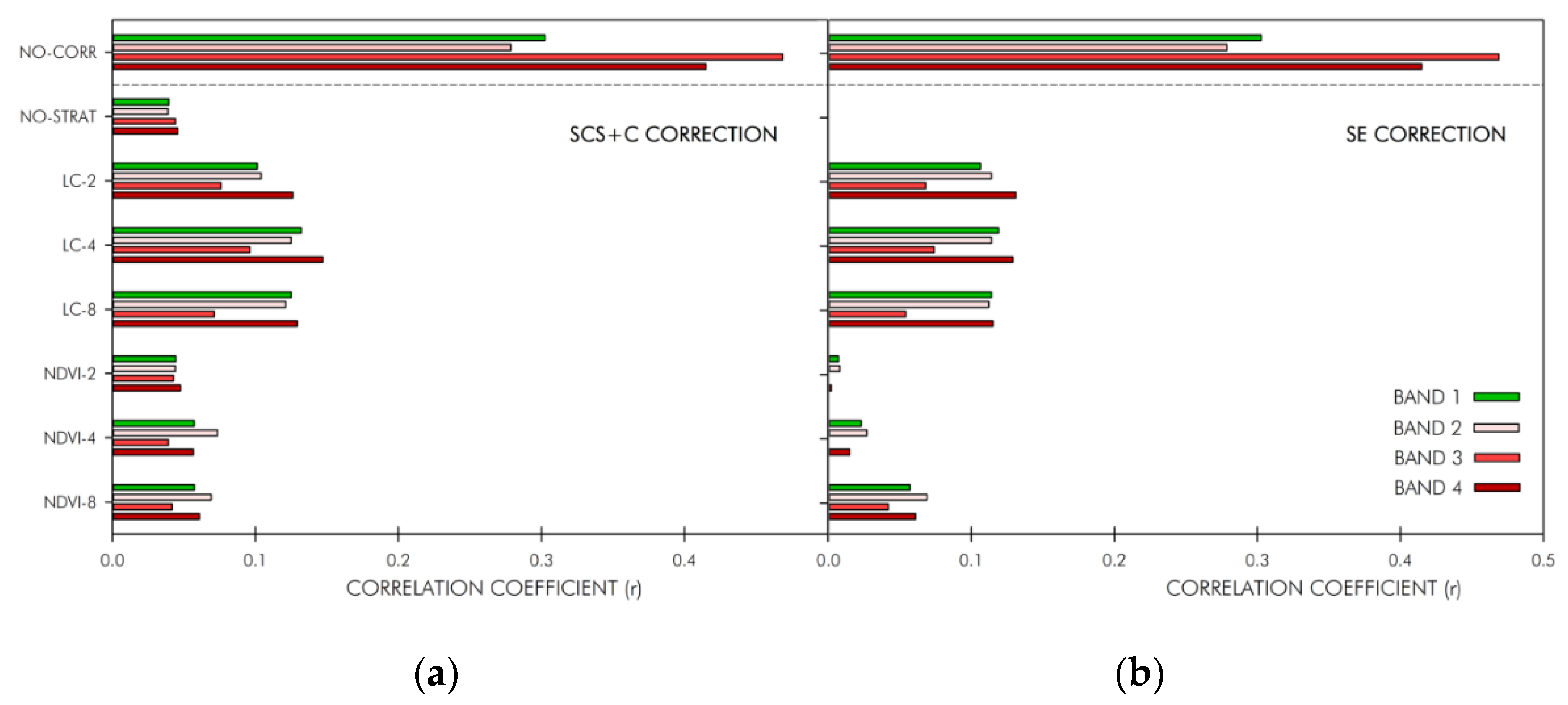
In Figure 6, the correlation coefficient of the regression between cosγi and the reflectance of each spectral band are shown for the uncorrected image (top) and then for the traditional and stratified TOC-corrected images. In the uncorrected image, r ranged from 0.25 to 0.50, being higher in the infrared bands (i.e., b3 and b4). All TOC corrections were successful in removing this correlation to a certain extent in all the bands. Notwithstanding that, all the topographic corrections showed slightly positive values of residual correlation (except for the non-stratified SE correction, that showed an r = 0 for all the bands due to its mathematical definition), proof of an incomplete removal of the topographic effect. All in all, these low values (i.e., r < 0.1) are not significant if compared to the r values of the uncorrected image. According to this evaluation criterion, there was not a clear improvement of the correction when stratification was applied. Furthermore, in the case of SCS + C the LC-based stratification approaches performed slightly worse (higher correlation) than the non-stratified option, while minor differences were observed between the NDVI-based stratifications and the non-stratified TOC. Alternatively, SE showed a similar trend, but NDVI-based approaches had slightly lower r values if compared with SCS + C correction.
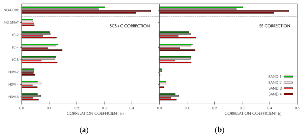
Figure 6.
Correlation coefficient of the regression between cosγi and the reflectance of each spectral band for the uncorrected image (NO-CORR.) and the different strategies tested on SCS + C correction (a) and SE correction (b).
Figure 6.
Correlation coefficient of the regression between cosγi and the reflectance of each spectral band for the uncorrected image (NO-CORR.) and the different strategies tested on SCS + C correction (a) and SE correction (b).
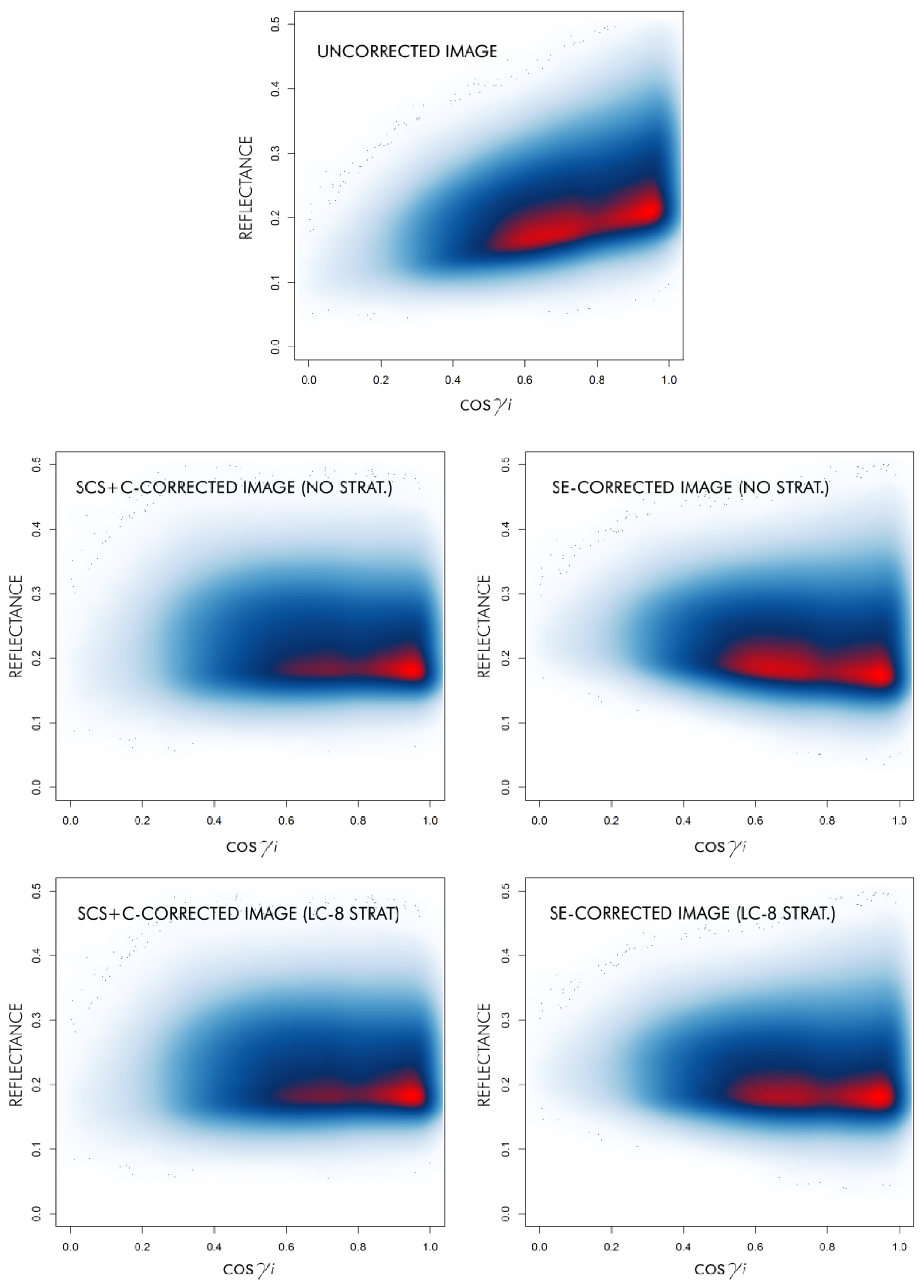
This significant decrease in the correlation between cosγi and the reflectance of each spectral band is clearly observed in Figure 7, regardless of the stratification approach or tested TOC method. The topographic effect on near infrared reflectance (band 3) of forest pixels is clearly observed in the figure (on top), with high values of reflectance associated with cosγi values close to 1. This dependence of reflectance on illumination was successfully removed with non-stratified TOC corrections. SE correction showed a slight overcorrection, which seems to be solved by the stratified SE correction. These results are in line with the findings of Figure 6, showing a successful removal of the topographic effect in infrared bands.
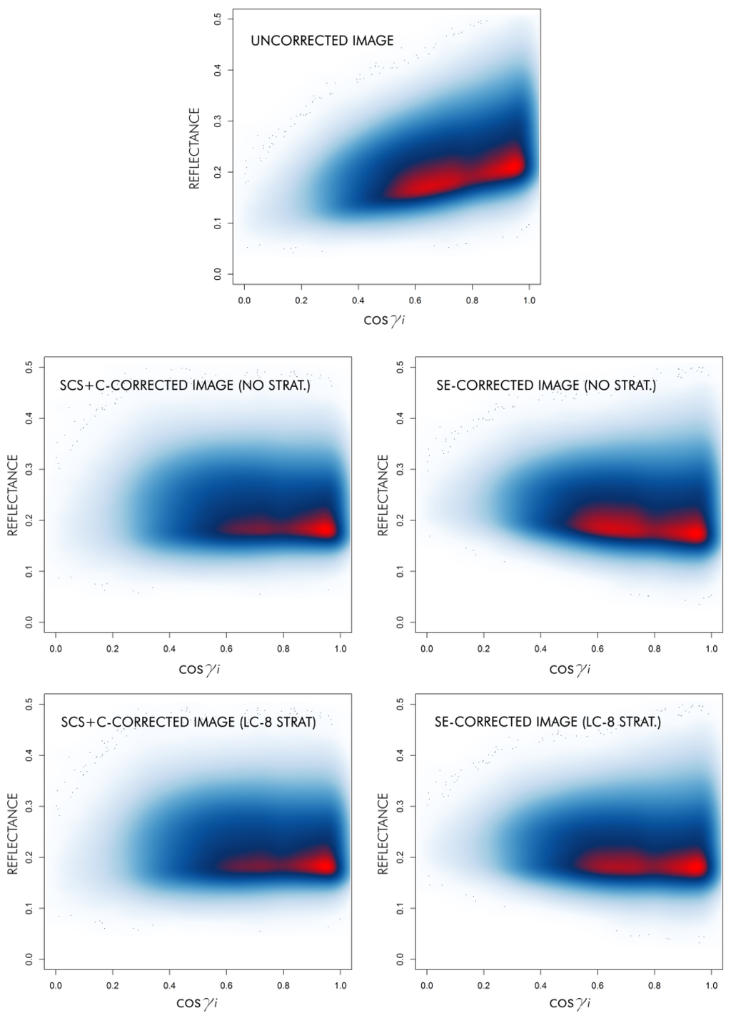
Figure 7.
Scatterplot of the spectral reflectance of band 3 (NIR) for forest strata versus the cosine of solar incidence angle.
Figure 7.
Scatterplot of the spectral reflectance of band 3 (NIR) for forest strata versus the cosine of solar incidence angle.
3.4. Radiometric Stability of Land Covers
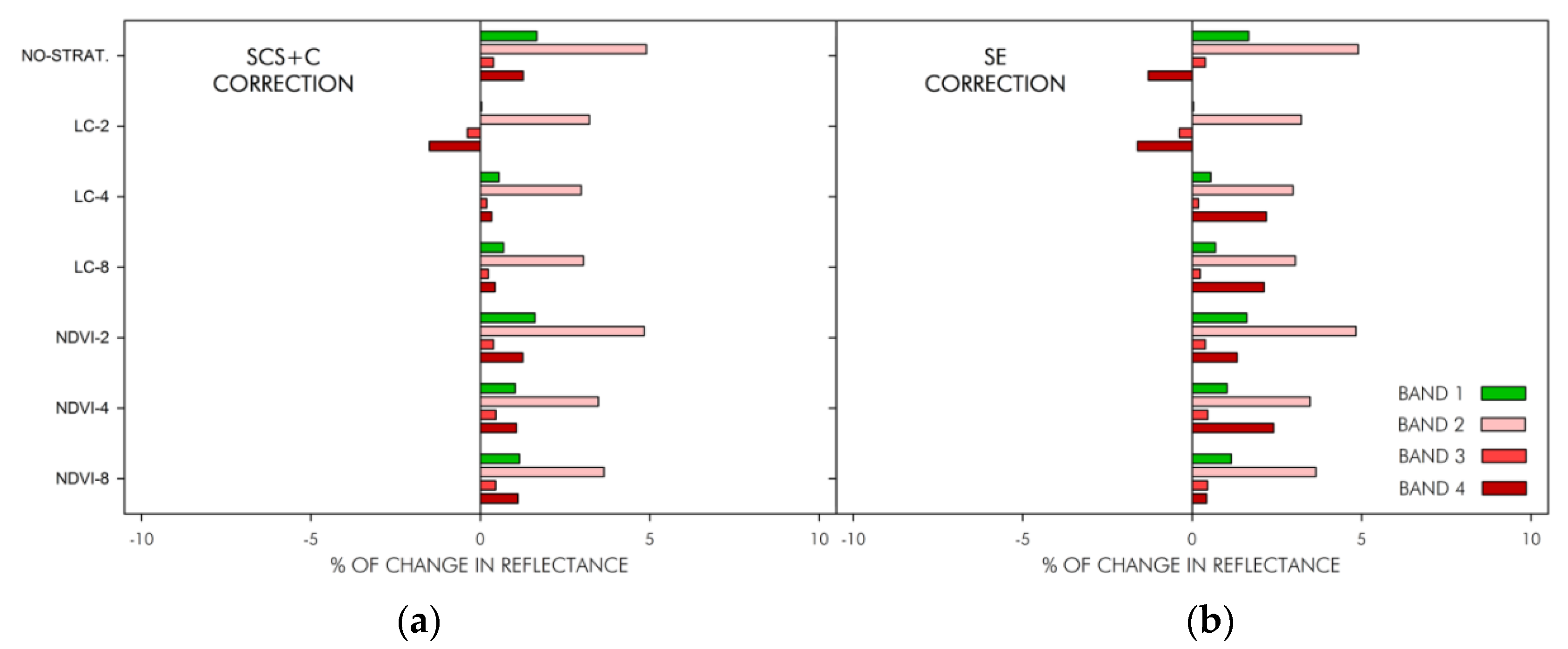
In Figure 8, the area weighted average of the relative difference of land covers’ median reflectance before and after TOC correction is shown, comparing corrected and uncorrected scenes band-wise. The figure shows a clear increase in the uncorrected median reflectance of land covers in all the bands after SCS + C and SE corrections were applied, except for infrared bands in LC-2. This bias was consistent and very similar when different stratification approaches were compared, although its magnitude suggests it to be negligible.

Figure 8.
Radiometric stability of land covers represented by the area-weighted average of % change in land cover reflectance after SCS+C correction (a) and SE correction (b).
Figure 8.
Radiometric stability of land covers represented by the area-weighted average of % change in land cover reflectance after SCS+C correction (a) and SE correction (b).
3.5. Intraclass Variance Reduction
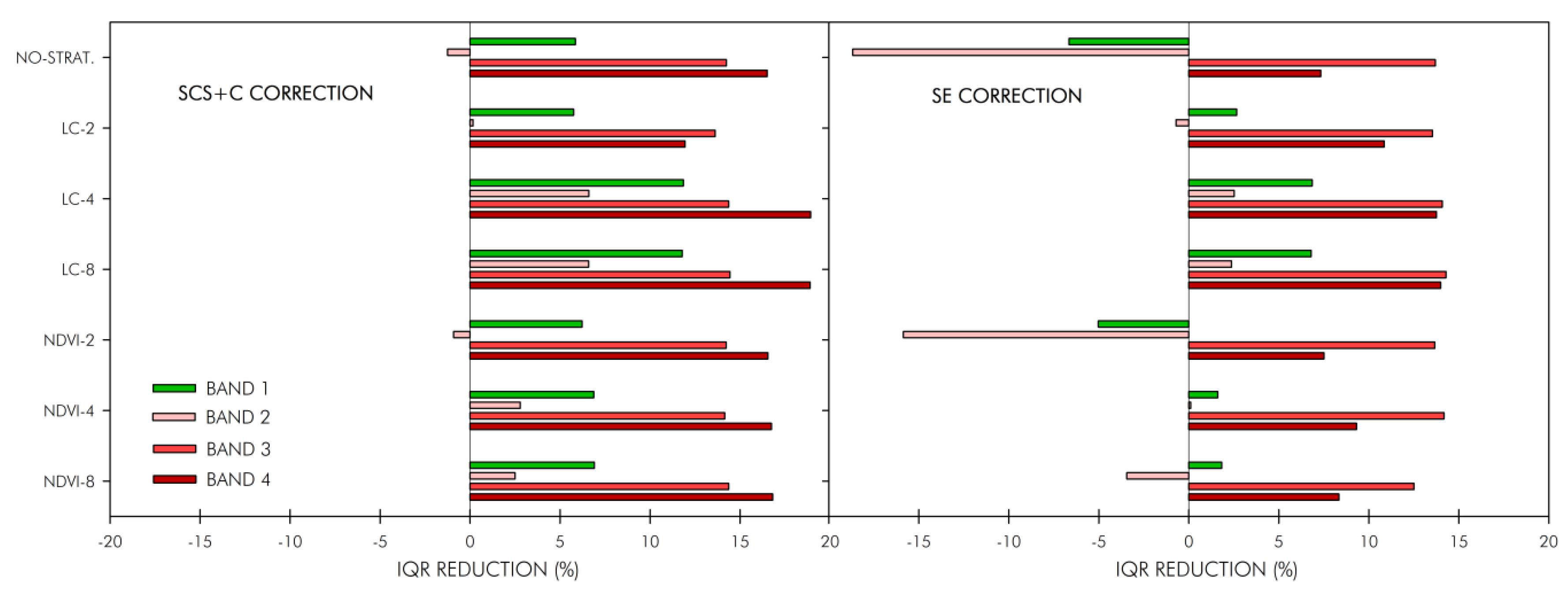
In Figure 9, the IQR reduction of land covers’ reflectance performed by each correction is shown. IQR reduction was higher for infrared bands (i.e., bands 3 and 4). This can be explained by the higher influence of the topographic effect on these bands, demonstrated by the higher correlation between cosγi and reflectance for these bands (see Figure 4). On the contrary, in some cases, visible bands (i.e., bands 1 and 2) showed a negative reduction of IQR, that is, an increase of reflectance variance compared to the uncorrected image. This effect was particularly distinct in the case of non-stratified SE correction, but this issue was solved by most of the stratification approaches. Small differences were observed between stratification approaches in the SCS+C case. Figure 9 shows that stratification did not significantly improve the IQR reduction rate achieved by the non-stratified correction in infrared bands. On the contrary, some improvements were observed in bands 1 and 2 for the LC-based stratifications, but differences with the other configurations were not that marked.
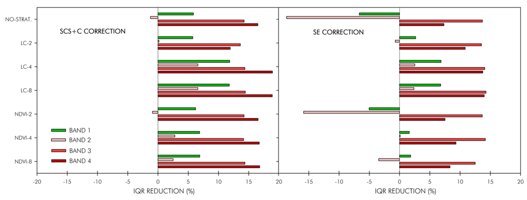
Figure 9.
Mean intraclass IQR reduction. Measured as the area-weighted average of IQR reduction for eight land covers.
Figure 9.
Mean intraclass IQR reduction. Measured as the area-weighted average of IQR reduction for eight land covers.
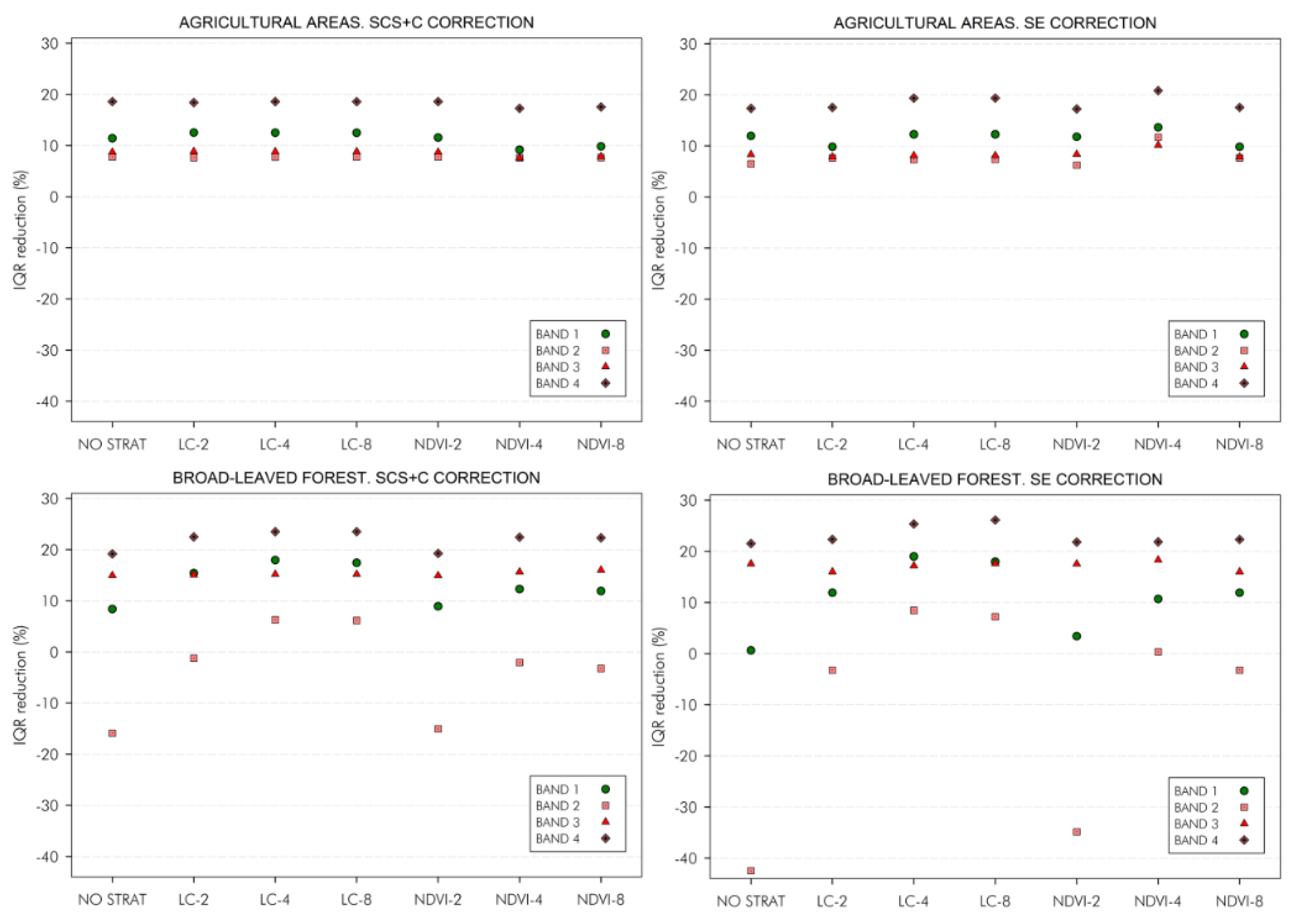
If the results showed in Figure 9 are analyzed by land cover, additional information is obtained. For instance, in the non-stratified option, broad-leaved forests (see Figure 10) showed a greater reduction of IQR of infrared bands (up to 15%–20%) than in general (Figure 9). This means that this land cover was particularly homogenized after TOC correction, regardless of the tested TOC method. Besides, this reduction significantly increased for the different stratification approaches of SCS+C and SE, especially the LC-based ones. In fact, the higher the number of strata considered the better. On the contrary, both methods failed to reduce the IQR in broad-leaved forests in band 2 when they were applied in a non-stratified way, but the stratification approaches (except for NDVI-2, with similar results to the non-stratified option) partially solved this problem.
On the other hand, agricultural areas (pastures in a vast majority) were less affected by the topography (i.e., low SD(cosγi)) and had low correlation between cosγi and reflectance (Figure 4 and Figure 5). This land cover showed a slightly lower IQR reduction, and differences among stratification approaches were inappreciable and clearly not significant.
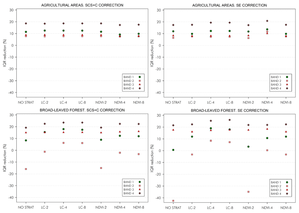
Figure 10.
Intraclass IQR reduction of broad-leaved forest and agricultural areas for each spectral band.
Figure 10.
Intraclass IQR reduction of broad-leaved forest and agricultural areas for each spectral band.
3.6. Comparison of Reflectance between Sunlit and Shaded Slopes
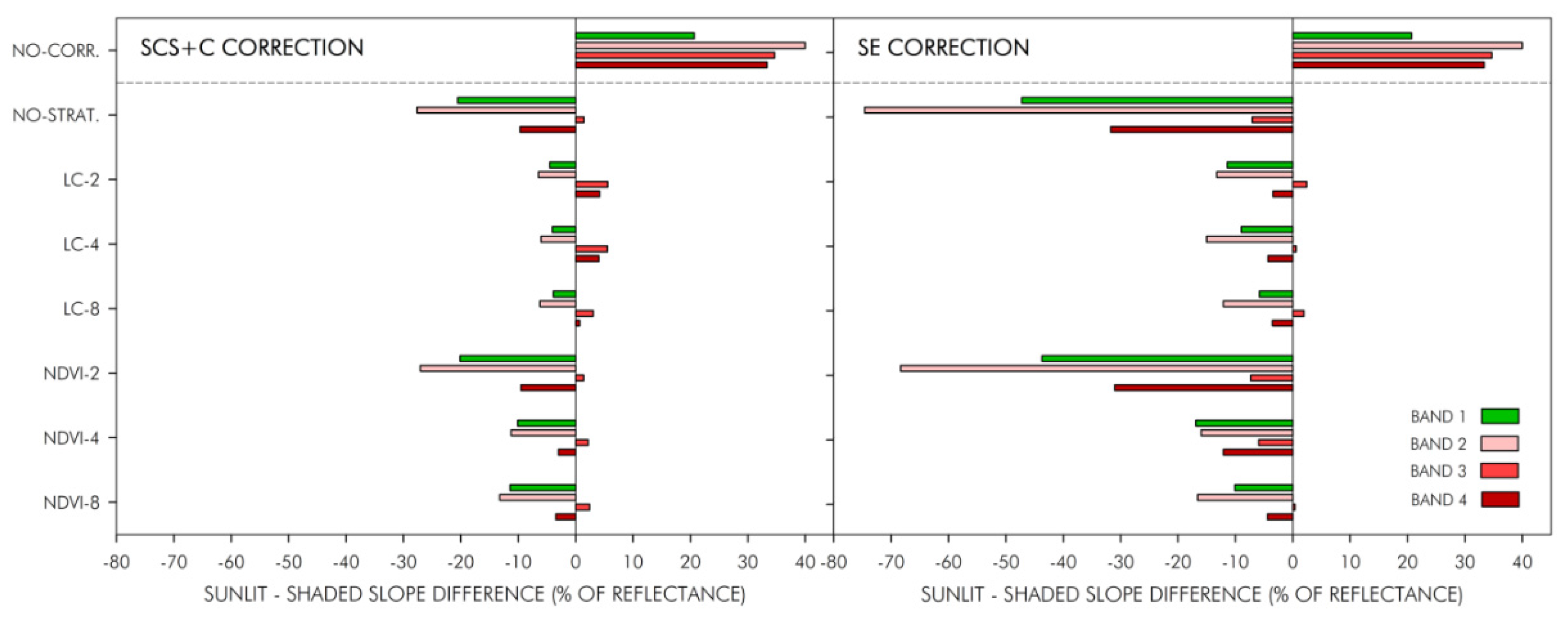
When the uncorrected scene was analyzed, the reflectance difference between pixels of conifer forests located on sunlit slopes (facing the sun) and shaded slopes (facing away from the sun) was up to 30%–40% due to the topographic effect (see Figure 11). Among spectral bands, this difference was again higher for infrared bands. After the correction, this positive difference between sunlit and shaded slopes was completely removed in most of the stratification approaches (except for some cases in b3 and b4 with SCS+C correction), and what is more, a systematic overcorrection was observed mostly in visible bands (i.e., b1 and b2). This effect was clear in both non-stratified corrections (but clearly higher in the case of SE) and it was also apparent in the forested areas of the detail zone in Figure 2b. Overcorrection was not that strong in the LC-based stratifications, particularly in LC-4 and LC-8. However, NDVI based stratifications, and in particular, NDVI-2 led to strong overcorrection in this land cover.

Figure 11.
Reflectance difference between sunlit and shaded slopes for conifer forests.
Figure 11.
Reflectance difference between sunlit and shaded slopes for conifer forests.
3.7. Evaluation Using Synthetic Images
The results obtained with this technique are shown in Table 4, where MSSIM values are depicted for each case. Higher MSSIM values correspond to a closer match between the TOC corrected scene and the ideal reference (SH), and thus to a better reduction of the topographic effect. The MSSIM value for the uncorrected (NO-CORR.) image is also depicted in Table 4 as a reference for interpreting the other cases.
Table 4.
MSSIM of the different stratification approaches for each band. Ranks from 0 (worst) to 1 (best).
| TOC | SCS+C | SE | ||||||
|---|---|---|---|---|---|---|---|---|
| STRAT. | b1 | b2 | b3 | b4 | b1 | b2 | b3 | b4 |
| NO-CORR. | 0.801 | 0.794 | 0.720 | 0.612 | 0.801 | 0.794 | 0.720 | 0.612 |
| NO-STRAT. | 0.890 | 0.885 | 0.882 | 0.857 | 0.894 | 0.879 | 0.878 | 0.846 |
| LC-2 | 0.807 | 0.792 | 0.790 | 0.742 | 0.816 | 0.798 | 0.789 | 0.748 |
| LC-4 | 0.879 | 0.869 | 0.877 | 0.823 | 0.890 | 0.874 | 0.875 | 0.835 |
| LC-8 | 0.881 | 0.870 | 0.878 | 0.830 | 0.890 | 0.873 | 0.872 | 0.838 |
| NDVI-2 | 0.891 | 0.885 | 0.884 | 0.859 | 0.895 | 0.880 | 0.883 | 0.853 |
| NDVI-4 | 0.872 | 0.868 | 0.882 | 0.840 | 0.871 | 0.861 | 0.872 | 0.801 |
| NDVI-8 | 0.877 | 0.874 | 0.878 | 0.841 | 0.875 | 0.867 | 0.869 | 0.808 |
It is easily observed that all TOCs improved the MSSIM value of the uncorrected scene, and this was particularly true for infrared bands. Among the different stratification approaches tested, LC-2 approach performed slightly worse than other options. Nevertheless, differences in MSSIM were minor, and in fact, none of them improved significantly the correction in comparison to the non-stratified approach. If both methods are compared, slight differences are observed. While SCS+C performed somewhat better in the non-stratified option and NDVI-based stratifications, SE showed slightly higher MSSIM values in LC-based approaches.
4. Discussion
The analysis of correction parameters (cλ) showed similar values to those obtained by Ediriweera et al. [25], who found a considerable variation in cλ depending on the vegetation type. Due to the role of this parameter in the SCS+C method, the higher cλ is, the lesser the effect of the correction. That is, high cλ values soften TOC correction and thus avoid overcorrection on poorly illuminated slopes, commonly reported in the COS and SCS method [12,46]. Pons et al. [47] suggested that this adverse effect could be avoided if pixels under an incidence angle higher than 70° were discarded. Conversely, McDonald et al. [23] found that in flat terrain cλ values obtained for agricultural land covers were very small and consequently CC tended toward a COS correction, while in this study this was only valid in band 4. Although our results are not directly comparable to [23], the same effect is expected on strata with low cλ (i.e., NDVI 6-8 or NDVI 7-8), thus SCS+C tends towards SCS on these cases. Further research on different sampling strategies following [9] would help to analyze how the calculation of cλ, affects the results of topographic correction. In particular, Reese and Olsson [9] concluded that a stratified random sample based on cosγi provided the best TOC and the most stable value of this parameter.
Regarding the degree of correlation between reflectance (or radiance) and cosγi, previous studies reported higher correlations after stratification [6,17]. In our study, this was only true in some cases, depending on the particular land cover and spectral band considered. These results uncovered that, for some particular strata, the cλ values were obtained from regressions fitted with quite low correlations, so TOC correction in these conditions could be unstable. This issue seems to be intrinsic to the stratified approach, and in particular, for strata with a small area in the image either because they are a minority or because a high number of strata is considered. In these cases, it is unlikely that a sufficient variability in cosγi values is guaranteed in each stratum so as to lead to strongly correlated regressions and solid cλ values.
Moreover, all the topographic corrections showed slightly positive values of residual correlation (except for the non-stratified SE correction, that showed an r = 0 for all the bands, due to its mathematical definition), proof of an incomplete removal of the topographic effect, in line with the findings of Gao and Zhang [48]. It must be taken into account that the successful removal of the topographic effect does not necessarily mean r = 0, there could be a residual correlation due to the presence of areas where slope orientation determines the land cover (e.g., Figure 2a).
In terms of radiometric stability of land covers, the observed increase of 1%–5% of the uncorrected median reflectance was already reported by other authors applying the SCS + C method, and also the CC method [15,48], probably due to the formulation of these methods. In a comparable study, Moreira and Valeriano [15] observed that SCS + C correction increased the original radiometry of forests compared to uncorrected data, as the forest samples were mostly located in shaded slopes. On the other hand, similar studies [15,19] observed no significant changes in the mean reflectance of land covers when SE was applied.
The results of intraclass variance reduction per land cover demonstrated a clear improvement of topographic correction of broad-leaved forest when applied in a stratified approach. The reason of this improvement could be a successful identification of this stratum due to the presence of large homogeneous areas of broad-leaved forest.
Finally, the results of the comparison of reflectance between sunlit and shaded are similar to those presented by Ediriweera et al. [25] who observed that SCS + C method seemed to overcorrect reflectance on very steep slopes. This result is in line with the radiometric stability criterion (see Section 3.4), where band 2, and to lesser extent bands 1 and 4, showed a systematic increase in radiometry after correction. Also, the lower correlation values reported in Figure 6 could be partly explained because the non-stratified and the NDVI based stratified options overcorrected some land covers. It should be noted that the NDVI-2 stratification yields very similar values to the non-stratified alternative (in all the different criteria), this could be due to the arbitrary NDVI threshold of 0.4 selected (following [16]), as most of the pixels were located within the NDVI 4-1 strata. A more effective stratification could be based on ISODATA cluster analysis of NDVI, in line with previous studies of other authors [17,18].
To sum up, the visual assessment of the globally applied topographic correction through SCS + C and SE methods revealed a successful removal of the topographic effect. Moreover, the results have been shown to reduce spectral variance of land covers, remove the dependence of reflectance on cosγi, a better balancing between sunlit and shaded slopes and an increase in SSIM indices of every spectral band. Nevertheless, a side effect of this correction is the increase in the mean reflectance of land covers and the slight overcorrection in forested areas. These findings differed from some studies that attributed a poor performance of topographic correction to SCS + C [25]; but were in line with some others [15,39].
The stratification approaches further corrected the topographic effect, improving the performance of the non-stratified option in some evaluation criteria, i.e., IQR reduction of land covers, and removal of the difference between sunlit and shaded slopes. This superior performance was clearer in some particular land covers, such as broad-leaved forest, where LC-based stratification provided much higher IQR reduction. On the contrary, other criteria showed minor improvements when stratified TOC was applied, or even worse performance than the traditional TOC correction (e.g., correlation analysis or evaluation using synthetic images). In the literature, stratified approaches yielded results with varying degrees of success for the respective study site, depending on the stratification strategy, land cover distribution and selected TOC method.
5. Conclusions
After the evaluation of different stratification strategies (based on land cover and NDVI) for two different topographic correction methods and a comparison with their respective non-stratified correction, the results obtained did not show a drastic improvement in the performance of topographic correction when stratification approaches were implemented in this particular case study.
The correlation between the spectral reflectance of land covers and cosγi is particularly important in both topographic correction methods, i.e., Sun-Canopy-Sensor + C and Statistic-Empirical. The empirical coefficient cλ required in the latter clearly changed between the different stratification options and took different values for each strata (in many cases higher than the cλ value obtained for the non-stratified option). However, these cλ variations did not necessarily result from a more robust correlation and issues such as the relative size of the stratum or the variability of cosγi therein played an important role here. In some evaluation criteria, land cover-based stratifications yielded slightly better results than the non-stratified or the NDVI-based stratification options, particularly in the stability of land cover radiometry, intraclass IQR reduction or sunlit-shaded slope difference. The non-stratified and NDVI based stratifications (in particular, NDVI-2) showed a tendency to slightly overcorrect the topographic effect of steep slopes, especially in the case of Statistic-Empirical correction, but this effect was partially removed when land cover-based stratifications were applied.
All in all, even if in some criteria land cover-based approaches performed slightly better than the non-stratified correction, the latter proved to be effective in removing the topographic effect in this study area. This conclusion is deemed important because the non-stratified option can be applied without a priori knowledge or ancillary information about the scene. Furthermore, it can be implemented more easily in automatic image processing chains. Therefore, we suggest that non-stratified topographic correction is considered, due to its good performance and ease of implementation. In any case, future research is necessary on stratification strategies based on a priori unsupervised classifications of the scene to correct, so as to check whether better results are achieved following this approach. Moreover, further studies on different study sites and image acquisition dates are necessary to confirm the conclusions drawn here.
Acknowledgments
The authors gratefully acknowledge the financial support provided by the Public University of Navarre (UPNA). The authors would also like to thank the Spanish National Geographic Institute (IGN) for providing the test data. Part of the research presented in this paper is funded by the Spanish Ministry of Economy and Competitiveness in the frame of the ESP2013-48458-C4-2-P project.
Author Contributions
Ion Sola, María González-Audícana and Jesús Álvarez-Mozos provided the overall conception of this research, designs the methodologies and experiments, and shared equally in the writing of the manuscript; Ion Sola carried out the implementation of proposed algorithms, conducted the experiments and performed the data analyses.
Conflicts of Interest
The authors declare no conflict of interest.
Abbreviations
The following abbreviations are used in this manuscript:
| RS | Remote Sensing |
| DEM | Digital Elevation Model |
| LULC | Land Use/Land Cover |
| LC | Land cover |
| NDVI | Normalized Difference Vegetation Index |
| TOC | TOpographic Correction |
| STOC | Stratified Topographic Correction |
| SE | Statistical-Empirical method |
| SCS+C | Sun-Canopy-Sensor + C |
| CC | C-Correction method |
| COS | Cosine method |
| ICOS | Improved COSine method |
| VECA | Variable Empirical Coefficient Algorithm |
| MM | Modified Minnaert method |
| MIN | MINnaert method |
| EMIN | Enhanced MINmethod |
| EKS | EKStrand method |
| sCC | Smooth C-Correction method |
| 2SN | Two Stage Normalization method |
| SM | Slope Matching Technique |
| UTC | Coordinated Universal Time |
| DN | Digital Number |
| TOARD | Top Of Atmosphere RaDiance |
| IGN | Instituto Geográfico Nacional (Spain) |
| LIDAR | Light detection and ranging |
| PNOA | Plan Nacional de Ortofotografía Aérea (Spain) |
| IQR | Interquartile Range |
| SD | Standard Deviation |
| SH | Synthetic Horizontal image |
| SR | Synthetic Real image |
| MSSIM | Mean Structural SIMilarity Index |
References
- Leprieur, C.E.; Durand, J.M. Influence of topography on forest reflectance using landsat thematic mapper and digital terrain data. Photogramm. Eng. Remote Sens. 1988, 54, 491–496. [Google Scholar]
- Richter, R.; Kellenberger, T.; Kaufmann, H. Comparison of topographic correction methods. Remote Sens. 2009, 1, 184–196. [Google Scholar] [CrossRef]
- Riano, D.; Chuvieco, E.; Salas, J.; Aguado, I. Assessment of different topographic corrections in Landsat-TM data for mapping vegetation types. IEEE Trans. Geosci. Remote Sens. 2003, 41, 1056–1061. [Google Scholar] [CrossRef]
- Sola, I.; González de Audícana, M.; Álvarez-Mozos, J.; Torres, J.L. Synthetic images for evaluating topographic correction algorithms. IEEE Trans. Geosci. Remote Sens. 2014, 52, 1799–1810. [Google Scholar] [CrossRef]
- Lu, D.; Ge, H.; He, S.; Xu, A.; Zhou, G.; Du, H. Pixel-based minnaert correction method for reducing topographic effects on a Landsat 7 ETM+ image. Photogramm. Eng. Remote Sens. 2008, 74, 1343–1350. [Google Scholar]
- Tokola, T.; Sarkeala, J.; Van der Linden, M. Use of topographic correction in Landsat TM-based forest interpretation in Nepal. Int. J. Remote Sens. 2001, 22, 551–563. [Google Scholar] [CrossRef]
- Balthazar, V.; Vanacker, V.; Lambin, E.F. Evaluation and parameterization of ATCOR3 topographic correction method for forest cover mapping in mountain areas. Int. J. Appl. Earth Obs. Geoinf. 2012, 18, 436–450. [Google Scholar] [CrossRef]
- Couturier, S.; Gastellu-Etchegorry, J.P.; Martin, E.; Patiño, P. Building a forward-mode three-dimensional reflectance model for topographic normalization of high-resolution (1–5 m) imagery: Validation phase in a forested environment. IEEE Trans. Geosci. Remote Sens. 2013, 51, 3910–3921. [Google Scholar] [CrossRef]
- Reese, H.; Olsson, H. C-correction of optical satellite data over alpine vegetation areas: A comparison of sampling strategies for determining the empirical c-parameter. Remote Sens. Environ. 2011, 115, 1387–1400. [Google Scholar] [CrossRef]
- Teillet, P.M.; Guindon, B.; Goodenough, D.G. On the slope-aspect correction of multispectral scanner data. Can. J. Remote Sens. 1982, 8, 84–106. [Google Scholar] [CrossRef]
- Smith, J.A.; Lin, T.L.; Ranson, K.J. The lambertian assumption and landsat data. Photogramm. Eng. Remote Sens. 1980, 46, 1183–1189. [Google Scholar]
- Soenen, S.A.; Peddle, D.R.; Coburn, C.A. Scs+c: A modified sun-canopy-sensor topographic correction in forested terrain. IEEE Trans. Geosci. Remote Sens. 2005, 43, 2148–2159. [Google Scholar] [CrossRef]
- Richter, R.; Schläpfer, D. Atmospheric/Topographic Correction for Satellite Imagery; Atcor-2/3 User Guide, Version 9.0.0; ReSe Applications Schläpfer: Wil, Switzerland, 2015; pp. 185–244. [Google Scholar]
- Goslee, S.C. Topographic corrections of satellite data for regional monitoring. Am. Soc. Photogramm. Remote Sens. 2012, 78, 973–981. [Google Scholar] [CrossRef]
- Moreira, E.P.; Valeriano, M.M. Application and evaluation of topographic correction methods to improve land cover mapping using object-based classification. Int. J. Appl. Earth Obs. Geoinf. 2014, 32, 208–217. [Google Scholar] [CrossRef]
- Hantson, S.; Chuvieco, E. Evaluation of different topographic correction methods for Landsat imagery. Int. J. Appl. Earth Obs. Geoinf. 2011, 13, 691–700. [Google Scholar] [CrossRef]
- Bishop, M.P.; Colby, J.D. Anisotropic reflectance correction of SPOT-3 HRV imagery. Int. J. Remote Sens. 2002, 23, 2125–2131. [Google Scholar] [CrossRef]
- Bishop, M.P.; Shroder, J.F., Jr.; Colby, J.D. Remote sensing and geomorphometry for studying relief production in high mountains. Geomorphology 2003, 55, 345–361. [Google Scholar] [CrossRef]
- Szantoi, Z.; Simonetti, D. Fast and robust topographic correction method for medium resolution satellite imagery using a stratified approach. Sel. Top. IEEE J. Appl. Earth Obs. Remote Sens. 2013, 6, 1921–1933. [Google Scholar] [CrossRef]
- Baraldi, A.; Gironda, M.; Simonetti, D. Operational two-stage stratified topographic correction of spaceborne multispectral imagery employing an automatic spectral-rule-based decision-tree preliminary classifier. IEEE Trans. Geosci. Remote Sens. 2010, 48, 112–146. [Google Scholar] [CrossRef]
- Twele, A.; Kappas, M.; Lauer, J.; Erasmi, S. The effect of stratified topographic correction on land cover classificacion in tropical mountainous regions. In Proceedings of ISPRS Commission VII Mid-term Symposium "Remote Sensing: From Pixels to Processes”, Enschede, The Netherlands, 8–11 May 2006.
- Blesius, L.; Weirich, F. The use of the minnaert correction for land-cover classification in mountainous terrain. Int. J. Remote Sens. 2005, 26, 3831–3851. [Google Scholar] [CrossRef]
- McDonald, E.R.; Wu, X.; Caccetta, P.; Campbell, N. Illumination correction of Landsat TM data in South East NSW. In Proceedings of 10th Australasian Remote Sensing and Photogrammetry Conference, Adelaide, Australia, 21–25 August 2000.
- Mariotto, I.; Gutschick, V.P. Non-lambertian corrected albedo and vegetation index for estimating land evapotranspiration in a heterogeneous semi-arid landscape. Remote Sens. 2010, 2, 926–938. [Google Scholar] [CrossRef]
- Ediriweera, S.; Pathirana, S.; Danaher, T.; Nichols, D.; Moffiet, T. Evaluation of different topographic corrections for Landsat TM data by prediction of foliage projective cover (FPC) in topographically complex landscapes. Remote Sens. 2013, 5, 6767–6789. [Google Scholar] [CrossRef]
- Kobayashi, S.; Sanga-Ngoie, K. A comparative study of radiometric correction methods for optical remote sensing imagery: The IRC vs. Other image-based c-correction methods. Int. J. Remote Sens. 2009, 30, 285–314. [Google Scholar] [CrossRef]
- Adhikari, H.; Heiskanen, J.; Maeda, E.; Pellikka, P. Does topographic normalization of landsat images improve fractional tree cover mapping in tropical mountains? Int. Arch. Photogramm. Remote Sens. Spat. Inf. Sci. 2015, 40-7/W3, 261–267. [Google Scholar] [CrossRef]
- Törmä, M.; Härmä, P. Topographic correction of Landsat ETM images in finnish Lapland. In Proceedings of the 2003 IEEE International Geoscience and Remote Sensing Symposium (IGARSS ‘03), Toulouse, France, 21–25 July 2003.
- Twele, A.; Erasmi, S. Evaluating topographic correction algorithms for improved land cover discrimination in mountainous areas of central Sulawesi. In Remote Sensing & GIS for Environmental Studies; Erasmi, S., Cyffka, B., Kappas, M., Eds.; Göttinger Geographische Abhandlungen: Göttingen, Germany, 2005; Volume 113, pp. 287–295. [Google Scholar]
- Gleriani, J.M.; Homem, M.A.; Soares, V.P.; Alvares, C.A. Land cover variation of Minnaert constant for topographic correction on Thematic Mapper. In Proceedings of the 2012 IEEE International Geoscience and Remote Sensing Symposium (IGARSS), Munich, Germany, 22–27 July 2012.
- Colby, J.D. Topographic normalization in rugged terrain. Photogramm. Eng. Remote Sens. 1991, 57, 531–537. [Google Scholar]
- Richter, R. Correction of satellite imagery over mountainous terrain. Appl. Opt. 1998, 37, 4004–4015. [Google Scholar] [CrossRef] [PubMed]
- Matsushita, B.; Yang, W.; Chen, J.; Onda, Y.; Qiu, G. Sensitivity of the enhanced vegetation index (EVI) and normalized difference vegetation index (NDVI) to topographic effects: A case study in high-density cypress forest. Sensors 2007, 7, 2636–2651. [Google Scholar] [CrossRef]
- Köppen Climate Classification. Available online: http://en.wikipedia.org/wiki/K%C3%B6ppen_climate_ classification (accessed on 10 November 2015).
- Chavez, P.S. Image-based atmospheric corrections-revisited and improved. Photogramm. Eng. Remote Sens. 1996, 62, 1025–1035. [Google Scholar]
- Cartografía de Hábitats, Vegetación Actualy Usos del Suelo de la Comunidad Autónoma del País Vasco. Available online: http://www.geo.euskadi.eus/geograficos/habitats-vegetacion-actual-y-usos-del-suelo/s69-geodir/es/ (accessed on 15 April 2015).
- Ojeda, J.C.; Martínez, J. PNOA-LIDAR. Plan Nacional de Ortofotografía Aérea. Empleo del LIDAR en aplicaciones ambientales terrestres. In Proceedings of the XV Congreso Nacional Tecnologías de Información Geográfica, Madrid, Spain, 19–21 September 2012.
- Gu, D.; Gillespie, A. Topographic normalization of Landsat TM images of forest based on subpixel Sun-Canopy-Sensor geometry. Remote Sens. Environ. 1998, 64, 166–175. [Google Scholar] [CrossRef]
- Ghasemi, N.; Mohammadzadeh, A.; Reza Sahebi, M. Assessment of different topographic correction methods in ALOS AVNIR-2 data over a forest area. Int. J. Digit. Earth 2011, 6, 1–17. [Google Scholar] [CrossRef]
- Zhang, W.C.; Gao, Y.N. LULC classification and topographic correction of Landsat-7 ETM+ imagery in the Yangjia river watershed: The influence of DEM resolution. Sensors 2009, 9, 1980–1995. [Google Scholar]
- Vincini, M.; Frazzi, E. Multitemporal evaluation of topographic normalization methods on deciduous forest tm data. IEEE Trans. Geosci. Remote Sens. 2003, 41, 2586–2590. [Google Scholar] [CrossRef]
- Shepherd, J.D.; Dymond, J.R. Correcting satellite imagery for the variance of reflectance and illumination with topography. Int. J. Remote Sens. 2003, 24, 3503–3514. [Google Scholar] [CrossRef]
- Vicente-Serrano, S.M.; Pérez-Cabello, F.; Lasanta, T. Assessment of radiometric correction techniques in analyzing vegetation variability and change using time series of landsat images. Remote Sens. Environ. 2008, 112, 3916–3934. [Google Scholar] [CrossRef]
- Sola, I.; González-Audícana, M.; Álvarez-Mozos, J. Validation of a simplified model to generate multispectral synthetic images. Remote Sens. 2015, 7, 2942–2951. [Google Scholar] [CrossRef]
- Wang, Z.; Bovik, A.C.; Sheikh, H.R.; Simoncelli, E.P. Image quality assessment: From error visibility to structural similarity. IEEE Trans. Image Process. 2004, 13, 600–612. [Google Scholar] [CrossRef] [PubMed]
- Fan, Y.; Koukal, T.; Weisberg, P.J. A sun–crown–sensor model and adapted C-correction logic for topographic correction of high resolution forest imagery. ISPRS J. Photogram. Remote Sens. 2014, 96, 94–105. [Google Scholar] [CrossRef]
- Pons, X.; Pesquer, L.; Cristóbal, J.; González-Guerrero, O. Automatic and improved radiometric correction of Landsat imagery using reference values from MODIS surface reflectance images. Int. J. Appl. Earth Obs. Geoinf. 2014, 33, 243–254. [Google Scholar] [CrossRef]
- Gao, Y.N.; Zhang, W.C. A simple empirical topographic correction method for ETM+ imagery. Int. J. Remote Sens. 2009, 30, 2259–2275. [Google Scholar] [CrossRef]
© 2016 by the authors; licensee MDPI, Basel, Switzerland. This article is an open access article distributed under the terms and conditions of the Creative Commons by Attribution (CC-BY) license (http://creativecommons.org/licenses/by/4.0/).