Mapping Winter Wheat Biomass and Yield Using Time Series Data Blended from PROBA-V 100- and 300-m S1 Products


Abstract
:1. Introduction
2. Study Area and Data
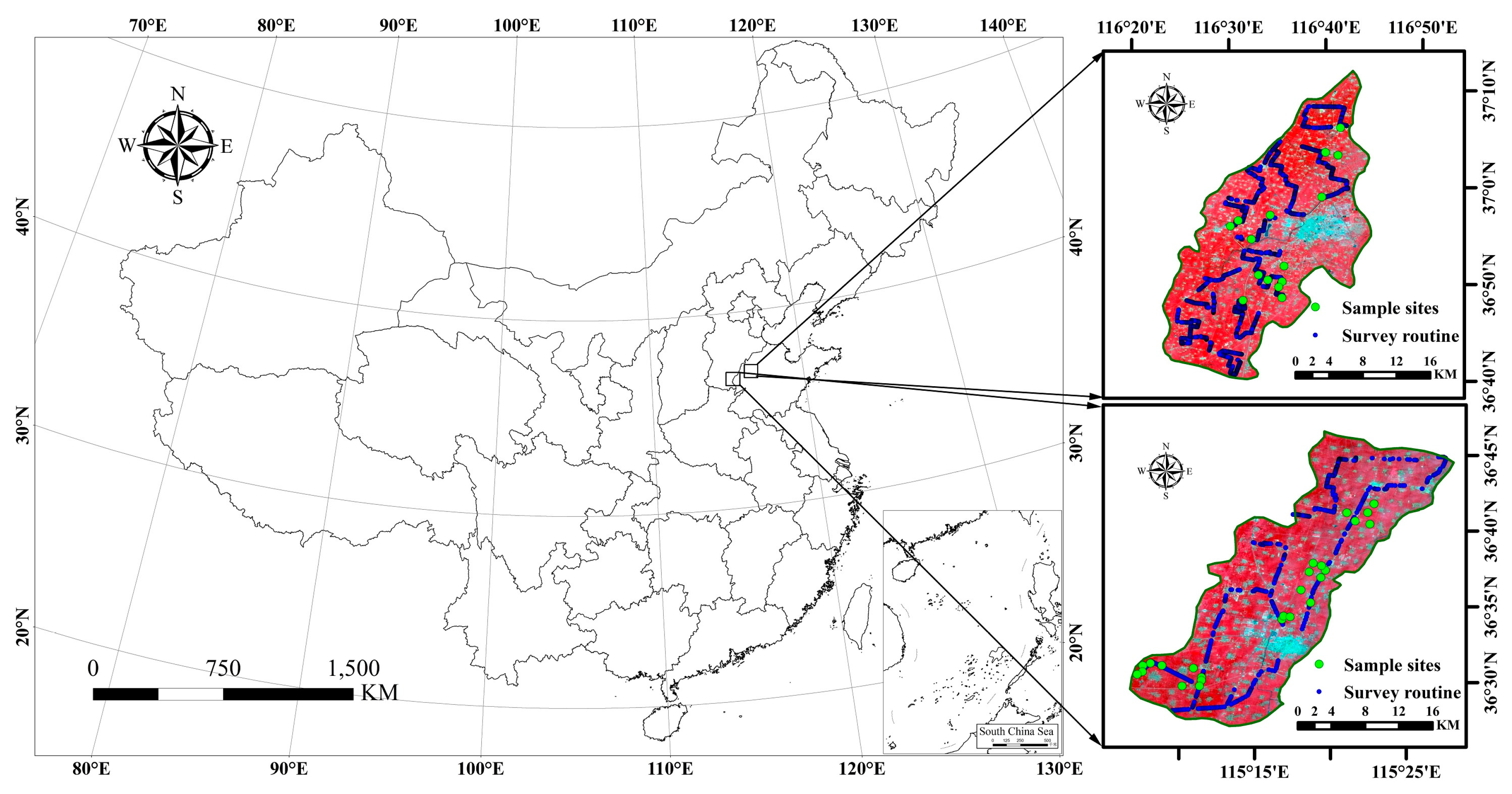
2.1. Study Area
2.2. Data Sources
2.2.1. Field Measured Data
2.2.2. Satellite Data
2.2.3. Meteorological Data
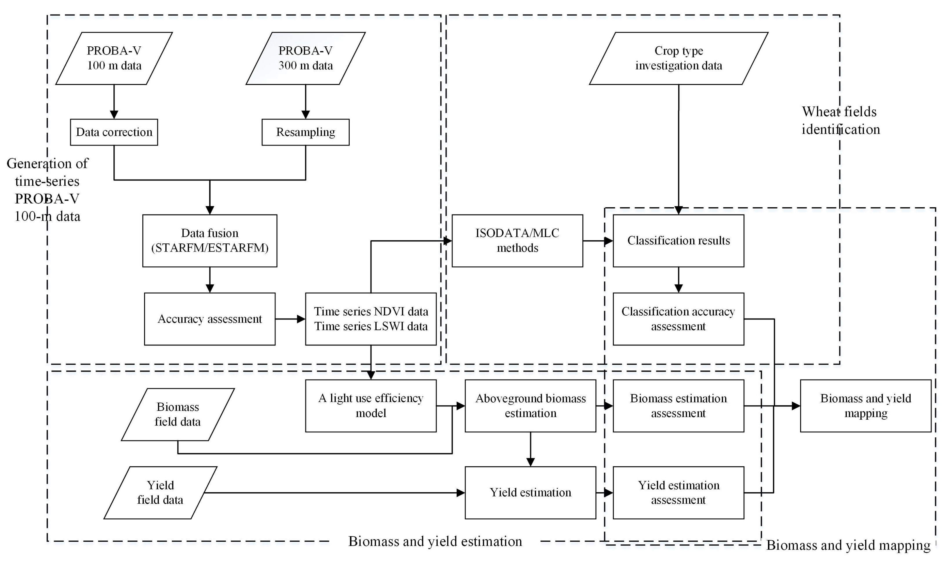
3. Methods
3.1. Daily 100-m Reflectance Dataset Generation
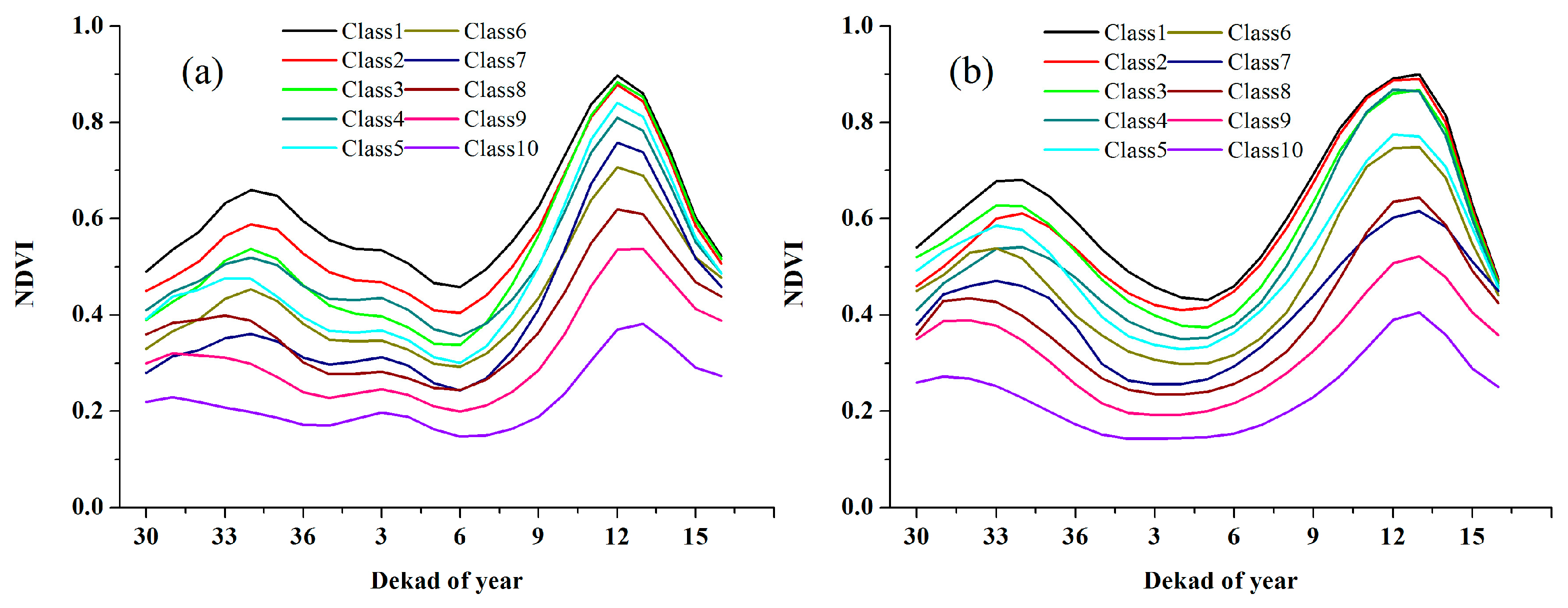
3.2. Crop Identification Based on Time-Series NDVI Clustering
3.3. Algorithms for Biomass and Yield Estimation
3.4. Results Evaluation Strategy
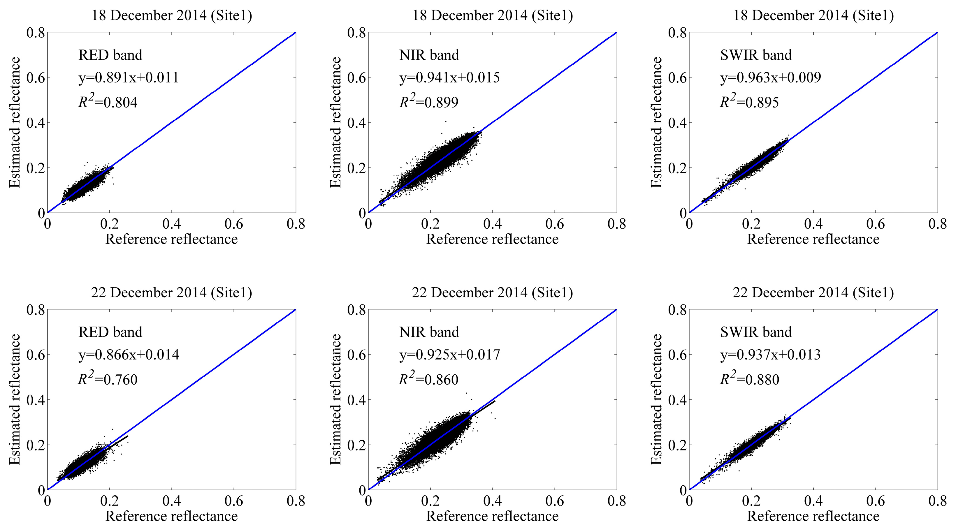
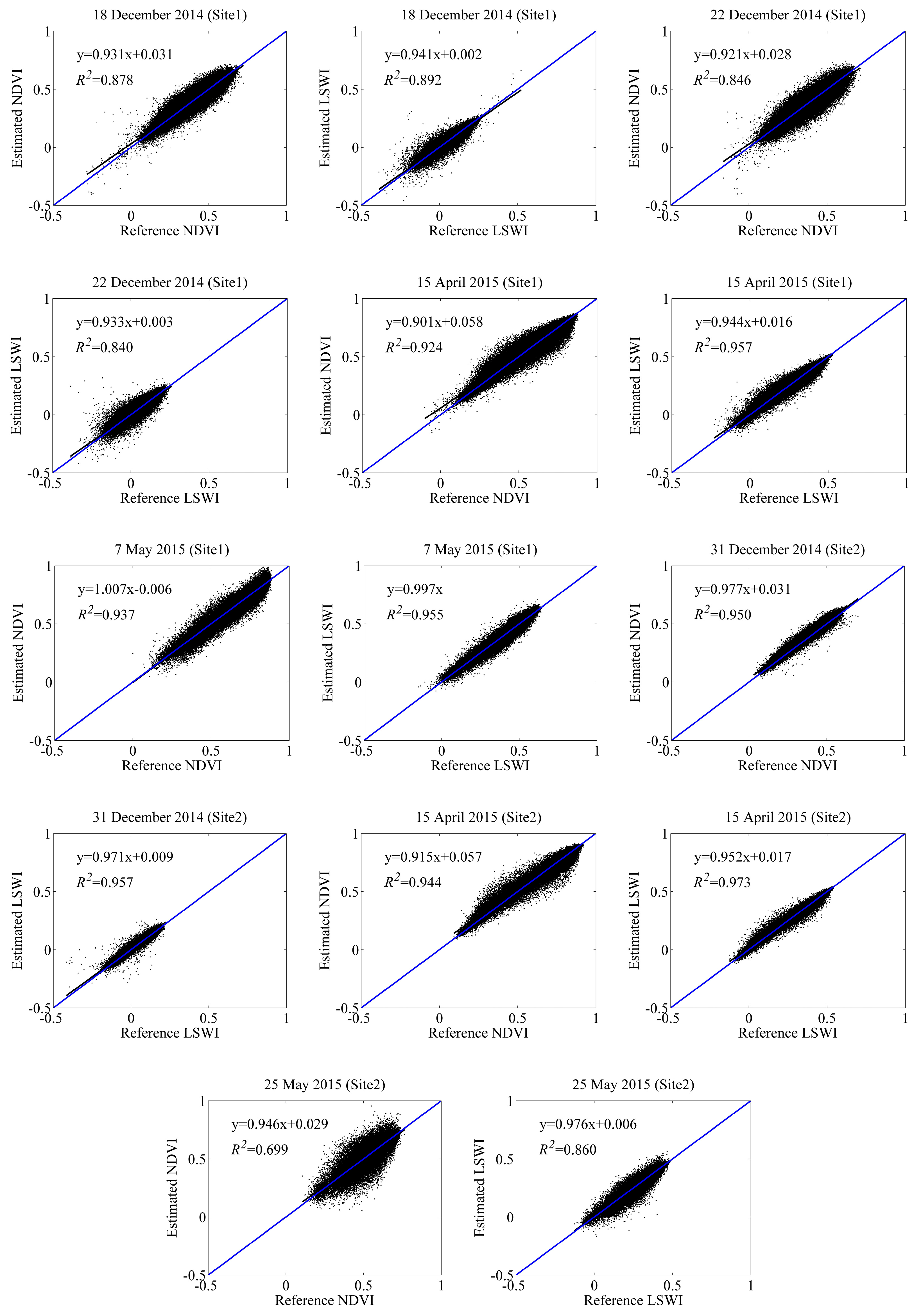
3.4.1. Evaluation of the Data Fusion Result
3.4.2. Assessment of Biomass and Yield Estimation
4. Results
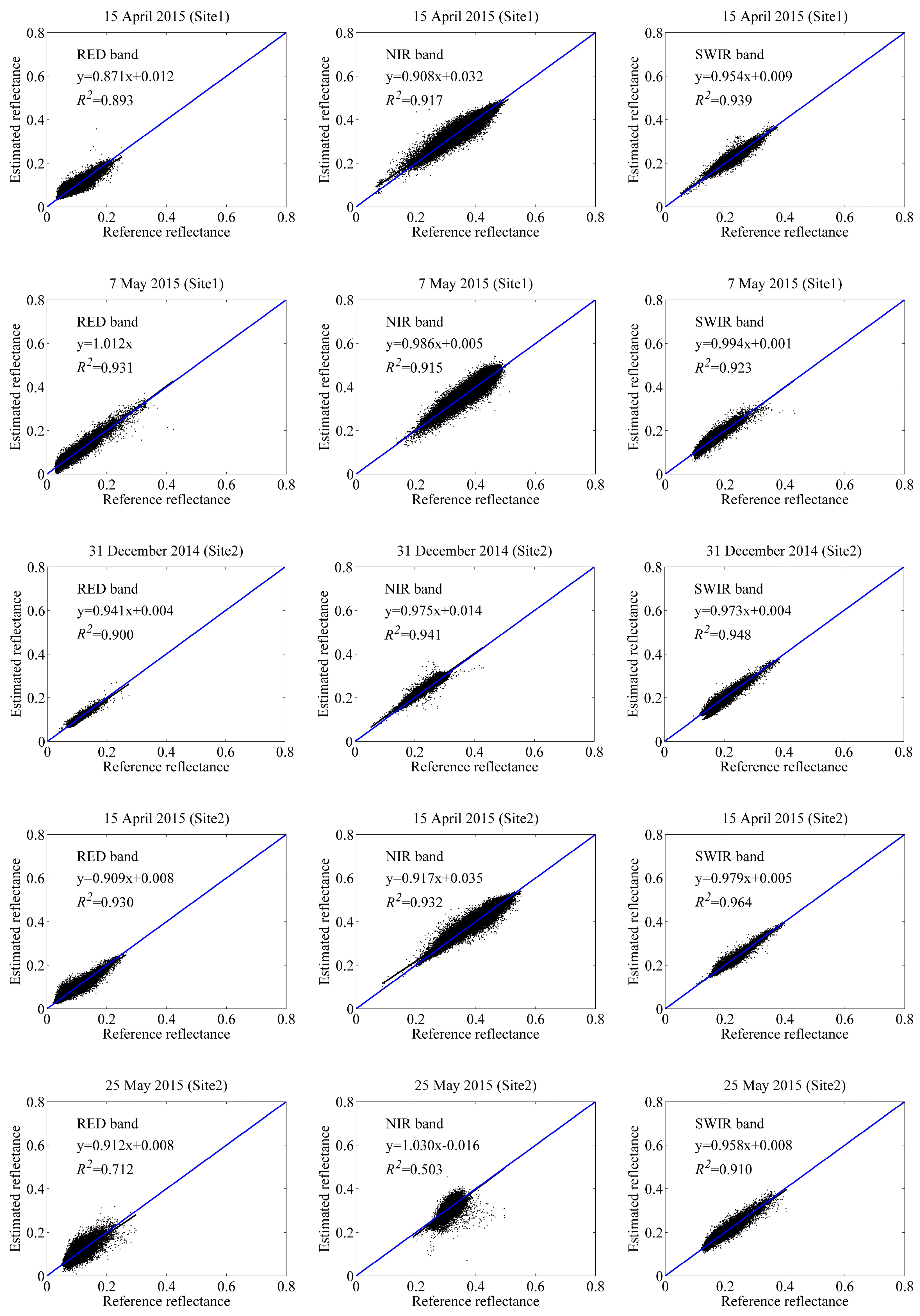
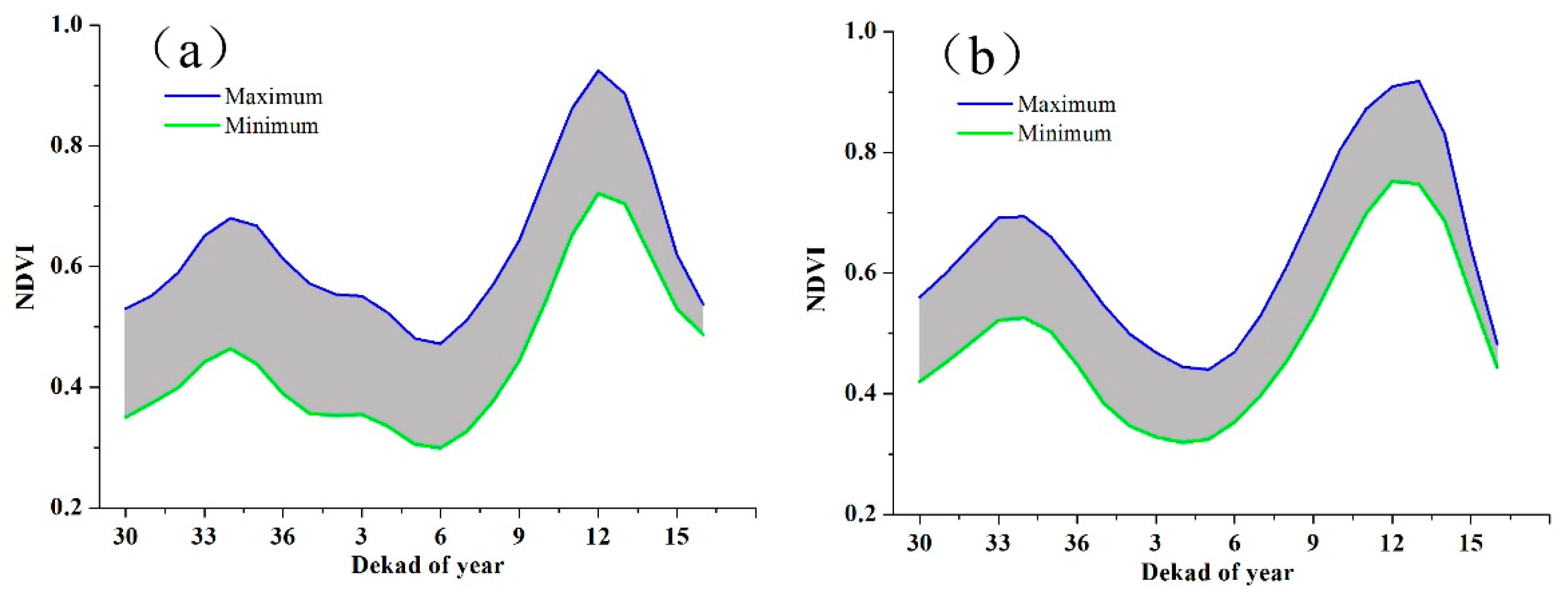
4.1. The ESTARFM Prediction Results
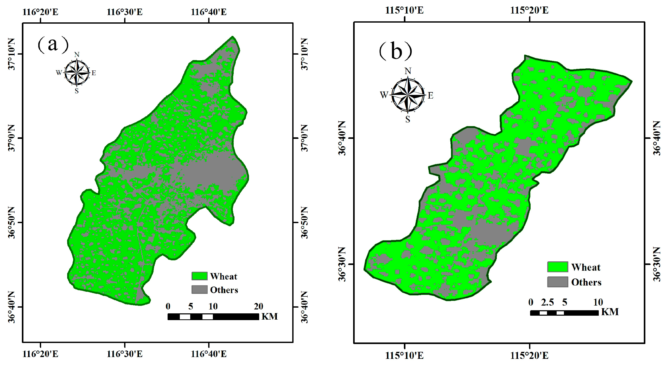
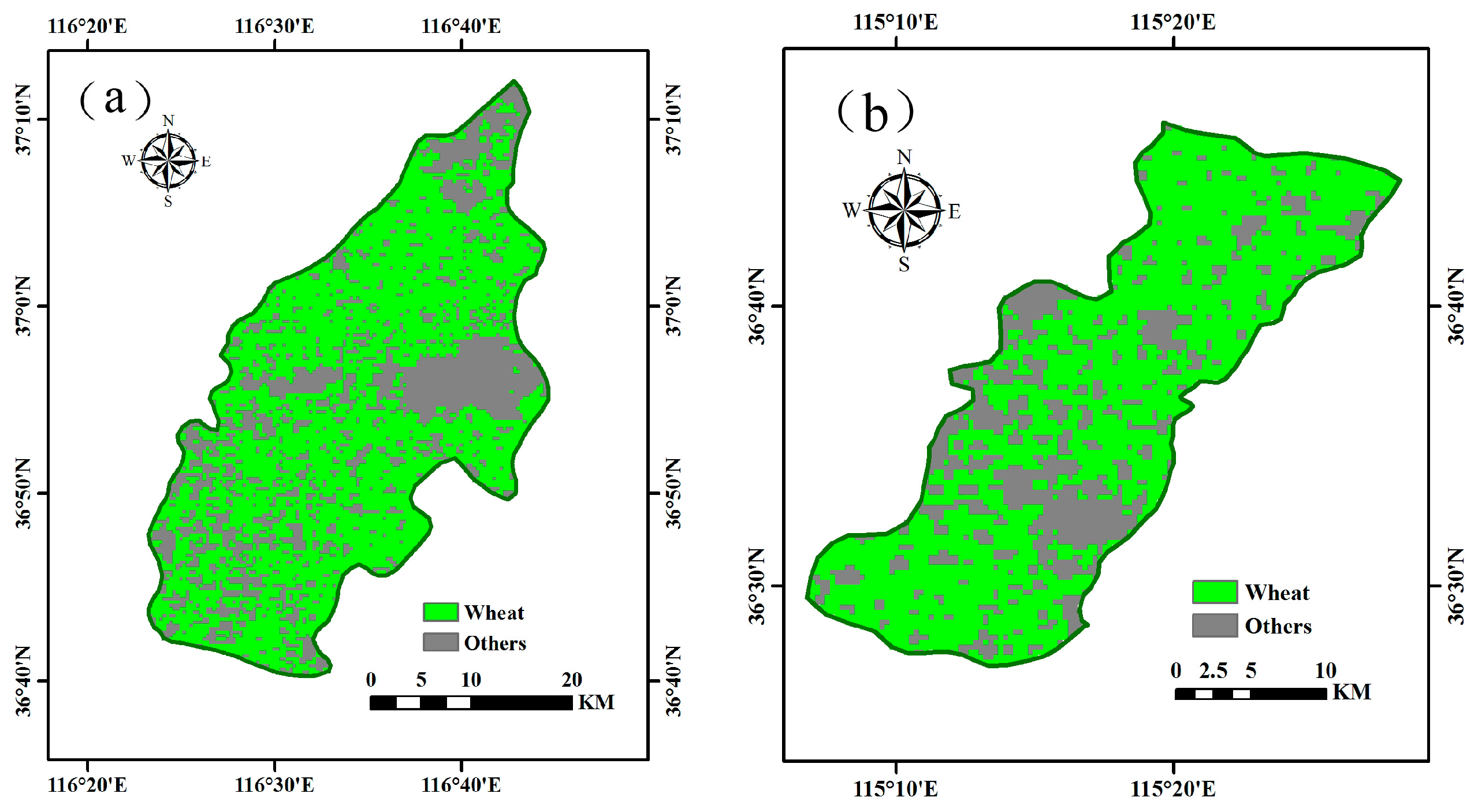
4.2. Generation of Winter Wheat Maps
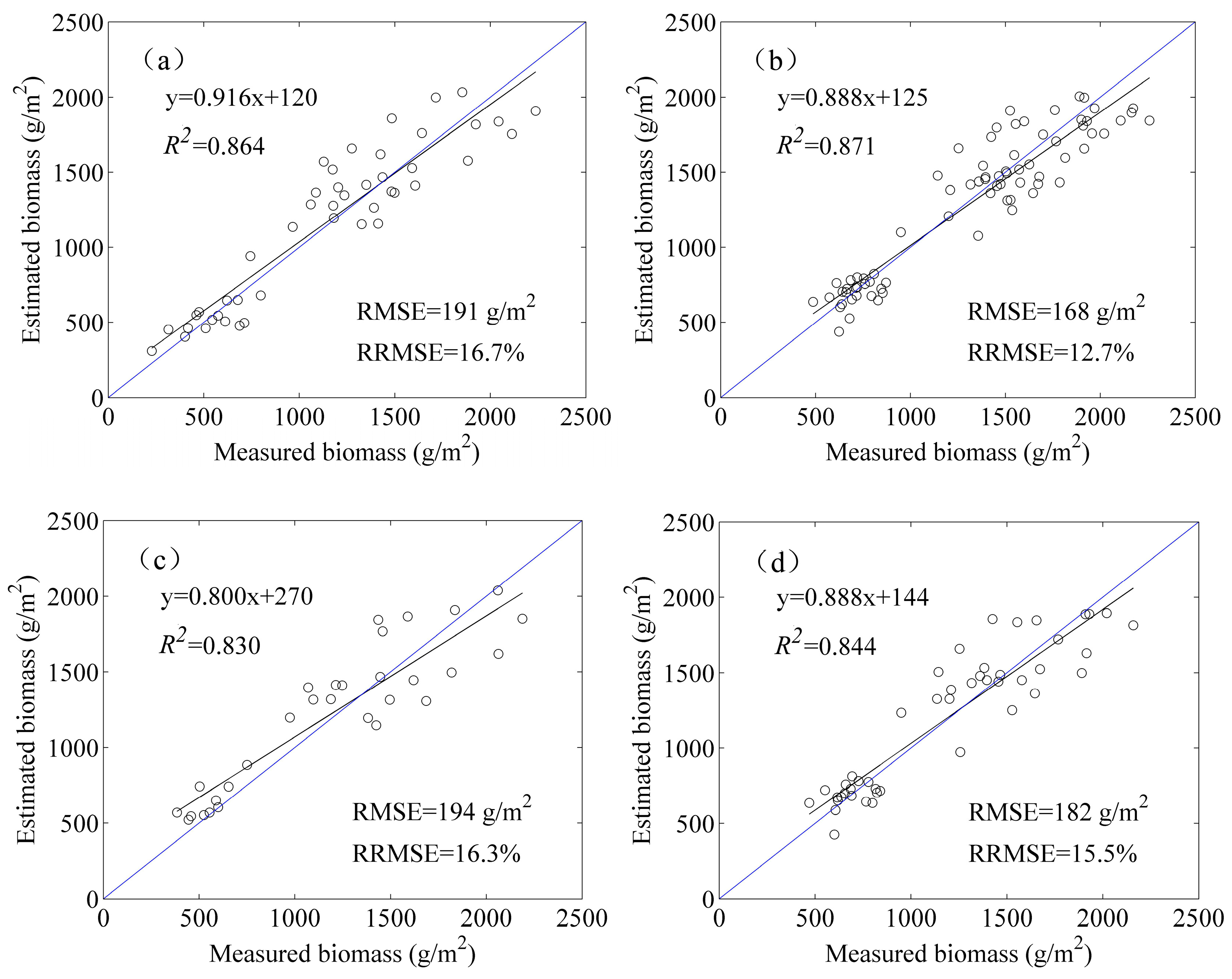
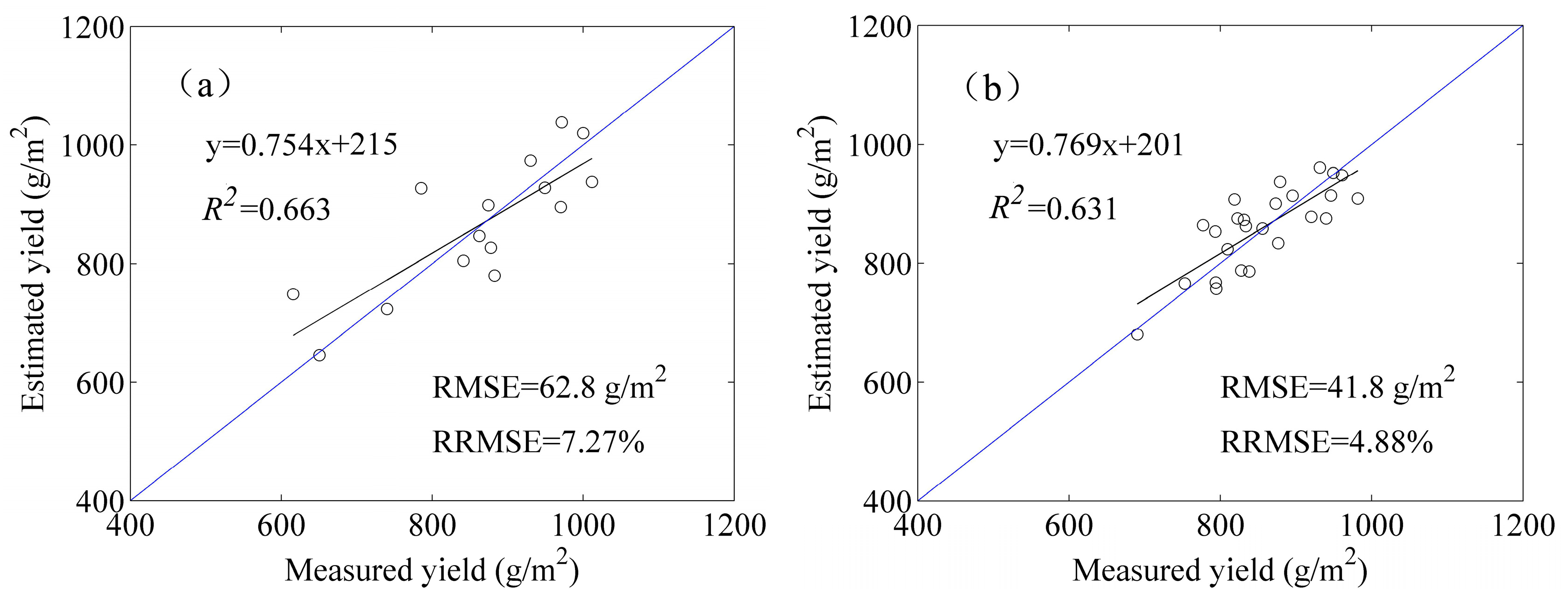
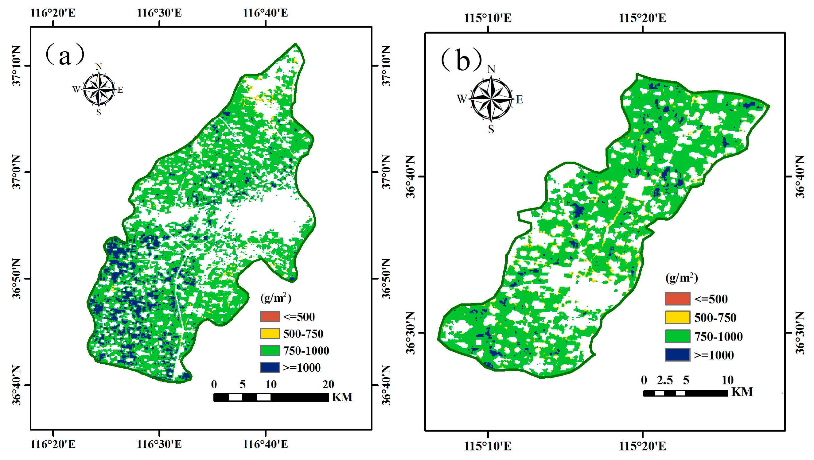
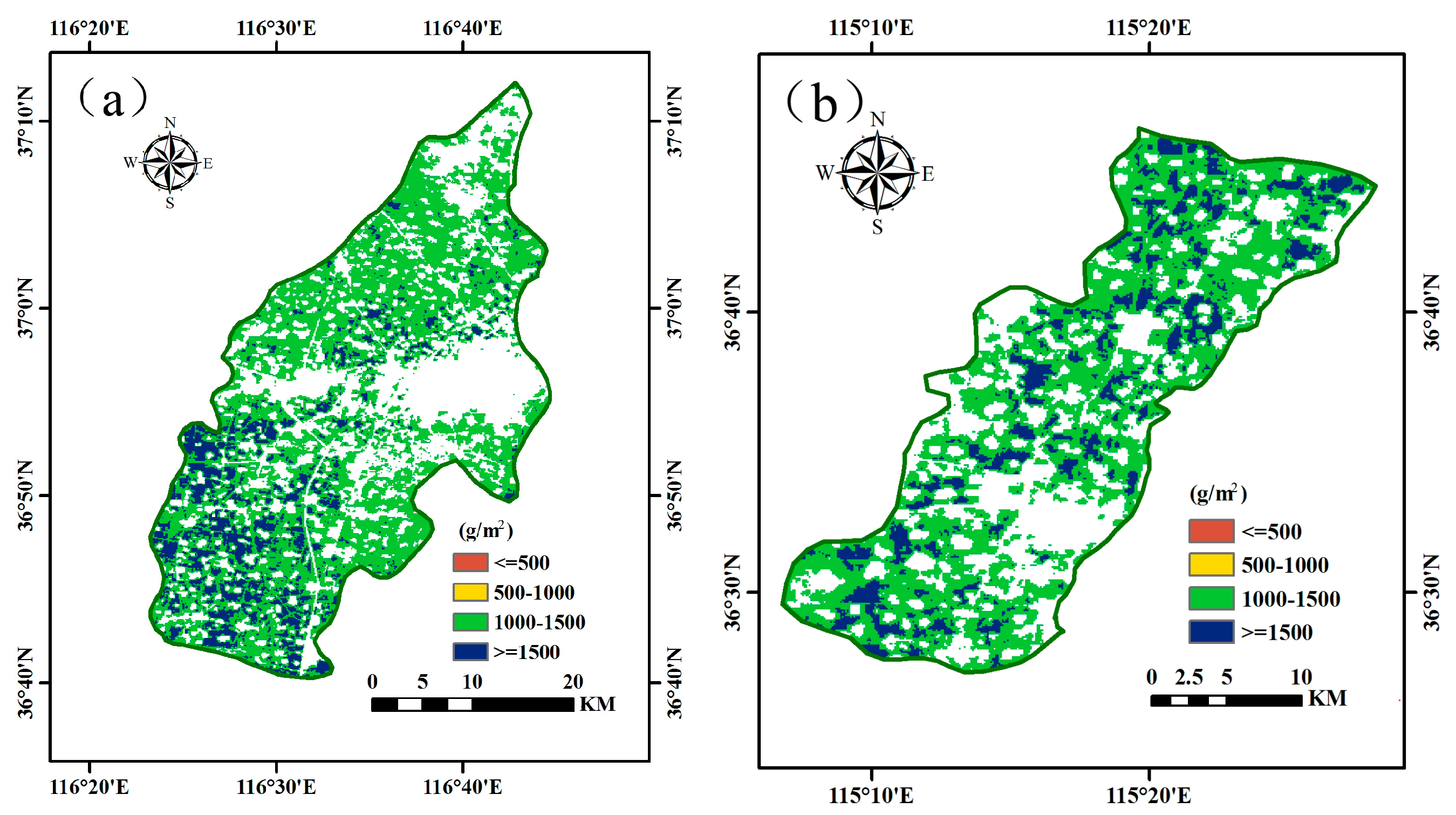
4.3. Mapping the Biomass and Yield
5. Discussion
5.1. Data Fusion Methods
5.2. Mixed Pixels
5.3. LUE
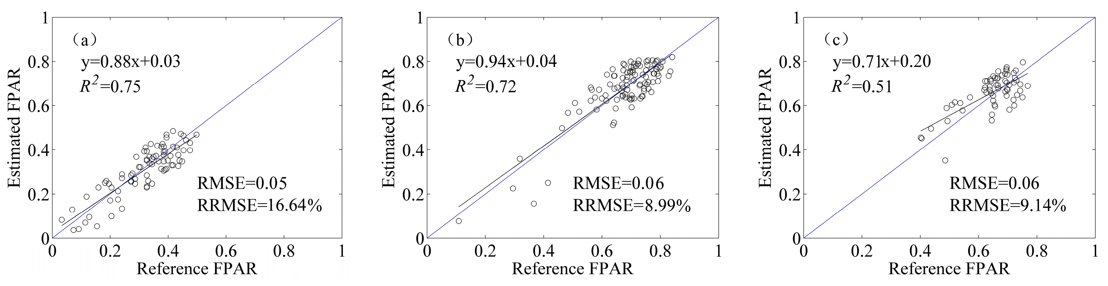
5.4. FPAR
5.5. Meteorological Data
6. Conclusions
Acknowledgments
Author Contributions
Conflicts of Interest
References
- Atzberger, C. Advances in remote sensing of agriculture: Context description, existing operational monitoring systems and major information needs. Remote Sens. 2013, 5, 949–981. [Google Scholar] [CrossRef]
- Godfray, H.C.J.; Beddington, J.R.; Crute, I.R.; Haddad, L.; Lawrence, D.; Muir, J.F.; Pretty, J.; Robinson, S.; Thomas, S.M.; Toulmin, C. Food security: The challenge of feeding 9 billion people. Science 2010, 327, 812–818. [Google Scholar] [CrossRef] [PubMed]
- FAO; IFAD; WFP. The State of Food Insecurity in the World 2014: Strengthening the Enabling Environment for Food Security and Nutrition; Food and Agriculture Organization of the United Nations (FAO): Rome, Italy, 2014; pp. 8–12. [Google Scholar]
- FAO Regional Office for Asia and the Pacific. FAO statistical Yearbook 2014, Asia and the Pacific, Food and Agriculture; FAO Regional Office for Asia and the Pacific: Bangkok, Thailand, 2014; pp. 71–99. [Google Scholar]
- Bao, Y.; Gao, W.; Gao, Z. Estimation of winter wheat biomass based on remote sensing data at various spatial and spectral resolutions. Front. Earth Sci. China 2009, 3, 118–128. [Google Scholar] [CrossRef]
- Jin, X.; Yang, G.; Xu, X.; Yang, H.; Feng, H.; Li, Z.; Shen, J.; Lan, Y.; Zhao, C. Combined multi-temporal optical and radar parameters for estimating LAI and biomass in winter wheat using HJ and RADARSAT-2 data. Remote Sens. 2015, 7, 13251–13272. [Google Scholar] [CrossRef]
- Kross, A.; McNairn, H.; Lapen, D.; Sunohara, M.; Champagne, C. Assessment of RapidEye vegetation indices for estimation of leaf area index and biomass in corn and soybean crops. Int. J. Appl. Earth Obs. Geoinf. 2015, 34, 235–248. [Google Scholar] [CrossRef]
- Du, X.; Li, Q.; Dong, T.; Jia, K. Winter wheat biomass estimation using high temporal and spatial resolution satellite data combined with a light use efficiency model. Geocarto Int. 2014, 30, 258–269. [Google Scholar] [CrossRef]
- Xin, Q.; Gong, P.; Yu, C.; Yu, L.; Broich, M.; Suyker, A.; Myneni, R. A production efficiency model-based method for satellite estimates of corn and soybean yields in the Midwestern US. Remote Sens. 2013, 5, 5926–5943. [Google Scholar] [CrossRef]
- Monteith, J. Climate and efficiency of crop production in Britain. Philos. Trans. R. Soc. Lond. B Biol. Sci. 1977, 281, 277–294. [Google Scholar] [CrossRef]
- Field, C.B.; Randerson, J.T.; MalmstrOm, C.M. Global net primary production: Combining ecology and remote sensing. Remote Sens. Environ. 1995, 51, 74–88. [Google Scholar] [CrossRef]
- Monteith, J. Solar radiation and productivity in tropical ecosystems. J. Appl. Ecol. 1972, 9, 747–766. [Google Scholar] [CrossRef]
- Fensholt, R.; Rasmussen, K.; Nielsen, T.T.; Mbow, C. Evaluation of earth observation based long term vegetation trends—Intercomparing NDVI time series trend analysis consistency of sahel from AVHRR GIMMS, TERRA MODIS and SPOT VGT data. Remote Sens. Environ. 2009, 113, 1886–1898. [Google Scholar] [CrossRef]
- Maisongrande, P.; Duchemin, B.; Dedieu, G. Vegetation/spot: An operational mission for the earth monitoring; presentation of new standard products. Int. J. Remote Sens. 2004, 25, 9–14. [Google Scholar] [CrossRef]
- Wolters, E.; Dierckx, W.; Swinnen, E. PROBA-V Products User Manual v1.3; European Space Agency (ESA): Paris, France, 2015; p. 10. [Google Scholar]
- Roumenina, E.; Atzberger, C.; Vassilev, V.; Dimitrov, P.; Kamenova, I.; Banov, M.; Filchev, L.; Jelev, G. Single- and multi-date crop identification using PROBA-V 100 and 300 m S1 products on Zlatia test site, Bulgaria. Remote Sens. 2015, 7, 13843–13862. [Google Scholar] [CrossRef]
- Marie-Julie, L.; François, W.; Defourny, P. Cropland mapping over Sahelian and Sudanian agrosystems: A knowledge-based approach using PROBA-V time series at 100-m. Remote Sens. 2016, 8, 232–254. [Google Scholar]
- Michele, M.; Dominique, F.; Riad, B.; Mustapha, D.; Myriam, H.; Ismael, H.; Josh, H.; Mouanis, L.; Raul, L.-L.; Hamid, M.; et al. Evaluating NDVI data continuity between SPOT-VEGETATION and PROBA-V missions for operational yield forecasting in North African countries. IEEE Trans. Geosci. Remote Sens. 2016, 54, 795–804. [Google Scholar]
- Walker, J.J.; de Beurs, K.M.; Wynne, R.H.; Gao, F. Evaluation of Landsat and MODIS data fusion products for analysis of dryland forest phenology. Remote Sens. Environ. 2012, 117, 381–393. [Google Scholar] [CrossRef]
- Hansen, M.C.; Roy, D.P.; Lindquist, E.; Adusei, B.; Justice, C.O.; Altstatt, A. A method for integrating MODIS and Landsat data for systematic monitoring of forest cover and change in the Congo Basin. Remote Sens. Environ. 2008, 112, 2495–2513. [Google Scholar] [CrossRef]
- Jia, K.; Liang, S.; Wei, X.; Yao, Y.; Su, Y.; Jiang, B.; Wang, X. Land cover classification of Landsat data with phenological features extracted from time series MODIS NDVI data. Remote Sens. 2014, 6, 11518–11532. [Google Scholar] [CrossRef]
- Gao, F.; Masek, J.; Schwaller, M.; Hall, F. On the blending of the Landsat and MODIS surface reflectance: Predicting daily Landsat surface reflectance. IEEE Trans. Geosci. Remote Sens. 2006, 44, 2207–2218. [Google Scholar]
- Meng, J.; Du, X.; Wu, B. Generation of high spatial and temporal resolution NDVI and its application in crop biomass estimation. Int. J. Digit. Earth 2013, 6, 203–218. [Google Scholar] [CrossRef]
- Zhu, X.; Chen, J.; Gao, F.; Chen, X.; Masek, J.G. An enhanced spatial and temporal adaptive reflectance fusion model for complex heterogeneous regions. Remote Sens. Environ. 2010, 114, 2610–2623. [Google Scholar] [CrossRef]
- Dierckx, W.; Sterckx, S.; Benhadj, I.; Livens, S.; Duhoux, G.; Van Achteren, T.; Francois, M.; Mellab, K.; Saint, G. PROBA-V mission for global vegetation monitoring: Standard products and image quality. Int. J. Remote Sens. 2014, 35, 2589–2614. [Google Scholar] [CrossRef]
- Sterckx, S.; Benhadj, I.; Duhoux, G.; Livens, S.; Dierckx, W.; Goor, E.; Adriaensen, S.; Heyns, W.; Van Hoof, K.; Strackx, G.; et al. The PROBA-V mission: Image processing and calibration. Int. J. Remote Sens. 2014, 35, 2565–2588. [Google Scholar] [CrossRef]
- Francois, M.; Santandrea, S.; Mellab, K.; Vrancken, D.; Versluys, J. The PROBA-V mission: The space segment. Int. J. Remote Sens. 2014, 35, 2548–2564. [Google Scholar] [CrossRef]
- The VITO. Product Distribution Portal (PDF). Available online: http://www.vito-eodata.be/PDF/portal/Application.html#Home (accessed on 16 April 2016).
- SPIRITS. Institute for Environment and Sustainability. Available online: http://spirits.jrc.ec.europa.eu/ (accessed on 20 March 2016).
- Eerens, H.; Haesen, D.; Rembold, F.; Urbano, F.; Tote, C.; Bydekerke, L. Image time series processing for agriculture monitoring. Environ. Model. Softw. 2014, 53, 154–162. [Google Scholar] [CrossRef]
- Rembold, F.; Meroni, M.; Urbano, F.; Royer, A.; Atzberger, C.; Lemoine, G.; Eerens, H.; Haesen, D. Remote sensing time series analysis for crop monitoring with the SPIRITS software: New functionalities and use examples. Front. Environ. Sci. 2015, 3, 46. [Google Scholar] [CrossRef]
- China Meteorological Data Sharing Service System. Available online: http://data.cma.cn (accessed on 11 January 2016).
- Richard, G.A.; Luis, S.P.; Dirk, R.; Martin, S. Crop Evapotranspiration: Guidelines for Computing Crop Water Requirements; Irrigation and drainage paper; Food and Agriculture Organization of the United Nations (FAO): Rome, Italy, 1998; pp. 89–102. [Google Scholar]
- Liu, H.; Weng, Q. Enhancing temporal resolution of satellite imagery for public health studies: A case study of West Nile Virus outbreak in Los Angeles in 2007. Remote Sens. Environ. 2012, 117, 57–71. [Google Scholar] [CrossRef]
- Zhang, F.; Zhu, X.; Liu, D. Blending MODIS and Landsat images for urban flood mapping. Int. J. Remote Sens. 2014, 35, 3237–3253. [Google Scholar] [CrossRef]
- Knauer, K.; Gessner, U.; Fensholt, R.; Kuenzer, C. An ESTARFM fusion framework for the generation of large-scale time series in cloud-prone and heterogeneous landscapes. Remote Sens. 2016, 8, 425. [Google Scholar] [CrossRef]
- Huang, C.; Chen, Y.; Zhang, S.; Li, L.; Shi, K.; Liu, R. Surface water mapping from Suomi NPP-VIIRS imagery at 30 m resolution via blending with Landsat data. Remote Sens. 2016, 8, 631. [Google Scholar] [CrossRef]
- Liu, X.; Bo, Y.; Zhang, J.; He, Y. Classification of C3 and C4 vegetation types using MODIS and ETM+ blended high spatio-temporal resolution data. Remote Sens. 2015, 7, 15244–15268. [Google Scholar] [CrossRef]
- Xiao, X.; Hollinger, D.; Aber, J.; Goltz, M.; Davidson, E.A.; Zhang, Q.; Moore, B. Satellite-based modeling of gross primary production in an evergreen needleleaf forest. Remote Sens. Environ. 2004, 89, 519–534. [Google Scholar] [CrossRef]
- Xiao, X.; Zhang, Q.; Saleska, S.; Hutyra, L.; De Camargo, P.; Wofsy, S.; Frolking, S.; Boles, S.; Keller, M.; Moore, B. Satellite-based modeling of gross primary production in a seasonally moist tropical evergreen forest. Remote Sens. Environ. 2005, 94, 105–122. [Google Scholar] [CrossRef]
- Rouse, J.W.; Haas, R.H. Monitoring vegetation systems in the great plains with erts. In Proceedings of the Third Earth Resources Technology Satellite Symposium, Washington, DC, USA, 10–14 December 1973; pp. 309–317.
- Chen, J.; Jönsson, P.; Tamura, M.; Gu, Z.; Matsushita, B.; Eklundh, L. A simple method for reconstructing a high-quality NDVI time-series data set based on the Savitzky–Golay filter. Remote Sens. Environ. 2004, 91, 332–344. [Google Scholar] [CrossRef]
- Savitzky, A.; Golay, M.J.E. Smoothing and differentiation of data by simplified least squares procedures. Anal. Chem. 1964, 36, 1627–1639. [Google Scholar] [CrossRef]
- Simonneaux, V.; Duchemin, B.; Helson, D.; Er-Raki, S.; Olioso, A.; Chehbouni, A.G. The use of high-resolution image time series for crop classification and evapotranspiration estimate over an irrigated area in central Morocco. Int. J. Remote Sens. 2008, 29, 95–116. [Google Scholar] [CrossRef]
- Sellers, P.J.; Randall, D.A.; Collatz, G.J.; Berry, J.A.; Field, C.B.; Dazlich, D.A.; Zhang, C.; Collelo, G.D.; Bounoua, L. A revised Land Surface parameterization (SiB2) for atmospheric GCMs. Part I: Model Formulation. J. Clim. 1996, 9, 676–705. [Google Scholar] [CrossRef]
- Lobell, D.B.; Asnera, G.P.; Ortiz-Monasteriob, J.I.; Benning, T.L. Remote sensing of regional crop production in the Yaqui Valley, Mexico: Estimates and uncertainties. Agric. Ecosyst. Environ. 2003, 94, 205–220. [Google Scholar] [CrossRef]
- Kemanian, A.R.; Stöckle, C.O.; Huggins, D.R.; Viega, L.M. A simple method to estimate harvest index in grain crops. Field Crops Res. 2007, 103, 208–216. [Google Scholar] [CrossRef]
- Shao, J. Linear model selection by cross-validation. J. Am. Stat. Assoc. 1993, 88, 486–494. [Google Scholar] [CrossRef]
- Tewes, A.; Thonfeld, F.; Schmidt, M.; Oomen, R.; Zhu, X.; Dubovyk, O.; Menz, G.; Schellberg, J. Using RapidEye and MODIS data fusion to monitor vegetation dynamics in semi-arid rangelands in South Africa. Remote Sens. 2015, 7, 6510–6534. [Google Scholar] [CrossRef]
- Battude, M.; Al Bitar, A.; Morin, D.; Cros, J.; Huc, M.; Marais Sicre, C.; Le Dantec, V.; Demarez, V. Estimating maize biomass and yield over large areas using high spatial and temporal resolution sentinel-2 like remote sensing data. Remote Sens. Environ. 2016, 184, 668–681. [Google Scholar] [CrossRef]
- Hao, P.; Wang, L.; Niu, Z.; Aablikim, A.; Huang, N.; Xu, S.; Chen, F. The potential of time series merged from Landsat-5 TM and HJ-1 CCD for crop classification: A case study for bole and manas counties in Xinjiang, China. Remote Sens. 2014, 6, 7610–7631. [Google Scholar] [CrossRef]
- Siachalou, S.; Mallinis, G.; Tsakiri-Strati, M. A hidden Markov models approach for crop classification: Linking crop phenology to time series of multi-sensor remote sensing data. Remote Sens. 2015, 7, 3633–3650. [Google Scholar] [CrossRef]
- Hadria, R.; Duchemin, B.; Jarlan, L.; Dedieu, G.; Baup, F.; Khabba, S.; Olioso, A.; Le Toan, T. Potentiality of optical and radar satellite data at high spatio-temporal resolutions for the monitoring of irrigated wheat crops in Morocco. Int. J. Appl. Earth Obs. Geoinf. 2010, 12, S32–S37. [Google Scholar] [CrossRef]
- Dong, T.; Liu, J.; Qian, B.; Zhao, T.; Jing, Q.; Geng, X.; Wang, J.; Huffman, T.; Shang, J. Estimating winter wheat biomass by assimilating leaf area index derived from fusion of Landsat-8 and MODIS data. Int. J. Appl. Earth Obs. Geoinf. 2016, 49, 63–74. [Google Scholar] [CrossRef]
- Immitzer, M.; Vuolo, F.; Atzberger, C. First experience with Sentinel-2 data for crop and tree species classifications in central Europe. Remote Sens. 2016, 8, 166. [Google Scholar] [CrossRef]
- Drusch, M.; Del Bello, U.; Carlier, S.; Colin, O.; Fernandez, V.; Gascon, F.; Hoersch, B.; Isola, C.; Laberinti, P.; Martimort, P.; et al. Sentinel-2: ESA’s optical high-resolution mission for GMES operational services. Remote Sens. Environ. 2012, 120, 25–36. [Google Scholar] [CrossRef]
- Stephanie, D.; Pablo, J.Z.-T.; Laurent, T.; Miguel, Á.J.B.; Diego, S.I.; Ben, S. Unmixing-based fusion of hyperspatial and hyperspectral airborne imagery for early detection of vegetation stress. IEEE J. Sel. Top. Appl. Earth Obs. Remote Sens. 2014, 7, 2571–2582. [Google Scholar]
- Li, Q.; Chen, Y.; Liu, M.; Zhou, X.; Yu, S.; Dong, B. Effects of irrigation and planting patterns on radiation use efficiency and yield of winter wheat in North China. Agric. Water Manag. 2008, 95, 469–476. [Google Scholar] [CrossRef]
- Rosati, A.; Dejong, T. Estimating photosynthetic radiation use efficiency using incident light and photosynthesis of individual leaves. Ann. Bot. 2003, 91, 869–877. [Google Scholar] [CrossRef] [PubMed]
- Sinclair, T.R.; Muchow, R.C. Radiation use efficiency. Adv. Agron. 1999, 65, 215–265. [Google Scholar]
- O’Connell, M.; O’Leary, G.; Whitfield, D.; Connor, D. Interception of photosynthetically active radiation and radiation-use efficiency of wheat, field pea and mustard in a semi-arid environment. Field Crops Res. 2004, 85, 111–124. [Google Scholar] [CrossRef]
- Kiniry, J.; Jones, C.; Otoole, J.; Blanchet, R.; Cabelguenne, M.; Spanel, D. Radiation-use efficiency in biomass accumulation prior to grain-filling for 5 grain-crop species. Field Crops Res. 1989, 20, 51–64. [Google Scholar] [CrossRef]
- Duchemin, B.; Maisongrande, P.; Boulet, G.; Benhadj, I. A simple algorithm for yield estimates: Evaluation for semi-arid irrigated winter wheat monitored with green leaf area index. Environ. Model. Softw. 2008, 23, 876–892. [Google Scholar] [CrossRef]
- Garcia, R.; Kanemasu, E.; Blad, B.; Bauer, A.; Hatfield, J.; Major, D.; Reginato, R.; Hubbard, K. Interception and use efficiency of light in winter-wheat under different nitrogen regimes. Agric. For. Meteorol. 1988, 44, 175–186. [Google Scholar] [CrossRef]
- Tao, F.; Yokozawa, M.; Zhang, Z.; Xu, Y.; Hayashi, Y. Remote sensing of crop production in China by production efficiency models: Models comparisons, estimates and uncertainties. Ecol. Model. 2005, 183, 385–396. [Google Scholar] [CrossRef]
- Ruimy, A.; Saugie, B.; Dedieu, G. Methodology for the estimation of terrestrial net primary production from remotely sensed data. J. Geophys. Res. 1994, 99, 5263–5283. [Google Scholar] [CrossRef]
- Zhang, Y.; Tang, Q.; Zou, Y.; Li, D.; Qin, J.; Yang, S.; Chen, L.; Xia, B.; Peng, S. Yield potential and radiation use efficiency of “super” hybrid rice grown under subtropical conditions. Field Crops Res. 2009, 114, 91–98. [Google Scholar] [CrossRef]
- Peng, D.; Huang, J.; Li, C.; Liu, L.; Huang, W.; Wang, F.; Yang, X. Modelling paddy rice yield using MODIS data. Agric. For. Meteorol. 2014, 184, 107–116. [Google Scholar] [CrossRef]
- Roumenina, E.; Kazandjiev, V.; Dimitrov, P.; Filchev, L.; Vassilev, V.; Jelev, G.; Georgieva, V.; Lukarski, H. Validation of LAI and assessment of winter wheat status using spectral data and vegetation indices from SPOT VEGETATION and simulated PROBA-V images. Int. J. Remote Sens. 2013, 34, 2888–2904. [Google Scholar] [CrossRef]
- Cheng, Y.-B.; Zhang, Q.; Lyapustin, A.I.; Wang, Y.; Middleton, E.M. Impacts of light use efficiency and FPAR parameterization on gross primary production modeling. Agric. For. Meteorol. 2014, 189–190, 187–197. [Google Scholar] [CrossRef]
- The European System for Monitoring the Earth. Available online: http://www.copernicus.eu/ (accessed on 11 April 2016).
- Dong, T.; Meng, J.; Shang, J.; Liu, J.; Wu, B.; Huffman, T. Modified vegetation indices for estimating crop fraction of absorbed photosynthetically active radiation. Int. J. Remote Sens. 2015, 36, 3097–3113. [Google Scholar] [CrossRef]
- Peng, Y.; Gitelson, A.A. Remote estimation of gross primary productivity in soybean and maize based on total crop chlorophyll content. Remote Sens. Environ. 2012, 117, 440–448. [Google Scholar] [CrossRef]
- Viña, A.; Gitelson, A. New developments in the remote estimation of the fraction of absorbed photosynthetically active radiation in crops. Geophys. Res. Lett. 2005, 32. [Google Scholar] [CrossRef]
- McCallum, I.; Wagner, W.; Schmullius, C.; Shvidenko, A.; Obersteiner, M.; Fritz, S.; Nilsson, S. Comparison of four global FPAR datasets over Northern Eurasia for the year 2000. Remote Sens. Environ. 2010, 114, 941–949. [Google Scholar] [CrossRef]
- Thornton, P.; Running, S.; White, M. Generating surfaces of daily meteorological variables over large regions of complex terrain. J. Hydrol. 1997, 190, 214–251. [Google Scholar] [CrossRef]
- Liu, R.; Liang, S.; He, H.; Liu, J.; Zheng, T. Mapping incident photosynthetically active radiation from MODIS data over China. Remote Sens. Environ. 2008, 112, 998–1009. [Google Scholar]


| Study Sites | Crop Type | Sample Date | Growing Stage | Number (N) |
|---|---|---|---|---|
| Site 1 | Winter WHEAT | 16 April 2015 | Booting | 25 |
| 17 May 2015 | Flowering | 25 | ||
| 4 June 2015 | Harvest | 25 | ||
| Site 2 | Winter Wheat | 15 April 2015 | Booting | 15 |
| 17 May 2015 | Flowering | 15 | ||
| 6 June 2015 | Harvest | 15 |
| Crop Types | Site 1 | Site 2 | ||
|---|---|---|---|---|
| Date | Good Pixels Ratio | Date | Good Pixels Ratio | |
| Winter wheat | 2 November 2014 | 100% | 2 November 2014 | 100% |
| 13 December 2014 | 100% | 13 December 2014 | 100% | |
| 18 December 2014 | 100% | 31 December 2014 | 100% | |
| 22 December 2014 | 100% | 9 January 2015 | 100% | |
| 31 December 2014 | 100% | 10 February 2015 | 100% | |
| 19 January 2015 | 99% | 27 March 2015 | 100% | |
| 10 February 2015 | 100% | 10 April 2015 | 100% | |
| 28 March 2015 | 98% | 15 April 2015 | 100% | |
| 10 April 2015 | 99% | 12 May 2015 | 97% | |
| 15 April 2015 | 98% | 25 May 2015 | 99% | |
| 7 May 2015 | 98% | 30 May 2015 | 100% | |
| 16 May 2015 | 100% | - | - | |
| 30 May 2015 | 98% | - | - | |
| Parameter | Description | Value | Unit |
|---|---|---|---|
| the maximum light use efficiency | 2.54 | g·MJ−1 PAR | |
| R | proportion of aboveground productivity | 0.90 | dimensionless |
| HI | the harvest index | 0.45 | dimensionless |
| Indicators | Formula |
|---|---|
| Determination coefficient (R2) | |
| Root mean square errors (RMSE) | |
| Relative RMSE (RRMSE) | |
| Average absolute deviation (AAD) | |
| Average deviation (AD) |
| Sites | Date (100-m) | Date (300-m) | Band | R2 | RMSE | RRMSE | AAD | AD |
|---|---|---|---|---|---|---|---|---|
| Site 1 | 18 December 2014 | 18 December 2014 | RED | 0.804 | 0.0083 | 0.0775 | 0.0650 | 9.5 × 10⁻⁸ |
| NIR | 0.899 | 0.0132 | 0.0536 | 0.0099 | 4.8 × 10⁻⁷ | |||
| SWIR | 0.895 | 0.0062 | 0.0278 | 0.0047 | 3.6 × 10⁻⁷ | |||
| Site 1 | 22 December 2014 | 22 December 2014 | RED | 0.760 | 0.0089 | 0.0838 | 0.0068 | 1.6 × 10⁻⁷ |
| NIR | 0.860 | 0.0145 | 0.0624 | 0.0108 | 3.9 × 10⁻⁷ | |||
| SWIR | 0.880 | 0.0061 | 0.0281 | 0.0046 | 9.6 × 10⁻⁸ | |||
| Site 1 | 15 April 2015 | 15 April 2015 | RED | 0.893 | 0.0109 | 0.1238 | 0.0082 | 1.8 × 10⁻⁷ |
| NIR | 0.917 | 0.0172 | 0.0482 | 0.0130 | 4.7 × 10⁻⁷ | |||
| SWIR | 0.939 | 0.0082 | 0.0412 | 0.0056 | 1.2 × 10⁻⁶ | |||
| Site 1 | 7 May 2015 | 7 May 2015 | RED | 0.931 | 0.0111 | 0.1432 | 0.0082 | 2.0 × 10⁻⁷ |
| NIR | 0.915 | 0.0175 | 0.0464 | 0.0130 | 9.4 × 10⁻⁷ | |||
| SWIR | 0.923 | 0.0086 | 0.0595 | 0.0061 | 3.0 × 10⁻⁷ | |||
| Site 2 | 31 December 2014 | 31 December 2014 | RED | 0.900 | 0.0055 | 0.0522 | 0.0042 | 8.8 × 10⁻⁸ |
| NIR | 0.941 | 0.0094 | 0.0308 | 0.0070 | 1.4 × 10⁻⁷ | |||
| SWIR | 0.948 | 0.0097 | 0.0224 | 0.0067 | 3.5 × 10⁻⁷ | |||
| Site 2 | 15 April 2015 | 15 April 2015 | RED | 0.930 | 0.0112 | 0.1365 | 0.0081 | 5.3 × 10⁻⁸ |
| NIR | 0.932 | 0.0181 | 0.0443 | 0.0134 | 3.9 × 10⁻⁸ | |||
| SWIR | 0.964 | 0.0074 | 0.0356 | 0.0051 | 9.4 × 10⁻⁸ | |||
| Site 2 | 25 May 2015 | 25 May 2015 | RED | 0.712 | 0.0175 | 0.1813 | 0.0122 | 3.1 × 10⁻⁷ |
| NIR | 0.503 | 0.0190 | 0.0592 | 0.0137 | 4.3 × 10⁻⁶ | |||
| SWIR | 0.910 | 0.0115 | 0.0629 | 0.0082 | 3.8 × 10⁻⁷ |
| Sites | Date (100-m) | Date (300-m) | Indices | R2 | RMSE | AAD | AD |
|---|---|---|---|---|---|---|---|
| Site 1 | 18 December 2014 | 18 December 2014 | NDVI | 0.878 | 0.0447 | 0.0344 | 5.9 × 10⁻⁷ |
| LSWI | 0.892 | 0.0285 | 0.0203 | 4.3 × 10⁻⁸ | |||
| Site 1 | 22 December 2014 | 22 December 2014 | NDVI | 0.846 | 0.0379 | 0.0496 | 2.4 × 10⁻⁷ |
| LSWI | 0.840 | 0.0329 | 0.0238 | 5.1 × 10⁻⁸ | |||
| Site 1 | 15 April 2015 | 15 April 2015 | NDVI | 0.924 | 0.0473 | 0.0361 | 6.1 × 10⁻⁷ |
| LSWI | 0.957 | 0.0293 | 0.0215 | 1.7 × 10⁻⁷ | |||
| Site 1 | 7 May 2015 | 7 May 2015 | NDVI | 0.937 | 0.0423 | 0.0316 | 1.6 × 10⁻⁶ |
| LSWI | 0.955 | 0.0281 | 0.0204 | 5.7 × 10⁻⁷ | |||
| Site 2 | 31 December 2014 | 31 December 2014 | NDVI | 0.950 | 0.0274 | 0.0270 | 3.5 × 10⁻⁷ |
| LSWI | 0.957 | 0.0213 | 0.0156 | 2.9 × 10⁻⁸ | |||
| Site 2 | 15 April 2015 | 15 April 2015 | NDVI | 0.944 | 0.0453 | 0.0335 | 1.1 × 10⁻⁶ |
| LSWI | 0.973 | 0.0256 | 0.0181 | 2.5 × 10⁻⁷ | |||
| Site 2 | 25 May 2015 | 25 May 2015 | NDVI | 0.699 | 0.0703 | 0.0509 | 3.7 × 10⁻⁷ |
| LSWI | 0.860 | 0.0407 | 0.0298 | 2.0 × 10⁻⁸ |
| Class | 100-m | 300-m | ||
|---|---|---|---|---|
| Producer’s Accuracy | User’s Accuracy | Producer’s Accuracy | User’s Accuracy | |
| Wheat | 86.96% | 81.63% | 72.83% | 65.05% |
| Others | 82.69% | 87.76% | 65.38% | 73.91% |
| Overall Accuracy: 84.69%; Kappa: 0.7198 | Overall Accuracy: 68.88%; Kappa: 0.3795 | |||
| Class | 100-m | 300-m | ||
|---|---|---|---|---|
| Producer’s Accuracy | User’s Accuracy | Producer’s Accuracy | User’s Accuracy | |
| Wheat | 80.95% | 73.91% | 69.05% | 63.04% |
| Others | 76.62% | 83.1% | 66.88% | 72.54% |
| Overall Accuracy: 78.57%; Kappa: 0.5708 | Overall Accuracy: 67.86%; Kappa: 0.3562 | |||
© 2016 by the authors; licensee MDPI, Basel, Switzerland. This article is an open access article distributed under the terms and conditions of the Creative Commons Attribution (CC-BY) license (http://creativecommons.org/licenses/by/4.0/).
Share and Cite
Zheng, Y.; Zhang, M.; Zhang, X.; Zeng, H.; Wu, B. Mapping Winter Wheat Biomass and Yield Using Time Series Data Blended from PROBA-V 100- and 300-m S1 Products. Remote Sens. 2016, 8, 824. https://doi.org/10.3390/rs8100824
Zheng Y, Zhang M, Zhang X, Zeng H, Wu B. Mapping Winter Wheat Biomass and Yield Using Time Series Data Blended from PROBA-V 100- and 300-m S1 Products. Remote Sensing. 2016; 8(10):824. https://doi.org/10.3390/rs8100824
Chicago/Turabian StyleZheng, Yang, Miao Zhang, Xin Zhang, Hongwei Zeng, and Bingfang Wu. 2016. "Mapping Winter Wheat Biomass and Yield Using Time Series Data Blended from PROBA-V 100- and 300-m S1 Products" Remote Sensing 8, no. 10: 824. https://doi.org/10.3390/rs8100824
APA StyleZheng, Y., Zhang, M., Zhang, X., Zeng, H., & Wu, B. (2016). Mapping Winter Wheat Biomass and Yield Using Time Series Data Blended from PROBA-V 100- and 300-m S1 Products. Remote Sensing, 8(10), 824. https://doi.org/10.3390/rs8100824