Length of Growing Period over Africa: Variability and Trends from 30 Years of NDVI Time Series

Abstract

The spatial distribution of crops and farming systems in Africa is determined by the duration of the period during which crop and livestock water requirements are met. The length of growing period (LGP) is normally assessed from weather station data—scarce in large parts of Africa—or coarse-resolution rainfall estimates derived from weather satellites. In this study, we analyzed LGP and its variability based on the 1981–2011 GIMMS NDVI3g dataset. We applied a variable threshold method in combination with a searching algorithm to determine start- and end-of-season. We obtained reliable LGP estimates for arid, semi-arid and sub-humid climates that are consistent in space and time. This approach effectively mapped bimodality for clearly separated wet seasons in the Horn of Africa. Due to cloud contamination, the identified bimodality along the Guinea coast was judged to be less certain. High LGP variability is dominant in arid and semi-arid areas, and is indicative of crop failure risk. Significant negative trends in LGP were found for the northern part of the Sahel, for parts of Tanzania and northern Mozambique, and for the short rains of eastern Kenya. Positive trends occurred across western Africa, in southern Africa, and in eastern Kenya for the long rains. Our LGP analysis provides useful information for the mapping of farming systems, and to study the effects of climate variability and other drivers of change on vegetation and crop suitability.

1. Introduction

Agricultural crops grow during periods of favorable weather conditions for crop emergence, vegetative growth, and ripening. Adverse conditions like drought, heat, or cold, are generally prevalent outside the growing period. The time that a crop needs to mature—the crop cycle length—depends mostly on genotypic traits inherent to the crop and crop variety. For example, short-season sorghum varieties require a minimum of three months to mature [1]. For rainfed agriculture in the semi-arid regions of Africa, water availability is the main constraint that limits the time during which crops can grow. We refer to this period of favorable conditions as the length of growing period (LGP). For irrigated agriculture, besides weather, supply of sufficient irrigation water determines whether conditions are favorable for crop growth. Inter-annual variability of the water availability can, in dry years, result in crop failure, when the LGP does not fulfill the demands of the crop to complete its crop cycle. Therefore, farmers select their crops carefully to both optimally use the growing period, while reducing the risks of not meeting the crop demands in specific years. At the same time, climate change can bring about shortening or lengthening of the LGP [2], which impacts the range of crops that can be cultivated in a region. Therefore, the food security of African subsistence farmers and farming systems strongly depends on the crop choice, the year-to-year LGP variability, and longer-term trends in LGP [3].

The spatial assessment of LGP can help to characterize farming systems. For example, Kruska et al.[4] used LGP thresholds to distinguish between arid, semi-arid, sub-humid, and humid livestock production systems. LGP is also an important input to the Agro-Ecological Zoning (AEZ) approach of the International Institute for Applied Systems Analysis (IIASA) and the Food and Agricultural Organization (FAO) [5,6]. This approach defines LGP as the number of days when soil moisture and temperature permit crop growth [6], or more specifically, the period during the year when actual evapotranspiration exceeds half of the potential evapotranspiration [5]. Following this definition, LGP can be obtained from weather station or gridded climate data, in combination with a simple water balance model. Traditionally this approach focused principally on mean LGP and its related crop potential; nevertheless, the corresponding risks of attaining that LGP is of major importance to farmer’s decisions.

The main difficulties for effectively assessing LGP from climate data for Africa are the sparse nature of weather stations, and consequently the low accuracy (in addition to the low spatial resolution) of gridded rainfall estimates [7,8]. Therefore, LGP estimates will be of poor quality for areas with strongly variable terrain characteristics due to ineffective spatial interpolation. Besides the limited density of stations, their data quality and accessibility are also not optimal for many stations in Africa, especially for longer time periods. This can be attributed to poor station maintenance causing short time series or data gaps, improper storage resulting in data loss, or restricted access to the data by the holding institutions [9]. Partly because of this, current LGP assessments used in the agro-ecological zoning provide limited insight in the spatial distribution of areas with bimodal seasons (two growing seasons in one year) [5].

An alternative approach to estimate LGP is through the direct use of multi-temporal remote sensing data. Time series of vegetation indices, derived from optical sensors onboard satellites, provide information about the green-up and senescence of vegetation during the year. Using a variety of methods [10,11], relevant parameters can be estimated from these time series, including start- and end-of-season, and consequently LGP. This analysis is often referred to as ‘land surface phenology’, i.e., the study of the spatiotemporal patterns in the vegetated land surface as observed by satellite sensors [12]. To capture the vegetation development and reduce atmospheric effects, we need sensors that provide near-daily image acquisition. These include the Advanced Very High Resolution Radiometer (AVHRR), SPOT VEGETATION, and the Moderate Resolution Imaging Spectroradiometer (MODIS). Many authors have performed phenological analysis on vegetation index time series from these sensors, for example, [13–17]. The most commonly-used index is the normalized difference vegetation index (NDVI), which is calculated as the near infrared minus red reflection, divided by the sum of the two [18].

NDVI-based LGP assessments for Africa have been performed for sub-regions, or as a part of global analyses. For a single year (1986), at an aggregated 1° resolution, Moulin et al.[19] derived LGP at the global scale from AVHRR time series. From multiple years of AVHRR data, global trends in LGP [15,20], and inter-annual variability of LGP [15] have been determined. None of these global LGP studies accounted for multiple growing seasons within one year. However, double (bimodal) seasons occur in large parts of East Africa. Other NDVI-based phenology studies that focused on Africa did account for bimodality, but did not analyze LGP [17,21]. Several studies assessed LGP for smaller parts of Africa where only single seasons occur. Groten and Ocatra [22] analyzed average LGP for Burkina Faso from 10 years of AVHRR data. Heuman et al.[23] evaluated trends in LGP and other phenological parameters from AVHRR time series (1981–2005) for West Africa, extending their analysis eastwards up to Sudan and Ethiopia (but avoiding any bimodal areas). Butt et al.[24] examined latitudinal gradients and temporal changes of LGP from MODIS data (2000–2010) for an area in West Africa centered on southern Mali. Wessels et al.[25] determined LGP and its variability from 15 years of AVHRR data to characterize the biomes of South Africa. Currently no studies exist that characterize LGP for the entire African continent, while effectively accounting for double seasons.

The objective of our study is to characterize LGP and its variability for Africa from 30 years of AVHRR NDVI time series (1981–2011). Where relevant, we identify areas with bimodal seasons, and extract LGP for both seasons. We evaluate whether and where long-term trends in LGP occur.

2. Methods

2.1. Data and Pre-Processing

We used the 8-km resolution NDVI dataset that was constructed by the Global Inventory Modeling and Mapping Studies (GIMMS) project. This dataset contains two maximum-value NDVI composites per month, and covers the period July 1981 to December 2011. It is referred to as NDVI3g (third generation GIMMS NDVI from AVHRR sensors). The AVHRR sensors used to construct the dataset were flown on a number of NOAA (National Oceanic and Atmospheric Administration) satellites. The NDVI3g has been corrected for factors that do not relate to changes vegetation greenness, and applies an improved cloud masking as compared to older versions of the GIMMS dataset [26].

We filtered the time series for each pixel to remove residual cloud contamination. This was achieved by applying the iterative Savitzky-Golay algorithm [27] as described by Chen et al.[28]. Before application of the filter, we masked out NDVI-values below 0 and rises of more than 0.30 NDVI units in 15 days: values below 0 only occur for pixels containing water- or clouds, whereas vegetation growth alone cannot logically explain a strong NDVI rise of 0.30 in 15 days, hence the lower value is considered to be cloud-contaminated. We used the filtered dataset for further processing.

2.2. Extraction of Length of Growing Period (LGP)

LGP can be extracted from NDVI time series with various approaches [10]. The approaches differ in the way that the start- and end-of-season (SOS and EOS) are obtained. Our purpose is to consistently apply one approach, suited to extract bimodality, and analyze patterns and trends of LGP that emerge for the African continent. There is no single best approach for phenology extraction in all environments, while possibilities for effective validation are limited in many regions due to lack of relevant ground observations [11]. For this study, we selected the variable threshold method as presented by White et al.[29]. It determines per year and per pixel the annual maximum and minimum NDVI. The threshold is taken as the average value between both. SOS and EOS are the points where the NDVI profile crosses the threshold value in upward and downward direction respectively. The variable threshold method provided good results for SOS retrieval in a methodological comparison study for North America [11], and can deal with bimodal seasons.

To extract LGP consistently across Africa, we need to account for seasons that span different calendar years and for areas with bimodal growing seasons. For annual LGP retrievals, we always considered two years of NDVI data to effectively analyze seasons that start at different moments across Africa. This means that from our 30 years of NDVI data, we could extract 29 years of LGP at maximum (if all retrievals are successful). To ascertain that for each pixel we consider the same season in the annual LGP retrievals, we added a searching algorithm to White’s method. This searching algorithm is described and illustrated in detail by Vrieling et al.[30]. In summary, for each pixel we first search for minima and maxima in the long-term average NDVI profile. If that profile shows a clear separation of two minima and maxima, we treat that pixel as having a bimodal season. Subsequently we determine the maxima for the individual years and restrict these to fall within three 15-day periods prior to the long-term maximum and three periods after. From that annual maximum we work backwards to find the annual minimum NDVI, determine our threshold value, and retrieve SOS. Subsequently EOS is retrieved as the point after the annual maximum where the profile crosses the threshold value. Values of SOS and EOS are interpolated between consecutive 15-day periods when needed. For each year LGP is then determined as EOS minus SOS. We stress that our retrievals should be seen as proxies of LGP, and not as the precise length of growing period as defined by other criteria [5,6].

SOS and EOS can only be obtained for areas where the NDVI signal follows clearly discernible seasonal patterns. We therefore masked desert areas, dense tropical forest, and areas that may otherwise have limited seasonal variability of green vegetation. To achieve this, we only calculated LGP if, for each individual year and pixel, (1) the mean NDVI was between 0.12 and 0.75, (2) the annual NDVI amplitude was at least 0.07, and (3) the coefficient of variation of the pixel’s NDVI values during the year was higher or equal to 0.1. These thresholds were set through a trial-and-error procedure, where we aimed at pushing the LGP as much as possible to the arid (and wet) margins, while avoiding artifacts in these areas (such as unrealistic LGP values due to limited variability).

2.3. Temporal Analysis of LGP

From the annual LGP retrievals, we calculated per-pixel the temporal mean LGP, its coefficient of variation (CV), and the presence of trends. For these calculations, we only included successful LGP retrievals. This means that if for a specific year and pixel either (1) the conditions stated in Section 3.2 were not met, or (2) no valid SOS/EOS were found for other reasons (for example if search for minimum/maximum was not successful), that year was discarded. In addition potential outliers with an LGP value of plus or minus two months from the median were removed. Further analysis was performed only for those pixels that contained at least 14 years (approximately 50%) with valid LGP retrievals.

The presence of trends in LGP was evaluated with the non-parametric Spearman’s rank correlation coefficient (ρ) using time (year) as the explanatory variable [31]. Because ρ uses the ranked variables instead of their original values, it does not assume that LGP changes linearly with time, and is less sensitive to outliers. Trends were classified based on the sign of the correlation (positive or negative) and its significance level (p < 0.05 and p < 0.10). For pixels with identified significant (p < 0.10) trends, we also calculated the slope of the trend through linear regression.

3. Results and Discussion

3.1. Average Length of Growing Period

We first show SOS and EOS results to understand to which growing seasons the LGP retrievals relate. Figure 1(a) shows the average SOS for pixels identified as uni-modal, and the first season for pixels identified as bimodal. Figure 1d shows the start of the second season for bimodal areas. Figures 1b and 1e depict the corresponding EOS retrievals. Note that the ‘first’ and ‘second’ do not refer to the relative importance of that season: rather the first season refers to the first of both SOS dates of the calendar year.

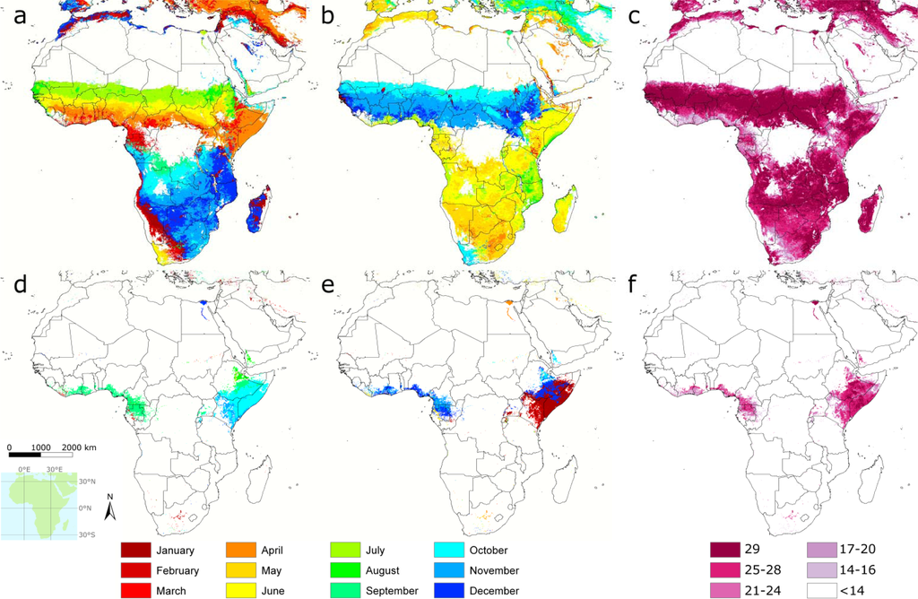
A clear gradient appears with SOS in July for the Sahel (from Mauritania to Sudan) towards earlier March–April SOS retrievals southwards, between south-east Guinea and South Sudan (Figure 1(a)). Large wetlands and irrigated areas in this region have an EOS, which extends up to three months beyond that of their surroundings (Figure 1(b)). These areas include the Inner Niger Delta near Mopti, Mali, irrigated areas south of Lake Chad (in Chad and northern Cameroon), the Gezira irrigation scheme in Sudan, and the Sudd marshes of South Sudan. The Northern and Western Cape Provinces of South Africa show a different SOS and EOS from other areas of southern Africa, which can be explained by its distinct Mediterranean climate. Large blank areas without SOS/EOS retrievals are the Sahara desert and part of the Congo Basin. Seasonality in NDVI is mostly absent in those areas. For the Congo Basin this is due to the dense tropical forest showing average NDVI values of 0.75 and above; the Sahara desert only occasionally experiences NDVI increases during rare rainstorms and has average NDVI values below 0.12.

SOS dates and their spatial patterns are similar to those found by other NDVI-phenology studies for the Sahel [24,32] and southern Africa [25], even if the NDVI time series and phenology extraction approach used may differ. In relation to season onset derived from rainfall data or estimates [33,34], our SOS retrievals occur approximately one month later. This is logical because a delay occurs between rainfall onset and vegetation green-up. Whether such a delay occurs depends however also on how rainfall onset is defined [22]. A recent study by Liebmann et al.[35] identifies the onset as the moment where daily rainfall exceeds the annual average daily rainfall: this is more similar to our 50% threshold and consequently they produce overall similar onset dates as compared to our SOS retrievals.

Large bimodal areas are identified in the Horn of Africa, and in coastal regions around the Gulf of Guinea (from Liberia to Gabon)—further referred to in this article as the Guinea Coast. For the Horn of Africa, the identified bimodal zones occur in a semi-arid climate. Between both rainy seasons, most of the vegetation senesces resulting in low NDVI values (<0.30). Bimodal rainy seasons are reported for larger areas of East Africa than visible from our analysis, for example in northern parts of Tanzania [36,37]. However, in these cases the dry spell between the short (October–December) and long rains (March–June) is generally short, and does not result in overall senescence of the vegetation. Even if multi-cropping is practiced, surrounding vegetation (trees, shrubs, pasture) remains green and abundant, thus not causing a significant lowering of NDVI values within the 8-km pixel area.

Unlike the Horn of Africa, the Guinea Coast has a tropical monsoon climate. We have two possible explanations for the observed bimodality here: (1) the bimodality is real and caused by a short relatively drier period around July–August during the long monsoon rains [38], (2) the bimodality is partially an artifact caused by reduced NDVI levels during part of the rainy season due to persistent cloud cover. This last explanation is supported by the fact that many data flags occur for this region in the NDVI3g time series, which indicate a lower quality NDVI value, i.e., NDVI data were interpolated or replaced by the average seasonal values (not shown in this article). Moreover, the bimodality is not very apparent in space and time, judging from the number of years with retrievals (Figure 1(c,f)). Given the important cloud contamination of the NDVI time series and the corresponding uncertainty for LGP retrievals, for further analysis we mask out the identified bimodal seasons in this area.

The distribution of bimodal seasons in Africa has also been evaluated from gridded rainfall and temperature products [35,39]. Liebmann et al.[35] report two annual peaks in precipitation for large areas along the Guinea Coast, which would support our first explanation given above that the bimodality in this region is real. Herrmann and Mohr [39] refer to this bimodality as a single wet season with two rainfall peaks. Both studies identify the Horn of Africa as the region with two distinct wet seasons.

Strong bimodality of the NDVI signal is also apparent in large irrigated areas. The clearest example is the Nile delta of Egypt (Figure 1) with a first season between July and September, and a second season between December and April. Another irrigated area with a clear double season is in central South Africa along the Orange and Vaal rivers, where large pivot irrigation schemes are located.

Figure 1(c,f) shows per pixel the number of years with valid phenology retrievals. For large areas we could successfully assess LGP for all years in the dataset (i.e., 29 retrievals), especially in semi-arid to sub-humid areas. Towards more arid areas, LGP is not retrieved for a number of years. This is due to the thresholds that we set on an annual basis: if average NDVI during the year becomes too low, or its dynamic range too small, LGP is not assessed. We acknowledge that in this way we do not obtain incontestable information about failed seasons that are currently classified as ‘missing data’. Nonetheless, this is not a strong limitation for the variability assessment and trend calculation of this study, if we assume that ‘missing’ seasons are equally spread over the years. In addition, in humid areas, LGP is not successfully retrieved for all years. This is especially true for areas identified as bimodal (see also discussion above). In addition, areas that we did not identify as bimodal from the long-term average NDVI profile could still show a double rainfall peak, and a more or less pronounced dry spell between these peaks depending on the year [39]. This impacts the NDVI profile and can result in strong variability of SOS/EOS retrievals, and consequently a failure to obtain seasonal parameters close to the average season.

Figure 2 shows the average LGP for both seasons, as derived from SOS and EOS (Figure 1). As stated previously, areas identified as bimodal along the Guinea Coast are masked out because these may be artifacts of cloud contamination. A similar gradient as for SOS is visible from the Sahel southwards with increasingly longer growing periods towards the south. Irrigated and wetland areas (Inner Nile Delta, Lake Chad, and Gezira scheme) have significantly longer seasons due to a later EOS. Areas with an average seasonal LGP below 90 days include the Sahelian zone, parts of Namibia and South Africa, and the Horn of Africa. This short LGP limits the potential crop choices under rainfed conditions.

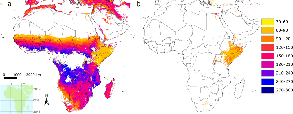
The MODIS NDVI-based LGP assessment of Butt et al.[24] for a small part of West Africa shows a similar spatial pattern as ours, although their LGP is somewhat shorter. This shorter LGP is likely due to the different phenology extraction algorithm (double-logistic function fitting), and the fact that they define EOS at the point where NDVI reaches 80% of its maximum value (this point falls earlier than our definition). Wessels et al.[25] extracted LGP for South Africa using a 20%-threshold for phenology extraction from 1-km² AVHRR NDVI data. Although coarse patterns are similar, they obtain longer season lengths in arid areas—characterized by low annual NDVI amplitudes—whereas we mask these areas due to their limited seasonality. They do acknowledge the difficulty of obtaining a good indication of LGP in these areas. Our continental LGP patterns largely correspond to patterns observed in Africa- or global-scale studies that present LGP maps [19,40], but which do not account for the occurrence of double wet seasons. A global MODIS phenology product currently exists that accounts for two seasons in one year (the Collection 5 land cover dynamics product MCD12Q2 at 500-m resolution [41]). LGP is not a standard layer and we are unaware of any studies that mapped (globally or for Africa) LGP based on this dataset. Nonetheless, LGP could easily be calculated from the contained onset and senescence dates, and future comparison of our results with this product would be of interest.

For large areas of Africa, our relatively high-resolution LGP retrievals appear to be an improvement in comparison to those derived from climate data. The last are based on sparse station data or gridded products with low accuracy in some areas (Section 1). While overall patterns are similar for Africa [5,6,42], we provide more spatial detail and separate LGP for bimodal seasons. In addition, the 30-year NDVI3g time series permit an effective assessment of LGP variability.

3.2. Variability in Length of Growing Period

Figure 3 shows the LGP variability for Africa during the 30-year period. High CV values are dominant in areas with relatively short growing periods, while low CV values correspond to long growing periods. Partly this can be explained by the fact that the CV normalizes the standard deviation by the mean, so a lower mean gives a higher CV. Nonetheless, CV is a useful measure of the LGP variability, because particularly in these short LGP areas relatively small changes in LGP can have important consequences. Not attaining the LGP in dry years may cause an incomplete crop growth cycle resulting in large yield reduction.

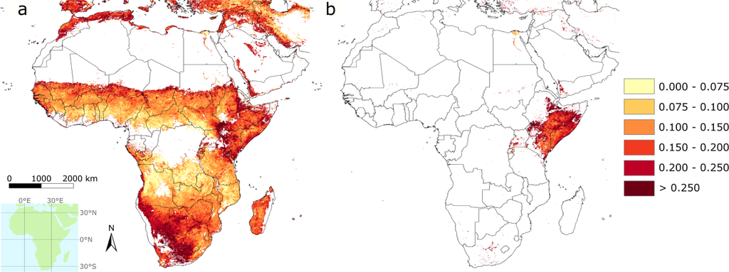
To our best knowledge, few NDVI-based studies have reported on interannual LGP variability in Africa. Two exceptions are Wessels et al.[25] for South Africa and de Jong et al.[15] at global scale. Global patterns of the variability of LGP as identified by harmonic time series analysis [15] are very similar to our Figure 3(a), although we identify some more stable regions in the Horn of Africa for individual seasons. We have not found published studies that map LGP variability over Africa as derived from climate data, although multi-annual LGP retrievals have been made [43]. The interannual variability of annual precipitation has been shown in maps, for example, [44] that indicate a higher CV in arid to semi-arid areas, corresponding to Figure 3. Among the important drivers for interannual rainfall variability in Africa, and consequently LGP, are the variable sea surface temperatures that affect wind and weather patterns [45–47]. A discussion on the drivers and impacts of climatic variability over Africa are outside the scope of this article. Instead, we refer to Brown et al.[17] for a detailed discussion on the relationship between climate indices and vegetation phenology for Africa.

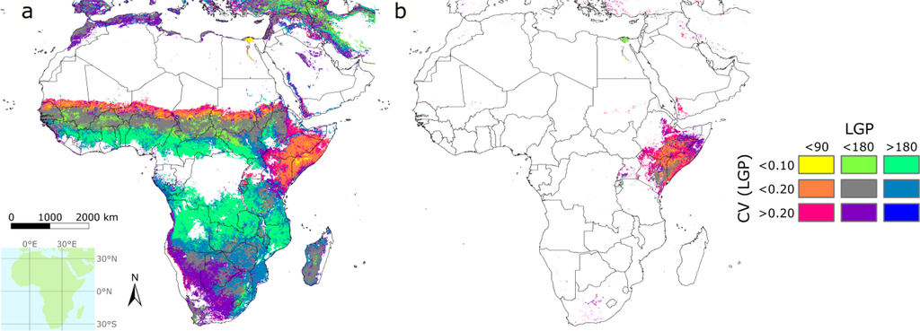
To jointly characterize mean LGP and its variability we combined Figures 2 and 3 into the bivariate maps [48] shown in Figure 4. It shows that areas with LGP below 90 days generally have a CV above 0.10. Especially towards the northern fringe of the Sahel, strong variability is apparent. Areas with LGP above 180 days have CV values below 0.20 for practically all locations. Nonetheless, these areas may also experience declining agricultural production during dry years, for example in Zimbabwe [47] that has a CV above 0.10. The main benefit of such bivariate maps is that they simultaneously provide a spatial representation of (1) which crops can be cultivated in an average year, and (2) the risk involved in cultivating these crops. This combination of factors can assist in spatially explaining the occurrence of different farming systems [49,50]. In such systems, crop choices are largely based on the potential for attaining good yields, and the risk of season failure.

3.3. Trends in Length of Growing Period

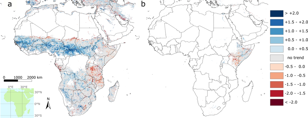
Figure 5 displays the trends in LGP that we obtained using Spearman’s rank correlation. We found significant positive LGP trends across large parts of western Africa (from Senegal to South Sudan), in parts of southern Africa, and in eastern Kenya for the long rains. Significant negative trends occur along the northern fringes of the Sahel (between Mali and Sudan), in large areas of Tanzania and northern Mozambique, and in eastern Kenya for the short rains. For the pixels with positive trends (p < 0.05) in western Africa, linear regression gives an average increase in LGP of approximately 1.13 ± 0.41 days per year, and for the eastern Kenyan long rains of 0.83 ± 0.46 days per year. For negative trends, the average reduction in LGP (in days per year) for the Sahel is 1.30 ± 0.63, for Tanzania and Mozambique 1.19 ± 0.38, and for the eastern Kenyan short rains 0.99 ± 0.45. Hence, this implies that for many areas LGP changes by more than a month over the 30-year period of the NDVI3g dataset. Although these may seem large shifts, ground reports, for example for Tanzania [51], confirm such rates of change. For pixels with significant (p < 0.10) Spearman trends, linear regression results are shown in Figure 6, indicating rates of change (days/yr). The spatial pattern of Figures 5 and 6 is the same.

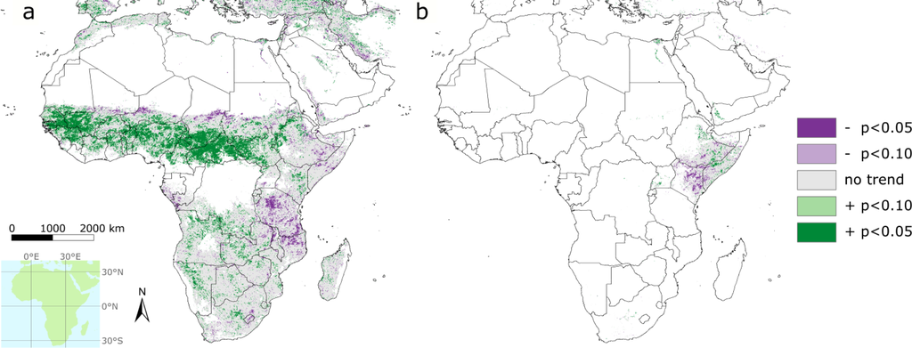
Comparison with trends in SOS and EOS (not shown here) indicates that increases in EOS dates are mostly responsible for the positive LGP trends in western Africa. Negative LGP trends in the northern fringe of the Sahel, and in Tanzania and Mozambique relate to a delay in SOS dates. Positive LGP trends for the eastern Kenyan long rains correspond to earlier SOS dates over time, while earlier EOS dates for the short rains are responsible for the decreasing length of the short rains. For eastern Kenya this seems to indicate that the dry period between short and long rains is advancing in time at the expense of the short rains.

Analyzing an earlier GIMMS version between 1981 and 2003, Julien et al.[20] also obtained negative LGP trends in Tanzania and Mozambique, and stable to slightly positive trends in western Africa. However, they did not identify negative LGP trends in the Sahel or trends for the two seasons in eastern Kenya (as they did not account for bimodality in their analysis). Similarly, Heumann et al.[23] obtained positive LGP trends in western Africa from their analysis of 1981–2005 GIMMS data, but did report negative trends for the Sahel region. Harmonic analysis of the 1981–2006 GIMMS dataset at the global scale [15] did identify negative trends in the Sahel, and positive trends in other parts of western Africa (in correspondence with our analysis although the spatial extent is somewhat different), but did not report large areas with significant trends for other parts of Africa. Differences between these studies [15,20,23] and our analysis can be explained by the phenology extraction algorithm used, whereas improvements in the current NDVI3g version over the previous GIMMS dataset could also play a role. To analyze the effect of the different length of the NDVI time series, we performed additional trend calculations for the 1981–2005 period. We found that, even if results for individual pixels changed, the above-identified regions with significant positive and negative trends were similar as for the 1981–2011 period.

Different factors can cause changes in phenology and LGP. For example if land cover changes due to human activities such as agriculture, the new vegetation cover could show a very different temporal behavior of NDVI. Climate change [46,52] and land degradation [53] are other factors that may impact phenology. In this article, we do not aim at attributing our identified LGP trends to different processes. Rather we present these trends to identify areas that merit further study given the significant trends found over large areas in our data mining exercise of the new NDVI3g dataset. We fully acknowledge that these trends should be further evaluated based on field evidence for individual locations and countries. We refer the reader to Vrieling et al.[30] for a detailed discussion on factors that may explain trends in phenology, with focus on SOS and cumulated NDVI over the season, for farming systems of Africa.

3.4. Reflections on the Phenology Extraction Approach

To extract LGP, we have used a variable threshold method [29] that we extended with a searching algorithm. In comparison to other LGP assessments, our approach gave overall good and spatially consistent results for the arid, semi-arid, and sub-humid regions of Africa. More humid areas, especially those with persistent cloud cover during specific periods of the year, generate more problems. These relate not necessarily to the method, but rather to the remaining atmospheric contamination in the NDVI series. The Guinea Coast in western and central Africa is an example of this. A potential solution could be to use vegetation optical depth retrievals from satellite passive microwave data instead of NDVI time series [54,55], although their spatial resolution is relatively coarse (approximately 0.25 degree).

We could successfully discern the areas in the Horn of Africa that experience two clearly separated wet seasons per year, as opposed to other studies that used techniques like harmonic analysis or double-logistic function fitting [15,20]. This does not mean that function-fitting is necessarily not apt for assessing phenology in bimodal areas. For example, Meroni et al.[56] extracted phenology for the Horn of Africa through function-fitting, but first determine how many maxima occur per year, which is similar to our approach. Detecting bimodality with NDVI time series will only work if two clear maxima, separated by two minima, are present in the NDVI profile. Even if short dry spells during a single season may cause a small drop in NDVI, this type of bimodality does not allow for effective separation of two LGP values per year. Such bimodality can also cause instable phenology retrievals from year to year, where otherwise a single long season becomes apparently short due to greater intensity and length of the dry spell. This instability of normal seasonal patterns from year to year (including failing of seasons or erratic dry spells during the season) may partly explain the limited years with phenological retrievals along the Guinea Coast, and in parts of Eastern Africa (Figure 1(c,f)). In this respect, an interesting classification of different types of climate modality over Africa is provided by Herrmann and Mohr [39], using gridded rainfall and temperature data.

In our current implementation of the phenology extraction method, we mask on a year-by-year basis all pixels with high mean annual NDVI, low NDVI, or with limited amplitude (Section 2.2). A negative consequence of that is that for these years our LGP series report missing data (i.e., no LGP retrieval). In some cases (Kenya, Sahel), a pixel that shows for a particular year a low mean annual NDVI or amplitude may be indicative of season failure, and thus contain important information. We identified that this may not be a strong limitation for the variability assessment and trend calculation of this study, if we assume that ‘missing’ seasons are equally spread over the years. However, for other applications information on failed seasons can be important, for example when calculating probabilities of attaining a certain LGP. This could be improved by providing separate flag values for each masking condition [56].

We have applied the variable threshold method with a local 50%-threshold, defined for each pixel and year as the average between the annual maximum and minimum NDVI. This is the same threshold value as used by White et al.[29] who argue that on average it coincides with the moment of most rapid increase and decrease in greenness (NDVI). Naturally, before the NDVI first reaches the 50% value, vegetation green-up has started, which could justify setting a lower threshold. Still when focusing on agricultural crops the 50% value seems justified, because crop emergence is usually delayed with respect to the development of surrounding natural vegetation [57]. Similarly a different threshold could be selected for EOS: in fact Rojas et al.[57] defined the end of grain filling stage as six weeks prior to EOS, with the purpose of selecting the most drought sensitive period. The same could also be achieved by setting a higher threshold value for EOS, as implemented for example in the agricultural stress index system [58]. In our view, the threshold level could be adapted, which should be informed by the purpose of analysis, or the availability of ground evidence that should be matched. Nonetheless, judging from our knowledge on Africa, the obtained SOS and EOS dates, and LGP values, our selected threshold provided realistic results.

3.5. Applications of LGP Retrievals from NDVI Time Series

Spatial LGP retrievals based on 30 years of NDVI data can benefit a number of different studies. In this section we shortly mention a few. We do not discuss here in detail the potential application of other NDVI-derived parameters. For example, Brown and de Beurs [32] already pointed to the possible replacement of current planting date estimates from gridded rainfall data with NDVI-derived SOS, in crop models like the water requirement satisfaction index [59].

Spatial assessment of LGP can help to characterize farming systems, as stated in the introduction of this paper. Currently an update to a farming systems map for Africa is under development (for the previous version see [49]). Our results, especially the combination of LGP and its CV (Figure 4), have been used as an input to spatially characterizing the limits of individual farming systems for this updated map. The main benefit of our analysis in this context is the joint spatial representation of 1) which crops can be cultivated in an average year following the mean LGP, and 2) the risk involved in cultivating these crops, as expressed by the LGP variability (Section 3.2).

LGP and its interannual variability derived from station data in Kenya have been used to predict forage production and livestock productivity [60], as these are strongly influenced by climatic variability [61]. High-resolution LGP assessment (as compared to coarser-resolution LGP derived from gridded climate data) for various years could thus help explaining the condition of livestock on a spatial and temporal basis, and add a detailed spatial dimension to field reports on livestock quality and mortality. In this way, LGP assessments could also provide insight into cattle densities and their spatial distribution during specific years.

Annual LGP assessments for longer time series permit the calculation of probabilities of not attaining an LGP of a particular length. This probability can provide information regarding chances of crop failure or livestock mortality (although trends probably need to be accounted for when determining this probability). There is an increasing attention for using satellite-based indices for micro-insurance schemes, as they can provide an objectively observed variable that correlates to production losses but cannot be influenced by the producer [62]. The index based livestock insurance project led by the International Livestock Research Institute (ILRI) is a good example [63], but many more initiatives exist. The key to success is to obtain a high correlation with agricultural production losses. This may require spatial and temporal aggregation of the satellite time series in addition to good ground data collection for several years. LGP by itself could be such an indicator that should be tested, although in areas where LGP extraction is difficult and highly variable between years (due to reasons identified in this paper) it may not be the best option. Other options include a cumulative NDVI (or another drought index) over that part of the growing period which is sensitive to droughts [64].

Even if 30 years of data by itself is too short to draw conclusions about climate change, LGP trends do inform us about ongoing phenological changes. Comparing these changes with trends obtained from climatic data could provide clues about their potential climatic forcing. The relatively high resolution of the NDVI data could in turn provide a downscaling of the effects of climatic forcing on vegetation, even for future projections. Under a wide-range of climate change scenarios, modelling studies predict a strong reduction of LGP for large parts of Africa for the next decades, especially in the semi-arid areas [42,65]. For the Sahel and parts of Eastern Africa we provide evidence that such a reduction has already started. Continuing NDVI-based spatial LGP assessments can provide ongoing evidence of this, which may complement some of the uncertainty inherent to climate models. Consistent high-quality long-term remote sensing datasets, such as the NDVI3g dataset, are a crucial input for providing converging evidence on vegetation changes. While much is to be learned regarding the human dimension of adaptation [66], such evidence is strongly needed to inform potential adaptation strategies for smallholder farmers in Africa.

4. Conclusions

We have extracted mean LGP for Africa from 30 years of AVHRR NDVI time series. Using a variable threshold method in combination with a searching algorithm, consistent results in space and time were obtained for arid, semi-arid, and sub-humid climates. Our mean LGP retrievals ranged from less than two months in arid regions up to 10 months in humid regions. To our best knowledge we are the first to report an NDVI-based LGP assessment for the full African continent that accounts for bimodality. Bimodal seasons can only be effectively discerned if two wet seasons are clearly separated, resulting in a significant reduction of NDVI. Persistent cloud cover during part of the season along the Guinea Coast may be partially responsible for the identified bimodality in that region, and hence was discarded from our analysis. Our NDVI-based LGP retrievals are a useful addition to LGP derived from climate data, as they offer higher spatial detail in areas where station data are scarce, and consequently gridded climate products are of low quality. Future comparison of our results with station-based LGP estimates can assist in optimal utilization of the complementarity between climate- and NDVI-based LGP estimates.

We determined variability and trends in LGP from a per-pixel analysis of the multi-annual LGP retrievals. A higher variability is generally found in arid and semi-arid areas, with coefficients of variation exceeding 0.25. Because not attaining a specific LGP has implications for crop development, the high variability translates into a higher risk for farmers to crop failure or reduced yields. Significant negative trends (p < 0.05) in LGP for the 30-year period were found for the northern part of the Sahel, for Tanzania and northern Mozambique, and for the short rains of eastern Kenya. Ground evidence and comparison to climatic datasets can help to understand what drives these changes. As modeling studies that use climate scenarios predict a reduction of LGP over large parts of Africa, continued monitoring of its realization is important. The 30-year NDVI3g dataset, and its future updates, are an important input for such monitoring.

We identified various applications that can benefit from our high-resolution multi-annual LGP assessment. These include the improved delineation of farming systems in Africa, spatial and temporal assessment of livestock productivity, mapping of the probability of not attaining a specific season length for example for index-based insurance schemes, and climate change studies. Although adaptations to our LGP extraction approach are possible for improved assessment at specific locations, we conclude that LGP analysis from long-term satellite time series provides useful information to study effects of climate and other change processes on vegetation and crop suitability. Such information can help to inform potential adaptation strategies to global change processes for smallholder farmers in Africa.

References

- FAO Crop Water Information: Sorghum. Available online: http://www.fao.org/nr/water/cropinfo_sorghum.html (accessed on 20 November 2012).
- Gregory, P.J.; Ingram, J.S.I.; Brklacich, M. Climate change and food security. Phil. Trans. Roy. Soc. B Biol. Sci 2005, 360, 2139–2148. [Google Scholar]
- Sarr, B. Present and future climate change in the semi-arid region of West Africa: a crucial input for practical adaptation in agriculture. Atmos. Sci. Lett 2012, 13, 108–112. [Google Scholar]
- Kruska, R.L.; Reid, R.S.; Thornton, P.K.; Henninger, N.; Kristjanson, P.M. Mapping livestock-oriented agricultural production systems for the developing world. Agr. Syst 2003, 77, 39–63. [Google Scholar]
- Fischer, G.; Nachtergaele, F.O.; Prieler, S.; Teixeira, E.; Tóth, G.; van Velthuizen, H.; Verelst, L.; Wiberg, D. Global Agro-Ecological Zones (GAEZ v3.0): Model Documentation; IIASA and FAO: Laxenburg, Austria and Rome, Italy, 2012; p. 179. [Google Scholar]
- Fischer, G.; van Velthuizen, H.; Shah, M.; Nachtergaele, F. Global Agro-Ecological Assessment for Agriculture in the 21st Century: Methodology and Results; IIASA: Laxenburg, Austria, 2002; p. 119. [Google Scholar]
- Liechti, T.C.; Matos, J.P.; Boillat, J.L.; Schleiss, A.J. Comparison and evaluation of satellite derived precipitation products for hydrological modeling of the Zambezi River Basin. Hydrol. Earth Syst. Sci. Discuss 2012, 16, 489–500. [Google Scholar]
- Maidment, R.I.; Grimes, D.I.F.; Allan, R.P.; Greatrex, H.; Rojas, O.; Leo, O. Evaluation of satellite-based and model re-analysis rainfall estimates for Uganda. Meteorol. Appl. 2013. in press. [Google Scholar]
- Ramirez-Villegas, J.; Challinor, A. Assessing relevant climate data for agricultural applications. Agr. Forest Meteorol 2012, 161, 26–45. [Google Scholar]
- de Beurs, K.M.; Henebry, G.M. Spatio-Temporal Statistical Methods for Modeling Land Surface Phenology. In Phenological Research: Methods for Environmental and Climate Change Analysis; Hudson, I.L., Keatley, M.R., Eds.; Springer: Dordrecht, The Netherlands, 2010; pp. 177–208. [Google Scholar]
- White, M.A.; de Beurs, K.M.; Didan, K.; Inouye, D.W.; Richardson, A.D.; Jensen, O.P.; O’Keefe, J.; Zhang, G.; Nemani, R.R.; van Leeuwen, W.J.D.; et al. Intercomparison, interpretation, and assessment of spring phenology in North America estimated from remote sensing for 1982–2006. Global Change Biol 2009, 15, 2335–2359. [Google Scholar]
- de Beurs, K.M.; Henebry, G.M. Land surface phenology and temperature variation in the International Geosphere-Biosphere Program high-latitude transects. Global Change Biol 2005, 11, 779–790. [Google Scholar]
- Boschetti, M.; Stroppiana, D.; Brivio, P.A.; Bocchi, S. Multi-year monitoring of rice crop phenology through time series analysis of MODIS images. Int. J. Remote Sens 2009, 30, 4643–4662. [Google Scholar]
- Vrieling, A.; De Beurs, K.M.; Brown, M.E. Recent trends in agricultural production of Africa based on AVHRR NDVI time series. Proc. SPIE 2008, 7104, 71040R–71040R-10. [Google Scholar]
- de Jong, R.; de Bruin, S.; de Wit, A.; Schaepman, M.E.; Dent, D.L. Analysis of monotonic greening and browning trends from global NDVI time-series. Remote Sens. Environ 2011, 115, 692–702. [Google Scholar]
- Reed, B.C.; Schwartz, M.D.; Xiao, X. Remote Sensing Phenology: Status and the Way Forward. In Phenology of Ecosystem Processes : Applications in Global Change Research; Noormets, A., Ed.; Springer-Verlag: New York, NY, USA, 2009; pp. 231–246. [Google Scholar]
- Brown, M.E.; de Beurs, K.M.; Vrieling, A. The response of African land surface phenology to large scale climate oscillations. Remote Sens. Environ 2010, 114, 2286–2296. [Google Scholar]
- Tucker, C.J. Red and photographic infrared linear combinations for monitoring vegetation. Remote Sens. Environ 1979, 8, 127–150. [Google Scholar]
- Moulin, S.; Kergoat, L.; Viovy, N.; Dedieu, G. Global-scale assessment of vegetation phenology using NOAA/AVHRR satellite measurements. J. Clim 1997, 10, 1154–1170. [Google Scholar]
- Julien, Y.; Sobrino, J.A. Global land surface phenology trends from GIMMS database. Int. J. Remote Sens 2009, 30, 3495–3513. [Google Scholar]
- Zhang, X.; Friedl, M.A.; Schaaf, C.B.; Strahler, A.H.; Liu, Z. Monitoring the response of vegetation phenology to precipitation in Africa by coupling MODIS and TRMM instruments. J. Geophys. Res.-Atmos 2005, 110, D12103. [Google Scholar]
- Groten, S.M.E.; Ocatre, R. Monitoring the length of the growing season with NOAA. Int. J. Remote Sens 2002, 23, 2797–2815. [Google Scholar]
- Heumann, B.W.; Seaquist, J.W.; Eklundh, L.; Jönsson, P. AVHRR derived phenological change in the Sahel and Soudan, Africa, 1982–2005. Remote Sens. Environ 2007, 108, 385–392. [Google Scholar]
- Butt, B.; Turner, M.D.; Singh, A.; Brottem, L. Use of MODIS NDVI to evaluate changing latitudinal gradients of rangeland phenology in Sudano-Sahelian West Africa. Remote Sens. Environ 2011, 115, 3367–3376. [Google Scholar]
- Wessels, K.; Steenkamp, K.; von Maltitz, G.; Archibald, S. Remotely sensed vegetation phenology for describing and predicting the biomes of South Africa. Appl. Veg. Sci 2011, 14, 49–66. [Google Scholar]
- Pinzón, J.E. Revisiting error, precision and uncertainty in NDVI AVHRR data: Development of a consistent NDVI3g time series. Remote Sens 2013. in preparation. [Google Scholar]
- Savitzky, A.; Golay, M.J.E. Smoothing and differentiation of data by simplified least squares procedures. Anal. Chem 1964, 36, 1627–1639. [Google Scholar]
- Chen, J.; Jönsson, P.; Tamura, M.; Gu, Z.; Matsushita, B.; Eklundh, L. A simple method for reconstructing a high-quality NDVI time-series data set based on the Savitzky-Golay filter. Remote Sens. Environ 2004, 91, 332–344. [Google Scholar]
- White, M.A.; Thornton, P.E.; Running, S.W. A continental phenology model for monitoring vegetation responses to interannual climatic variability. Glob. Biogeochem. Cy 1997, 11, 217–234. [Google Scholar]
- Vrieling, A.; de Beurs, K.M.; Brown, M.E. Variability of African farming systems from phenological analysis of NDVI time series. Climatic Change 2011, 109, 455–477. [Google Scholar]
- Spearman, C. The proof and measurement of association between two things. Am. J. Psychol 1904, 15, 72–101. [Google Scholar]
- Brown, M.E.; de Beurs, K.M. Evaluation of multi-sensor semi-arid crop season parameters based on NDVI and rainfall. Remote Sens. Environ 2008, 112, 2261–2271. [Google Scholar]
- Laux, P.; Kunstmann, H.; Bardossy, A. Predicting the regional onset of the rainy season in West Africa. Int. J. Climatol 2008, 28, 329–342. [Google Scholar]
- Tadross, M.A.; Hewitson, B.C.; Usman, M.T. The interannual variability on the onset of the maize growing season over South Africa and Zimbabwe. J. Clim 2005, 18, 3356–3372. [Google Scholar]
- Liebmann, B.; Blade, I.; Kiladis, G.N.; Carvalho, L.M.V.; Senay, G.B.; Allured, D.; Leroux, S.; Funk, C. Seasonality of African Precipitation from 1996 to 2009. J. Clim 2012, 25, 4304–4322. [Google Scholar]
- Vrieling, A.; Sterk, G.; Vigiak, O. Spatial evaluation of soil erosion risk in the West Usambara Mountains, Tanzania. Land Degrad. Dev 2006, 17, 301–319. [Google Scholar]
- Zorita, E.; Tilya, F.F. Rainfall variability in Northern Tanzania in the March–May season (long rains) and its links to large-scale climate forcing. Clim. Res 2002, 20, 31–40. [Google Scholar]
- Windmeijer, P.N.; Andriesse, W. Inland Valleys in West Africa: An Agro-Ecological Characterization of Rice-Growing Environments; International Institute for Land Reclamation and Improvement (ILRI): Wageningen, The Netherlands, 1993; p. 160. [Google Scholar]
- Herrmann, S.M.; Mohr, K.I. A continental-scale classification of rainfall seasonality regimes in Africa based on gridded precipitation and land surface temperature products. J. Appl. Meteorol. Clim 2011, 50, 2504–2513. [Google Scholar]
- HarvestChoice Measuring Growing Seasons, Available online: http://harvestchoice.org/labs/measuring-growing-seasons (accessed on 26 November 2012).
- Ganguly, S.; Friedl, M.A.; Tan, B.; Zhang, X.Y.; Verma, M. Land surface phenology from MODIS: Characterization of the Collection 5 global land cover dynamics product. Remote Sens. Environ 2010, 114, 1805–1816. [Google Scholar]
- Thornton, P.K.; Jones, P.G.; Owiyo, T.; Kruska, R.L.; Herrero, M.; Kristjanson, P.; Notenbaert, A.; Bekele, N.; Omolo, A. Mapping Climate Vulnerability and Poverty in Africa. Report to the Department for International Development; ILRI: Nairobi, Kenya, 2006; p. 171. [Google Scholar]
- FAO Global Agro-Ecological Zones Data Portal version 3. Available online: http://gaez.fao.org/ (accessed on 18 January 2013).
- von Wehrden, H.; Hanspach, J.; Kaczensky, P.; Fischer, J.; Wesche, K. Global assessment of the non-equilibrium concept in rangelands. Ecol. Appl 2012, 22, 393–399. [Google Scholar]
- Janicot, S.; Trzaska, S.; Poccard, I. Summer Sahel-ENSO teleconnection and decadal time scale SST variations. Clim. Dynam 2001, 18, 303–320. [Google Scholar]
- Giannini, A.; Biasutti, M.; Held, I.M.; Sobel, A.H. A global perspective on African climate. Climatic Change 2008, 90, 359–383. [Google Scholar]
- Nicholson, S.E.; Webster, P.J. A physical basis for the interannual variability of rainfall in the Sahel. Q. J. Roy. Meteorol. Soc 2007, 133, 2065–2084. [Google Scholar]
- Teuling, A.J.; Stöckli, R.; Seneviratne, S.I. Bivariate colour maps for visualizing climate data. Int. J. Climatol 2011, 31, 1408–1412. [Google Scholar]
- Dixon, J.; Gulliver, A.; Gibbon, D. Farming Systems and Poverty: Improving Farmers’ Livelihoods in a Changing World; FAO, Rome and World Bank: Washington, DC, USA, 2001; p. 412. [Google Scholar]
- Seré, C.; Steinfeld, H. World Livestock Production Systems: Current Status, Issues and Trends; FAO Animal Production and Health Paper 127; FAO: Rome, Italy, 1995. [Google Scholar]
- Lema, M.A.; Majule, A.E. Impacts of climate change, variability and adaptation strategies on agriculture in semi arid areas of Tanzania: the case of Manyoni District in Singida Region, Tanzania. Afr. J. Environ. Sci. Tech 2009, 3, 206–218. [Google Scholar]
- Scheiter, S.; Higgins, S.I. Impacts of climate change on the vegetation of Africa: An adaptive dynamic vegetation modelling approach. Global Change Biol 2009, 15, 2224–2246. [Google Scholar]
- Zika, M.; Erb, K.-H. The global loss of net primary production resulting from human-induced soil degradation in drylands. Ecol. Econ 2009, 69, 310–318. [Google Scholar]
- Jones, M.O.; Jones, L.A.; Kimball, J.S.; McDonald, K.C. Satellite passive microwave remote sensing for monitoring global land surface phenology. Remote Sens. Environ 2011, 115, 1102–1114. [Google Scholar]
- Jones, M.O.; Kimball, J.S.; Jones, L.A.; McDonald, K.C. Satellite passive microwave detection of North America start of season. Remote Sens. Environ 2012, 123, 324–333. [Google Scholar]
- Meroni, M.; Verstraete, M.; Urbano, F.; Rembold, F.; Kayitakire, F. Phenology-Tuned Biomass Production Anomaly Detection for Food Security Monitoring: Methods and Application to the Case Study of the Horn of Africa (oral presentation). Proceedings of 1st EARSeL Workshop on Temporal Analysis of Satellite Images, Mykonos Island, Greece, 23–25 May 2012.
- Rojas, O.; Vrieling, A.; Rembold, F. Assessing drought probability for agricultural areas in Africa with coarse resolution remote sensing imagery. Remote Sens. Environ 2011, 115, 343–352. [Google Scholar]
- van Hoolst, R.; Eerens, H.; Bydekerke, L.; Rojas, O.; Racionzer, P.; Rembold, F.; Vrieling, A. Development of a Global Agricultural Stress Index System (ASIS) Based on Remote Sensing Data. Proceedings of 1st EARSeL Workshop on Temporal Analysis of Satellite Images, Mykonos Island, Greece, 23–25 May 2012.
- Verdin, J.; Klaver, R. Grid-cell-based crop water accounting for the famine early warning system. Hydrolog. Process 2002, 16, 1617–1630. [Google Scholar]
- Bekure, S.; de Leeuw, P.N.; Nyambaka, R. The Long-Term Productivity of the Maasai Livestock Production System. In Maasai Herding: An Analysis of the Livestock Production System of Maasai Pastoralists in Eastern Kajiado District Kenya; Bekure, S., de Leeuw, P.N., Grandin, E.E., Neate, P.J.H., Eds.; ILCA: Addis Ababa, Ethiopia, 1991; pp. 127–140. [Google Scholar]
- Stige, L.C.; Stave, J.; Chan, K.S.; Ciannelli, L.; Pettorelli, N.; Glantz, M.; Herren, H.R.; Stenseth, N.C. The effect of climate variation on agro-pastoral production in Africa. Proc. Natl. Acad. Sci. USA 2006, 103, 3049–3053. [Google Scholar]
- Makaudze, E.M.; Miranda, M.J. Catastrophic drought insurance based on the remotely sensed normalised difference vegetation index for smallholder farmers in Zimbabwe. Agrekon 2010, 49, 418–432. [Google Scholar]
- Chantarat, S.; Mude, A.G.; Barrett, C.B.; Carter, M.R. Designing Index-Based Livestock Insurance for Managing Asset Risk in Northern Kenya. J. Risk Insur. 2013. in press. [Google Scholar]
- Rojas, O. Operational maize yield model development and validation based on remote sensing and agro-meteorological data in Kenya. Int. J. Remote Sens 2007, 28, 3775–3793. [Google Scholar]
- Thornton, P.K.; Jones, P.G.; Ericksen, P.J.; Challinor, A.J. Agriculture and food systems in sub-Saharan Africa in a 4 degrees C+ world. Phil. Trans. Math. Phys. Eng. Sci 2011, 369, 117–136. [Google Scholar]
- Ericksen, P.J.; Ingram, J.S.I.; Liverman, D.M. Food security and global environmental change: emerging challenges. Environ. Sci. Pol 2009, 12, 373–377. [Google Scholar]