Abstract
The objective of the research is to characterize the surface spectral reflectance of the nearshore waters using atmospheric correction code—Tafkaa for retrieval of the marine water constituent concentrations from hyperspectral data. The study area is the nearshore waters of New York/New Jersey considered as a valued ecological, economic and recreational resource within the New York metropolitan area. Comparison of the Airborne Visible Infrared Imaging Spectrometer (AVIRIS) measured radiance and in situ reflectance measurement shows the effect of the solar source and atmosphere in the total upwelling spectral radiance measured by AVIRIS. Radiative transfer code, Tafkaa was applied to remove the effects of the atmosphere and to generate accurate reflectance (R(0)) from the AVIRIS radiance for retrieving water quality parameters (i.e., total chlorophyll). Chlorophyll estimation as index of phytoplankton abundance was optimized using AVIRIS band ratio at 675 nm and 702 nm resulting in a coefficient of determination of R2 = 0.98. Use of the radiative transfer code in conjunction with bio optical model is the main tool for using ocean color remote sensing as an operational tool for monitoring of the key nearshore ecological communities of phytoplankton important in global change studies.
1. Introduction
The aim of an algorithm based on radiative transfer theory (RTT) is a physical-bio-optical description of the radiative transfer process in the entire system from the solar source to the remote sensor via the hydrosols. The quantitative description provides a sound basis for the inversion of remotely sensed signals to retrieve the optical water quality parameters (i.e., total chlorophyll or total suspended material) [1]. Algorithms for retrieving the chlorophyll concentration from space have been developed for sensors such as CZCS (coastal Zone Color Scanner), SeaWiFS (the Sea-viewing Wide Field-view Sensor), MODIS (Moderate-Resolution Imaging Spectroradiometer) and others [2]. However, most of these algorithms have been applied mainly to the case 1 (oceanic) waters. These algorithms usually include two steps. The first step is the atmospheric correction, which is applied to separate the atmospheric radiance from the water-leaving radiance. The next step is based on a bio-optical model to relate the water-leaving radiance to the water constituent concentration. Because the water-leaving radiance typically comprises at most about 10% of the total radiance at the top of the atmosphere (TOA), the key to reliable retrieval of the water-leaving radiance from the measured total radiance is an accurate correction of the effects of aerosol scattering and absorption [3]. NASA Airborne Visible-Infrared Imaging Spectrometer (AVIRIS) records the integrated effects of the solar source, the atmosphere and the targeted surface. To compensate for the atmospheric effects an air-water interface atmospheric correction algorithm—Tafkaa [4] was applied to AVIRIS data to infer the water-leaving radiance. This paper reports on the ongoing research using the data from the AVIRIS imaging spectrometer, field spectroradiometer and water samplings [5,6]. Based on these measurements optical water quality models are constructed to establish the relationship between concentrations and atmospherically corrected optical measurements recorded by the AVIRIS. The high spatial/spectral resolution of the AVIRIS data is advantageous for coastal water property retrieval which is characterized by high spatial/temporal variation. To validate the performance of the Tafkaa, the water samplings collected simultaneously with AVIRIS overflight (May 15, 2000) and complemented with additional field data (May 8, 2000) from the same sampling locations were compared with Tafkaa derived reflectance spectra both visually and quantitatively. The regression analysis identified a strong relationship (R2 = 0.98 and P < 0.001), between the estimated chlorophyll from atmospherically corrected AVIRS band ratio and field measured values of chlorophyll concentrations. This result provides a baseline reference essential for future processing and analysis of the atmospherically corrected hyperspectral data in nearshore waters.
2. Materials and Methods
A brief description of the research material and method as related to the output results derived from Tafkaa is given below to evaluate the utility of Tafkaa in hyperspectral data analysis. Detailed descriptions on laboratory analysis and the establishment of the bio optical model of the estuary can be found in Bagheri et al., 2000, 2005 and 2008.
2.1. Study Area
The study area is the Hudson/Raritan Estuary located south of the Verrazano Narrows and bordered by western Long Island, Staten Island and New Jersey (Figure 1). The estuary is a partially mixed drowned river estuary [7] and it is relatively shallow (<8 m). The slow estimated flushing time of the estuary, 16–21 days or 32 to 42 tidal cycles [8], tends to retain pollutants entering the system and delay dilution with receiving waters. Over the last century the quality of the estuarine water has degraded in part due to eutrophication which disrupts the pre-existing natural balance of the system, resulting in phytoplankton blooms of both increased frequency and intensity in response to the over-enrichment of nutrients [9]. It is imperative, because of the damage to aquatic ecosystems, fisheries and tourism, that the environmental conditions that trigger and control blooms of harmful algae be sufficiently understood in order to predict occurrences and mitigate potential effects. The sampling stations marked on Figure 1 are located where the effect of bottom reflectance recorded by the Secchi disk readings (collected simultaneously with AVIRIS overflight on May 15, 2000) is minimum (0.6 m) and the taxonomic variability in phytoplankton community is maximum [5]. The sample locations correspond to the locations of the AVIRIS Transects (T1, 2 and 3) acquired on May 15, 2000. The focus of this paper is the AVIRIS Transect 3 (T3) covering the Sandy Hook segment of the Hudson/Raritan Estuary.
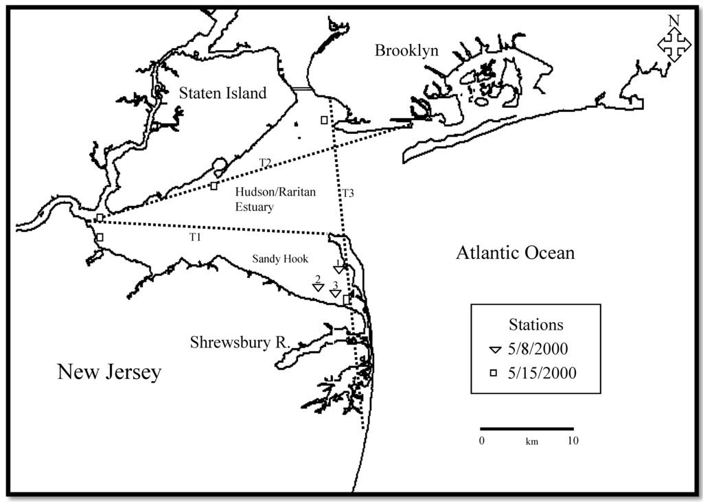
Figure 1.
Map of the study area with the samplings (1,2,3) and transects locations(T 1,2,3).
Figure 1.
Map of the study area with the samplings (1,2,3) and transects locations(T 1,2,3).

2.2. Sensors and Data Characteristics
2.2.1. AVIRIS
AVIRIS hyperspectral data (Table 1) in conjunction with simultaneous in-water measurements using the field spectroradiometer and shipboard samplings were collected in Hudson/Raritan Estuary of NY-NJ on May 15, 2000. Calibrated AVIRIS data was provided by the AVIRIS project office at the NASA Jet Propulsion Laboratory. AVIRIS records the integrated effects of the solar source, the atmosphere and the targeted surface. Thus the data needs to be corrected for atmospheric effects in order to infer the water leaving radiance.

Table 1.
Specification of AVIRIS.
| Sensor Design | Whisk broom, 4 spectrometers |
| Platform | Airborne ER-2 @~20 km |
| Spectral Characteristics | 224 bands, ∆λ ~ 10 nm, FWHM ~ 10 nm, range 375–2,500 nm |
| Typical GSD | ~20 m from ER-2 |
| Full field of view | 30° (~12 km at ER-2 altitude) |
| SWIR Characteristics | Relatively high SNR |
2.2.2. Field Spectroradiometer—OL 754
Optronic Laboratory (OL 754) is a scanning, submersible spectroradiometer, which makes spectral measurements in 300–850 nm at wavelength resolutions from 1 nm to 10 nm for computation of normalized percentage reflectance curves. Upwelling (Eu(λ)) and downwelling (Ed(λ)) irradiances were measured and used to calculate the subsurface irradiance reflectance R(0−) or water leaving radiance for comparison with modeled reflectance derived from inherent optical properties (IOPs). The measurements of up/downward light fields and associated parameters (fraction of diffuse skylight, etc.) were used to establish the correlation between geometrically/atmospherically corrected AVIRIS data and “in water” measurements at designated sample locations within the study site (Figure 1). Locations of the sample points were recorded using the GPS onboard the ship for correlation with georeferenced image data.
2.2.3. Shipboard Samplings
Shipboard Samplings (i.e., water sampling and optical measurements) were coordinated during the AVIRIS data acquisition (May 15, 2000) and complemented with additional sampling taken from the same station locations within the estuary (May 8, 2000). Standard procedures were used to determine the concentrations of total chlorophyll (TCHL) (as indication of concentration of phytoplankton) and total suspended matter (TSM) (NEN 6520 (1981)) and NEN 6484 (1982)) respectively. The TCHL concentrations varied between 44 mg m−3 and 6 mg m−3 indicating that the measurements did not coincide with any major outbreaks of phytoplankton blooms in the estuary. Likewise, the TSM ranges (17–5 g m−3) were within the expected values for the time of year when the measurements taken.
2.2.4. Inherent Optical Properties (IOPs)
IOPs measured directly include spectral absorption (a) and spectral beam attenuation (c), using Ocean Optics-2000 spectrometer. Spectral scattering (b) was then deduced via subtraction of absorption from the beam attenuation; (b = c − a). The samples were also analyzed for identification/enumeration of the phytoplankton species to demonstrate the variety and composition of phytoplankton populations for input into library spectra of phytoplankton in the Hudson/Raritan Estuary.
2.3. Bio-Optical Model
A simple optical water quality model based on the work of Gordon et al., [10] was calibrated on measurements of optical water constituent concentrations and inherent optical properties and were used to simulate subsurface irradiance reflectance (or water leaving radiance):
where a is the total absorption coefficient, bb is the backscatter coefficient, and r is a factor based on the geometry of incoming light and volume scattering in the water, and all quantities are understood as functions of wavelength. Furthermore,
where:
R(0−) = r (bb/(a + bb))
a = aw + a*TSM [TSM] + a*ph[CHL] + a*CDOM[CDOM440]
bb = 0.5•bw + bb*TSM[TSM]
- aw = absorption of pure water,
- bw = scattering of pure water,
- a*ph = specific absorption of the phytoplankton,
- bb*TSM = specific backscatter of TSM (Total Suspended Material),
- a*TSM = specific absorption of TSM,
- 0.5 = backscatter to scatter ratio of pure water,
- a*CDOM = specific absorption of CDOM (Color Dissolved Organic Matter).
Here, [TSM] represents the concentration of the total suspended material, [CHL] represents the concentration of chlorophyll, and [CDOM440] is the absorption due to CDOM at 440 nm. The asterisks denote that a and bb are specific inherent optical properties per unit concentration denoted by the subscript.
Using the bio-optical model, R(0−) spectra were simulated for the measured concentrations (using measured IOPs). Comparison of simulated and measured R(0−) provided a means to validate the bio-optical model and its accuracy as compared with the in situ R(0−) measurements recorded by the field spectroradiometer [6]. Subsequently these spectra were used to validate the performance of Tafkaa, in atmospheric correction of AVIRIS as detailed in the “result and discussion” section of this paper.
2.4. Atmospheric Correction
The remote sensing signal received by the AVIRIS is the sum of the water-leaving radiance and contribution from atmospheric aerosols and molecules. Most of the atmospheric correction algorithms are designed for case 1 (oceanic) water and are based on the assumption that the water-leaving radiances are close to zero in the spectral range 760–870 nm. Thus, an aerosol model and an aerosol optical depth can be derived from the bands located in that region of the spectrum. Subsequently, the aerosol information can be extrapolated into the visible range for retrieval of the water-leaving radiance and the water constituent concentration. Unfortunately, these algorithms are not directly applicable to case 2 (turbid coastal) waters because of the presence of suspended materials which cause strong scattering in the spectral range 760–870 nm. These bands are not suitable for aerosol retrieval in the coastal water, because of the strong scattering of coastal water in those wavelengths. In atmospheric correction, the most challenging issue is to remove the impact of the aerosol component on top of the atmosphere (TOA) to convert remote sensing measured radiance into water leaving radiance. This is the required input to algorithms designed to retrieve chlorophyll-a as indication of phytoplankton or suspended material concentrations. Tafkaa input parameters derived from the AVIRIS metadata file is listed in Table 2. A full description of these and other input parameters (i.e., solar and viewing geometry) can be found in Tafkaa User’s Guide [11]. Tafkaa is an extensively modified version of the Atmospheric REMoval algorithm (ATREM) [12] that has been specifically adapted to address the confounding variables associated with aquatic remote sensing applications [13] and [14].
Table 2.
Tafkaa atmospheric parameters applied to AVIRIS (5/15/2000).
| Parameter | Parameterization | Source |
|---|---|---|
| Input radiance data cube | Image centre latitude = 40°44′00″ Image centre longitude = 73°53′50″ | AVIRIS Jet Propulsion Laboratory |
| Cloud mask | NDVI > 0.05 | AVIRIS Input data cube |
| Atmospheric Model | Mid-Latitude Summer | Selected from MODTRAN standard models (based on the surface temperatures) |
| Ozone | 0.325 | Acquired from Earth Probe TOMS (Total Ozone Mapping Radiometer) |
| Atmospheric Gases | H2O, CO2, O3, CO, CH4, O2 | Tafkaa options |
| Geometry | Single nadir viewing: Image centre zenith angle = 45°00′00″ | Calculated from AVIRIS header data |
| Image centre azimuth angle = 194°00′00″ | ||
| Aerosol method | Pixel-by-pixel | Tafkaa options |
| Aerosol model | Coastal | Selected from MODTRAN standard models based on geography of the scene |
| Relative Humidity | 80% | Tafkaa options (selection on the basis of weather of the day) |
| Aerosol wavelengths | 0.86, 1.04 | Tafkaa options (selection based on the quality of the radiance cube. excluding noisy bands) |
| Exclude aerosol model | none | Tafkaa options (based on the scene geography) |
| Exclude relative humidity | 90%, 98% | Tafkaa options (based on the scene geography) |
| Sensor altitude | 20.16 (km) | Acquired AVIRIS header data |
| Wind speed | 2 (m/s) |
3. Results and Discussion
Comparison of AVIRIS measured radiance and in situ reflectance revealed the effects of the atmosphere on the total upwelling radiance measured by AVIRIS. Tafkaa was used to calculate the amount of light incident above the water surface (downwelling irradiance) for AVIRIS hyperspectral data using a coastal aerosol model, with all available gaseous absorption calculations (H2O, CO2, O3, N2O, CO, CH4, O2).
Tafkaa was run with a mid-latitude summer atmospheric model, using the 940 and 1,140 nm bands to derive water vapor, allowing the model to estimate atmospheric visibility based on image characteristics. Options were also selected to reduce the effects of spectral mismatch and minimize the errors associated with the water vapor bands and other smaller spectral artifacts [15]. Tafkaa output (in reflectance units) is used to provide the link between the spectra measured by the AVIRIS spectrometers and the “in water” measurements of spectral reflectance using the field spectroradiometer by considering the effect of aerosol scattering in the 400 to 700 nm region with an increasing effect toward shorter wavelengths. The air-water effects were taken into account comparing Tafkaa derived AVIRIS (R(0) with field spectroradiometer R(0−) below the surface of water [16]. Figure 2 shows the comparison of the in situ reflectance R(0−) measured “in-water” and atmospherically corrected AVIRIS reflectance R(0) derived from Tafkaa for sample station 1 marked on Figure 1.

Figure 2.
Comparison of reflectance spectra measured by the field spectroradiometer (OL754) and Tafkaa derived AVIRIS spectra for sampling station 1 (Figure 1). (Note: The “in-water” measured spectra are produced by a submersible spectroradiometer as point location and Tafkaa derived reflectance spectra are based on AVIRIS data with spatial resolution of 20 m × 20 m).
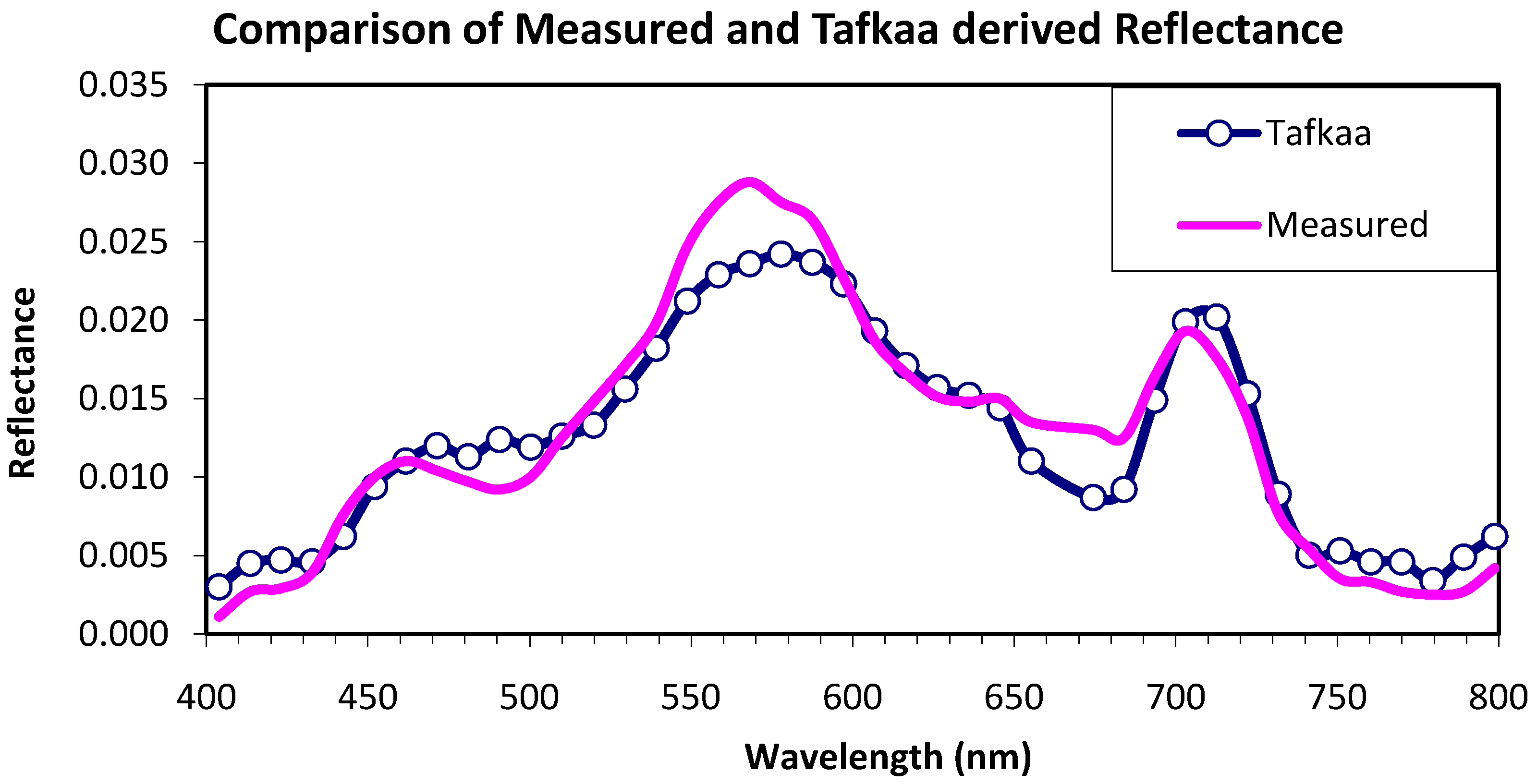
As expected, reflectance values in the Tafkaa output tend to approach zero at longer wavelengths. The general shape of the Tafkaa derived reflectance spectra and the range of values seems to be realistic for 450–750 nm with the spectral maximum observed around 550–600 nm. Thus algorithms based on phytoplankton optical properties in the red wavelength region (near 675 nm coinciding with the 2nd chlorophyll absorption peak) are preferred since they provide better basis for remote monitoring of phytoplankton blooms in Case 2 waters. This is due to minimum interference from color dissolved organic material (CDOM) in this wavelength region while its maximum interference around 440 nm coincides with the 1st chlorophyll absorption peak. Although a certain amount of spectral mismatch is evident in the results (e.g., around the 680 nm), overall, the Tafkaa derived spectra are reasonable for those locations sampled in situ and marked on Figure 1. As stated before, the “in water” measured R(0−) spectra were used to validate atmospherically corrected AVIRIS observations of reflectance spectra. Figure 3 shows the comparison of measured R(0−) spectra for stations 2 and 3 with different levels of chlorophyll concentrations as calculated in the laboratory with Tafkaa derived AVIRIS reflectance spectra for the corresponding stations.
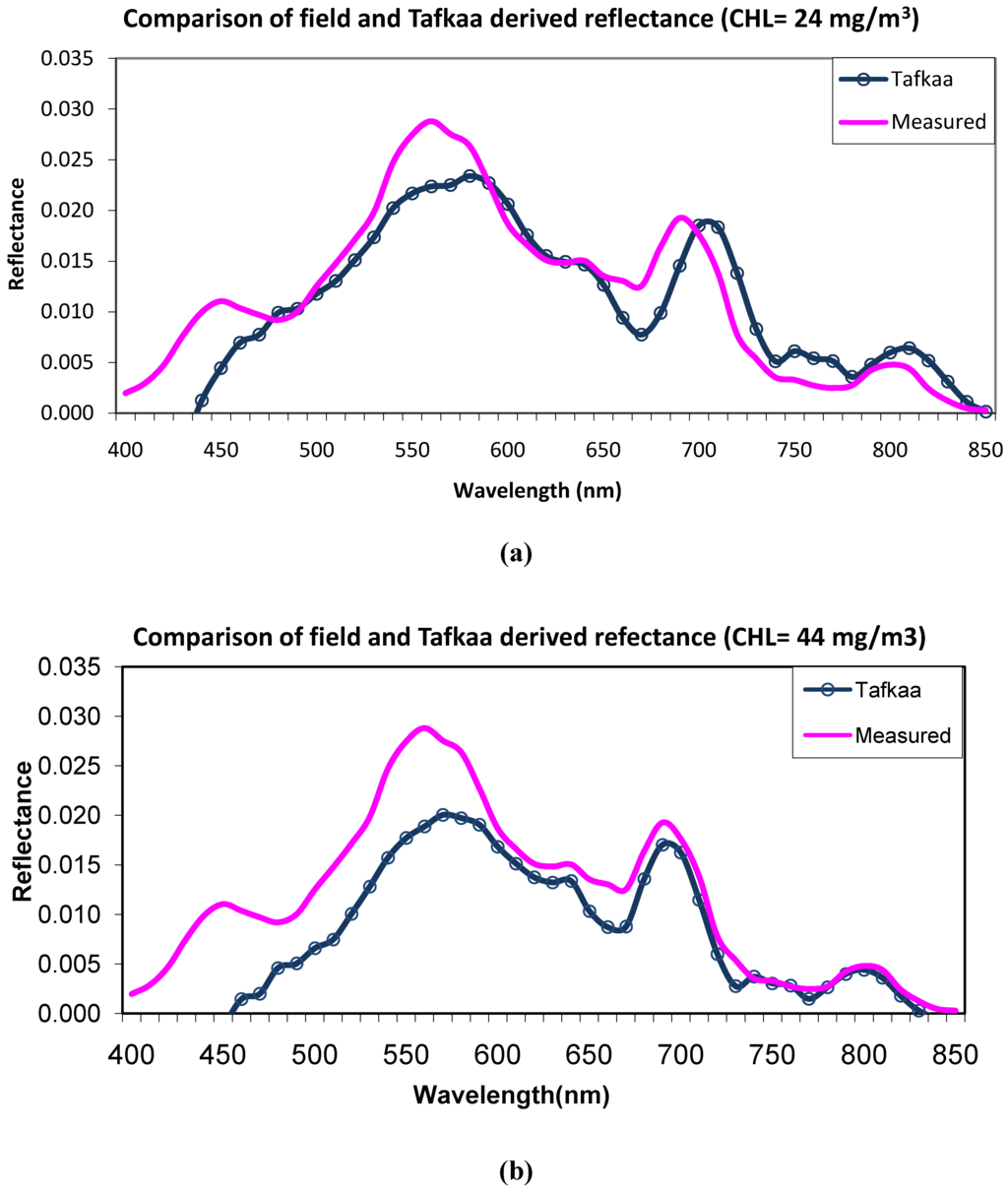
Figure 3.
Comparisons of measured spectra for station 2 (a) and station 3 (b) with different chlorophyll concentrations and Tafkaa derived AVIRIS reflectance spectra for the corresponding sampling stations (see Figure 1).
Figure 3.
Comparisons of measured spectra for station 2 (a) and station 3 (b) with different chlorophyll concentrations and Tafkaa derived AVIRIS reflectance spectra for the corresponding sampling stations (see Figure 1).
ENVI software was used for image processing including georeferencing of the AVIRIS and band ratio analysis. Satellite remote sensing (i.e., CZCS, SeaWIFS and MODIS) data and associated reflectance (R) ratios have been applied to monitor chlorophyll in case 1 waters [2] and [17]. In inland water, [18] determined that the ratio of AVIRIS bands around 705 nm with the band at 677 nm was the most sensitive for detecting chlorophyll-a and it is applicable for retrieval of chlorophyll concentrations in a wide range of case 2 waters. The advantage of using the ratio of spectral radiance reflectance is all of the backscattering coefficients can be ignored. In other words, the ratio can be expressed by using only absorption coefficients, which are more stable for measurement than backscattering coefficients [19].
Using Equation 4 [18], a similar band ratio (702 nm and 675 nm) was applied to Tafkaa derived AVIRIS data of T3. The model was parameterized using measured IOPs of Hudson/Raritan estuarine waters [6] representing the optical characteristics of the estuarine waters.
Estimated Chlorophyll = 90.035(R (0)675/R (0)702) − 70.108
The two wavelengths selected were close: one within the absorption range of chlorophyll-a, and the other one outside of the absorption range in order to estimate the chlorophyll-a concentration more accurately. The wavelengths selected found to be close to the published literature and are calibrated with shipboard data collected in this geographic location. The establishment of the “wavelengths” in band ratio technique is important for better estimation when the chlorophyll concentration is relatively low. Figure 4 is a thematic map of ratio image which depicts the spatial distribution of chlorophyll concentration. The concentrations for given pixels of the Tafkaa derived AVIRIS data are consistent with in situ data supporting the validity of the approach.
The ratio image map (Figure 4) shows maximum values of chlorophyll concentration in the Shrewsbury River and its confluence with the estuarine water (Figure 1). These maps are important input into a geographic information system (GIS) for better monitoring and management of water resources. Overall, Tafkaa produced more acceptable output result for atmospheric correction when compared to the earlier result generated by other (e.g., MODTRAN) atmospheric correction code using AVIRIS [20]. This comparison is not perfect since analysis of spatial and temporal changes within and between AVIRIS transects need to be performed with greater confidence that differences are a function of changing water characteristics and not artifacts of atmospheric correction code.
Likewise, the regression analysis identified a strong relationship (R2 = 0.98) between the estimated chlorophyll concentrations derived from the AVIRIS band ratio (Figure 4) and laboratory measured values (for sample stations located along T3 on Figure 1). The statistical summary and graph (Figure 5) of the regression analysis as shown below indicate that the model is most useful in the vicinity of the (,) value on the regression line:
- Intercept = −6.08
- Slope = 1.08
- Variance of the Error = 6.372219
- Root Mean Square Error = 1.12891
- P-value = 0.001365
- Correlation Coefficient = 0.9783

Figure 4.
Spatial distribution of chlorophyll concentration based on band ratio of AVIRIS atmospherically corrected data covering Sandy Hook segment of Transect 3 (T3 on Figure 1).
Figure 4.
Spatial distribution of chlorophyll concentration based on band ratio of AVIRIS atmospherically corrected data covering Sandy Hook segment of Transect 3 (T3 on Figure 1).
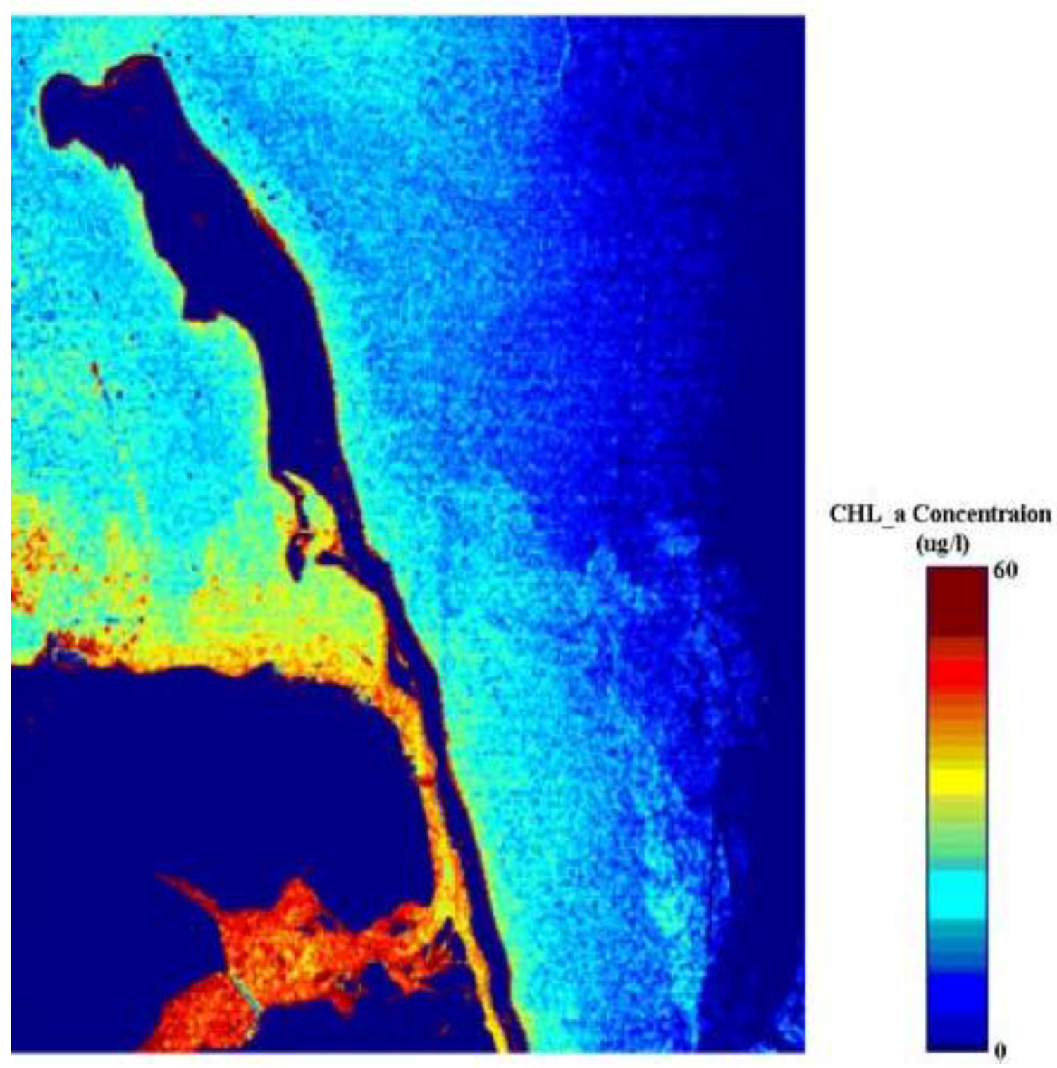
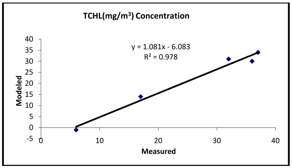
Figure 5.
Trend line for the given values of measured and calculated chlorophyll concentration.
Figure 5.
Trend line for the given values of measured and calculated chlorophyll concentration.

Utilizing regression, the aim was to generate the calibration factor without the statistical requirements (i.e., use of a large number of sample points). The data fits well into the model and if more information is needed, a case study for every value of the independent variable can be performed. The result is valuable providing a baseline reference for future processing and analysis of the atmospherically corrected hyperspectral data in coastal/estuarine waters.
4. conclusions
The high spatial/spectral resolution of the AVIRIS data is advantageous for coastal water quality retrieval, because coastal waters usually have high spatial and temporal variations. Currently the only ocean color sensors, SeaWiFS and MODIS, deliver repetitive coverage at 1 km spatial resolution do not have the optimal bands for the complex nearshore waters encountered here. Tafkaa results demonstrate physically realistic reflectance output which represents not only an improved atmospheric correction, but also a more appropriate foundation to address issues of water column correction and spectral analysis of the nearshore water properties. Further analysis of the AVIRIS data acquired over other transects of the study site and their quantitative comparisons with in situ data are planned in order to take advantage of this unique data set. Using library spectra of different phytoplankton pigments, the extent to which phytoplankton species differentiation can be retrieved will be explored. The library spectra can be used as a management tool for monitoring water resources and provides a baseline on the characteristics of algal blooms important in global climate change studies. Although satellite sensors with several elements (e.g., data continuity/consistency, revisiting time, costs) would better support global climate change studies than airborne sensors but the coastal zones monitoring requires spatial/spectral resolution that satellite do not always provide. The airborne (i.e., AVIRIS) applications provide other elements that support the exploitation of remote sensing of coastal zones. E.g., scheduled overflights in times of the years where harmful algal blooms (HAB) are expected to assess the spatial distribution patterns and pigment composition, or algorithms development in order to be ready when water color sensors (i.e., HyspIRI) with higher spatial resolution will be available. The results of this work will be applicable to other coastal areas where the majority of the global population lives and the health of the coastal water quality is becoming a challenging issue to be recognized and dealt with. The final products in form of image maps representing the spatial and temporal distributions of water quality parameters (i.e., chlorophyll concentration as indication of algal blooms) comprise an integral part of the geographic information system (GIS) for monitoring and management of the water quality of the estuary.
Acknowledgement
This project has been funded by the National Science Foundation (BES 9806982) and ADVANCE (NSF HRD-0547427). Support of the NASA Headquarters—Biology and Geochemistry and the AVIRIS Science Team is greatly appreciated. Special thank goes to M. Montes of NRL. His critical comments and thoughtful input which helped guide this work is much appreciated.
References
- Pierson, D.C.; Strombeck, N. Estimation of radiance reflectance and the concentrations of optically active substances in Lake Mälaren, Sweden, based on direct and inverse solutions of a simple model. Sci. Total Environ. 2001, 268, 171–188. [Google Scholar] [CrossRef]
- IOCCG. Status and Plans for Satellite Ocean Color Missions: Considerations for Complementary Missions; Report Number 2; IOCCG: Dartmouth, NS, Canada, 1999; p. 42. [Google Scholar]
- Thomas, G.E.; Stamnes, K. Radiative Transfer in the Atmosphere and Ocean; Cambridge University Press: Cambridge, UK, 1999. [Google Scholar]
- Gao, B.C.; Montes, M.J.; Ahmad, Z.; Davis, C.O. Atmospheric correction algorithm for hyperspectral remote sensing of ocean color from space. Appl. Opt. 2000, 39, 887–896. [Google Scholar] [CrossRef] [PubMed]
- Bagheri, S.; Rijkeboer, M.; Pasterkamp, R.; Dekker, A.G. Comparison of the Field Spectroradiometers in Preparation for Optical Modeling. In Proceedings of 9th AVIRIS Earth Science Workshop, Pasadena, CA, USA, February 23–25, 2000; pp. 45–53.
- Bagheri, S.; Peters, S.; Yu, T. Retrieval of marine water constituents from AVIRIS data in the Hudson/Raritan Estuary. Int. J. Remote Sens. 2005, 26, 4013–4027. [Google Scholar] [CrossRef]
- Oey, L.Y.; Mellor, G.L.; Hires, R.I. A three-dimensional simulation of the Hudson/Raritan Estuary, Part I and II. J. Geophys. Oceanogr. 1985, 15, 1676–1720. [Google Scholar] [CrossRef]
- Jeffries, H.P. Environmental characteristics of Raritan Bay, a polluted estuary. Limnol. Oceangr. 1962, 7, 21–31. [Google Scholar] [CrossRef]
- Pearce, J. Changing patterns of biological responses to pollution in the New York Bight. In Hudson/Raritan Estuary Issues: Resources, Status and Management, Proceedings of NOAA Estuary of the Month Seminar Series No. 9, Washington, DC, USA, February 17, 1987; NOAA, US Department of Commerce: Washington, DC, USA, 1998; pp. 1–26. [Google Scholar]
- Gordon, H.R.; Brown, O.B.; Jacobs, M.M. Computed relationships between inherent and apparent optical properties of a flat homogeneous ocean. Appl. Opt. 1975, 14, 417–427. [Google Scholar] [CrossRef] [PubMed]
- Montes, M.J.; Gao, B.C.; Davis, C.O. Tafkaa Users’ Guide; Remote Sensing Division, Naval Research Laboratory: Washington, DC, USA, 2004. [Google Scholar]
- Gao, B.C.; Davis, C.O. Development of a line-by-line based atmosphere removal algorithm for airborne and spaceborne imaging spectrometers. Proc. SPIE 1997, 3118, 132–141. [Google Scholar]
- Gao, B.C.; Montes, M.J.; Ahmad, Z.; Davis, C.O. Atmospheric correction algorithm for hyperspectral remote sensing of ocean color from space. Appl. Opt. 2000, 39, 887–896. [Google Scholar] [CrossRef] [PubMed]
- Montes, M.J.; Gao, B.C.; Davis, C.O. A new algorithm for atmospheric correction of hyperspectral remote sensing data. Proc. SPIE 2001, 4383, 23–30. [Google Scholar]
- Montes, M.J.; Davis, C.O.; Gao, B.C.; Moline, M. Analysis of AVIRIS Data from LEO-15 Using Tafkaa Atmospheric Correction. In Presented at 12th AVIRIS/HYPERION Earth Science Workshop, Pasadena, CA, USA, February 25–28, 2003.
- Gons, H.; Reijkober, M.; Bagheri, S. Teledetection of chlorophyll-a in estuarine and coastal waters. Environ.Sci. Technol. 2002, 34, 5189–5192. [Google Scholar] [CrossRef]
- Moses, W.J.; Gitelson, A.A.; Berdnikov, S.; Povazhnyy, V. Satellite estimation of chlorophyll-a concentration using the red and NIR bands of MERIS–The Azov sea case study. IEEE Geosci. Remote Sens. Lett. 2009, 6, 845–849. [Google Scholar] [CrossRef]
- Hoogenboom, H.J.; Dekker, A.G.; De Haan, J.F. Retrieval of chlorophyll and suspended matter from imaging spectrometry data by Matrix inversion. Can. J. Remote Sens. 1998, 24, 144–152. [Google Scholar] [CrossRef]
- Oki, K. Why is the ratio of reflectivity effective for chlorophyll estimation in the lake water? Remote Sens. 2010, 2, 1722–1730. [Google Scholar] [CrossRef]
- Bagheri, S.; Stamnes, K.; Lee, W. Application of Radiative Transfer Theory to Atmospheric Correction of AVIRIS Data. In Proceedings of 10th AVIRS Workshop, Pasadena, CA, USA, February 27–March 2, 2001.
© 2011 by the authors; licensee MDPI, Basel, Switzerland. This article is an open access article distributed under the terms and conditions of the Creative Commons Attribution license (http://creativecommons.org/licenses/by/3.0/).